Score, Pseudo-Score and Residual Diagnostics for Spatial Point Process Models

Abstract

We develop new tools for formal inference and informal model validation in the analysis of spatial point pattern data. The score test is generalized to a “pseudo-score” test derived from Besag’s pseudo-likelihood, and to a class of diagnostics based on point process residuals. The results lend theoretical support to the established practice of using functional summary statistics, such as Ripley’s $K$-function, when testing for complete spatial randomness; and they provide new tools such as the compensator of the $K$-function for testing other fitted models. The results also support localization methods such as the scan statistic and smoothed residual plots. Software for computing the diagnostics is provided.

, and

1 Introduction

This paper develops new tools for formal inference and informal model validation in the analysis of spatial point pattern data. The score test statistic, based on the point process likelihood, is generalized to a “pseudo-score” test statistic derived from Besag’s pseudo-likelihood. The score and pseudo-score can be viewed as residuals, and further generalized to a class of residual diagnostics.

The likelihood score and the score test rao48 , wald41 , coxhink74 , pages 315 and 324, are used frequently in applied statistics to provide diagnostics for model selection and model validation atki82 , cookweis83 , preg82 , chen83 , wang85 . In spatial statistics, the score test has been used mainly to support formal inference about covariate effects berm86 , laws93a , walletal92 assuming the underlying point process is Poisson under both the null and alternative hypotheses. Our approach extends this to a much wider class of point processes, making it possible (for example) to check for covariate effects or localized hot-spots in a clustered point pattern.

Figure 1 shows three example data sets studied in the paper. Our techniques make it possible to check separately for “inhomogeneity” (spatial variation in abundance of points) and “interaction” (localized dependence between points) in these data.

(a)	(b)	(c)

Figure 1: Point pattern data sets. (a) Japanese black pine seedlings and saplings in a $10\times 10$ metre quadrat numa61 , numa64 . Reprinted by kind permission of Professors M. Numata and Y. Ogata. (b) Simulated realization of inhomogeneous Strauss process showing strong inhibition and spatial trend baddetal05 , Figure 4b. (c) Simulated realization of homogeneous Geyer saturation process showing moderately strong clustering without spatial trend baddetal05 , Figure 4c.

Our approach also provides theoretical support for the established practice of using functional summary statistics such as Ripley’s $K$-function ripl76 , ripl77 to study clustering and inhibition between points. In one class of models, the score test statistic is equivalent to the empirical $K$-function, and the score test procedure is closely related to the customary goodness-of-fit procedure based on comparing the empirical $K$-function with its null expected value. Similar statements apply to the nearest neighbor distance distribution function $G$ and the empty space function $F$.

For computational efficiency, especially in large data sets, the point process likelihood is often replaced by Besag’s besa78 pseudo-likelihood. The resulting “pseudo-score” is a possible surrogate for the likelihood score in the score test. In one model, this pseudo-score test statistic is equivalent to a residual version of the empirical $K$-function, yielding a new, efficient diagnostic for model fit. However, in general, the interpretation of the pseudo-score test statistic is conceptually more complicated than that of the likelihood score test statistic, and hence difficult to employ as a diagnostic.

In classical settings the score test statistic isa weighted sum of residuals. For point processes the pseudo-score test statistic is a weighted point process residual in the sense of baddetal05 , baddmollpake08 . This suggests a simplification, in which the pseudo-score test statistic is replaced by another residual diagnostic that is easier to interpret and to compute.

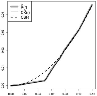
Figure 2: Empirical $K$-function (thick grey line) for the point pattern data in Figure 1(b), compensator of the $K$-function (solid black line) for a model of the correct form, and expected $K$-function for a homogeneous Poisson process (dashed line).

In special cases this diagnostic is a residual version of one of the classical functional summary statistics $K$, $G$ or $F$ obtained by subtracting a “compensator” from the functional summary statistic. The compensator depends on the fitted model, and may also depend on the observed data. For example, suppose the fitted model is the homogeneous Poisson process. Then (ignoring some details) the compensator of the empirical $K$-function $\hat{K}(r)$ is its expectation $K_{0}(r)=\pi r^{2}$ under the model, while the compensator of the empirical nearest neighbor function $\hat{G}(r)$ is the empirical empty space function $\hat{F}(r)$ for the same data. This approach provides a new class of residual summary statistics that can be used as informal diagnostics for model fit, for a wide range of point process models, in close analogy with current practice. The diagnostics apply under very general conditions, including the case of inhomogeneous point process models, where exploratory methods are underdeveloped or inapplicable. For instance, Figure 2 shows the compensator of $K(r)$ for an inhomogeneous Strauss process.

Section 2 introduces basic definitions and assumptions. Section 3 describes the score test for a general point process model, and Section 4 develops the important case of Poisson point process models. Section 5 gives examples and technical tools for non-Poisson point process models. Section 6 develops the general theory for our diagnostic tools. Section 7 applies these tools to tests for first order trend and hotspots. Sections 8–11 develop diagnostics for interaction between points, based on pairwise distances, nearest neighbor distances and empty space distances, respectively. The tools are demonstrated on data in Sections 12–15. Further examples of diagnostics are given in Appendix A. Appendices B–E provide technical details.

2 Assumptions

2.1 Fundamentals

A spatial point pattern data set is a finite set $\mathbf{x}=\{x_{1},\ldots,x_{n}\}$ of points $x_{i}\in W$, where the number of points $n(\mathbf{x})=n\geq 0$ is not fixed in advance, and the domain of observation $W\subset\mathbb{R}^{d}$ is a fixed, known region of $d$-dimensional space with finite positive volume $|W|$. We take $d=2$, but the results generalize easily to all dimensions.

A point process model assumes that $\mathbf{x}$ is a realization of a finite point process $\mathbf{X}$ in $W$ without multiple points. We can equivalently view $\mathbf{X}$ as a random finite subset of $W$. Much of the literature on spatial statistics assumes that $\mathbf{X}$ is the restriction $\mathbf{X}=\mathbf{Y}\cap W$ of a stationary point process $\mathbf{Y}$ on the entire space $\mathbb{R}^{2}$. We do not assume this; there is no assumption of stationarity, and some of the models considered here are intrinsically confined to the domain $W$. For further background material including measure theoretical details, see, for example, mollwaag04 , Appendix B.

Write $\mathbf{X}\sim\operatorname{Poisson}({W},{\rho})$ if $\mathbf{X}$ follows the Poisson process on $W$ with intensity function $\rho$, where we assume $\nu=\int_{W}\rho(u)\,\mathrm{d}u$ is finite. Then $n(\mathbf{X})$ is Poisson distributed with mean $\nu$, and, conditional on $n(\mathbf{X})$, the points in $\mathbf{X}$ are i.i.d. with density $\rho(u)/\nu$.

Every point process model considered here is assumed to have a probability density with respect to $\operatorname{Poisson}({W},{1})$, the unit rate Poisson process, under one of the following scenarios.

2.2 Unconditional Case

In the unconditional case we assume $\mathbf{X}$ has a density $f$ with respect to $\operatorname{Poisson}({W},{1})$. Then the density is characterized by the property

$$\mathbb{E}[h(\mathbf{X})]=\mathbb{E}[h(\mathbf{Y})f(\mathbf{Y})]$$ (1)

for all nonnegative measurable functionals $h$, where $\mathbf{Y}\sim\operatorname{Poisson}({W},{1})$. In particular, the density of$\operatorname{Poisson}({W},{\rho})$ is

$$f(\mathbf{x})=\exp\biggl{(}\int_{W}\bigl{(}1-\rho(u)\bigr{)}\,\mathrm{d}{u}\biggr{)}\prod_{i}\rho(x_{i}).$$ (2)

We assume that $f$ is hereditary, that is, $f(\mathbf{x})>0$ implies $f(\mathbf{y})>0$ for all finite $\mathbf{y}\subset\mathbf{x}\subset W$. Processes satisfying these assumptions include (under integrability conditions) inhomogeneous Poisson processes with an intensity function, finite Gibbs processes contained in $W$, and Cox processes driven by random fields. See illietal08 , Chapter 3, for an overview of finite point processes including these examples. In practice, our methods require the density to have a tractable form, and are only developed for Poisson and Gibbs processes.

2.3 Conditional Case

In the conditional case, we assume $\mathbf{X}=\mathbf{Y}\cap W$ where $\mathbf{Y}$ is a point process. Thus, $\mathbf{X}$ may depend on unobserved points of $\mathbf{Y}$ lying outside $W$. The density of $\mathbf{X}$ may be unknown or intractable. Under suitable conditions (explained in Section 5.4) modeling and inference can be based on the conditional distribution of ${\mathbf{X}}^{\circ}=\mathbf{X}\cap{W}^{\circ}$ given ${\mathbf{X}}^{+}=\mathbf{X}\cap{W}^{+}={\mathbf{x}}^{+}$, where ${W}^{+}\subset W$ is a subregion, typically a region near the boundary of $W$, and only the points in ${W}^{\circ}=W\setminus{W}^{+}$ are treated as random. We assume that the conditional distribution of ${\mathbf{X}}^{\circ}=\mathbf{X}\cap{W}^{\circ}$ given ${\mathbf{X}}^{+}=\mathbf{X}\cap{W}^{+}={\mathbf{x}}^{+}$ has an hereditary density $f({\mathbf{x}}^{\circ}|{\mathbf{x}}^{+})$ with respect to $\operatorname{Poisson}({{W}^{\circ}},{1})$. Processes satisfying these assumptions include Markov point processes lies00 , mollwaag04 , Section 6.4, together with all processes covered by the unconditional case. Our methods are only developed for Poisson and Markov point processes.

For ease of exposition, we focus mainly on the unconditional case, with occasional comments on the conditional case. For Poisson point process models, we always take $W={W}^{\circ}$ so that the two cases agree.

3 Score Test for Point Processes

In principle, any technique for likelihood-based inference is applicable to point process likelihoods. In practice, many likelihood computations require extensive Monte Carlo simulation geye99 , mollwaag04 , mollwaag07 . To minimize such difficulties, when assessing the goodness of fit of a fitted point process model, it is natural to choose the score test which only requires computations for the null hypothesis wald41 , rao48 .

Consider any parametric family of point process models for $\mathbf{X}$ with density $f_{\theta}$ indexed by a $k$-dimensional vector parameter $\theta\in\Theta\subseteq\mathbb{R}^{k}$. For a simple null hypothesis $H_{0}\dvtx\theta=\theta_{0}$ where $\theta_{0}\in\Theta$ is fixed, the score test against any alternative $H_{1}\dvtx\theta\in\Theta_{1}$, where $\Theta_{1}\subseteq\Theta\setminus\{\theta_{0}\}$, is based on the score test statistic (coxhink74 , page 315),

$$T^{2}={U(\theta_{0})}^{\top}I(\theta_{0})^{-1}U(\theta_{0}).$$ (3)

Here $U(\theta)=\frac{\partial}{\partial\theta}\log f_{\theta}(\mathbf{x})$ and $I(\theta)=\mathbb{E}_{\theta}[U(\theta){U(\theta)}^{\top}]$ are the score function and Fisher information, respectively, and the expectation is with respect to $f_{\theta}$. Here and throughout, we assume that the order of integration and differentation with respect to $\theta$ can be interchanged. Under suitable conditions, the null distribution of $T^{2}$ is $\chi^{2}$ with $k$ degrees of freedom. In the case $k=1$ it may be informative to evaluate the signed square root

$$T={U(\theta_{0})}/{\sqrt{I(\theta_{0})}},$$ (4)

which is asymptotically $N(0,1)$ distributed under the same conditions.

For a composite null hypothesis $H_{0}\dvtx\theta\in\Theta_{0}$ where $\Theta_{0}\subset\Theta$ is an $m$-dimensional submanifold with $0<m<k$, the score test statistic is defined in coxhink74 , page 324. However, we shall not use this version of the score test, as it assumes differentiability of the likelihood with respect to nuisance parameters, which is not necessarily applicable here (as exemplified in Section 4.2).

In the sequel we often consider models of the form

$$f_{(\alpha,\beta)}(\mathbf{x})=c(\alpha,\beta)h_{\alpha}(\mathbf{x})\exp(\beta S(\mathbf{x})),$$ (5)

where the parameter $\beta$ and the statistic $S(\mathbf{x})$ are one dimensional, and the null hypothesis is $H_{0}\dvtx\beta=0$. For fixed $\alpha$, this is a linear exponential family and (4) becomes

$$T(\alpha)=\bigl{(}S(\mathbf{x})-\mathbb{E}_{(\alpha,0)}[S(\mathbf{X})]\bigr{)}/\sqrt{\mathbb{V}\mathrm{ar}_{(\alpha,0)}[S(\mathbf{X})]}.$$

In practice, when $\alpha$ is unknown, we replace $\alpha$ by its MLE under $H_{0}$ so that, with a slight abuse of notation, the signed square root of the score test statistic is approximated by

$$\hskip 10.0ptT = T(\hat{\alpha})$$

$$= \bigl{(}S(\mathbf{x})-\mathbb{E}_{(\hat{\alpha},0)}[S(\mathbf{X})]\bigr{)}/\sqrt{\mathbb{V}\mathrm{ar}_{(\hat{\alpha},0)}[S(\mathbf{X})]}.$$

Under suitable conditions, $T$ in (3) is asymptotically equivalent to $T$ in (4), and so a standard Normal approximation may still apply.

4 Score Test for Poisson Processes

Application of the score test to Poisson point process models appears to originate with Cox cox72pp . Consider a parametric family of Poisson processes,$\operatorname{Poisson}({W},{\rho_{\theta}})$, where the intensity function is indexed by $\theta\in\Theta$. The score test statistic is (3), where

$$U(\theta) = \sum_{i}\kappa_{\theta}(x_{i})-\int_{W}\kappa_{\theta}(u)\rho_{\theta}(u)\,\mathrm{d}{u},$$

$$I(\theta) = \int_{W}{\kappa_{\theta}(u)}\,{\kappa_{\theta}(u)}^{\top}\rho_{\theta}(u)\,\mathrm{d}{u}$$

with $\kappa_{\theta}(u)=\frac{\partial}{\partial\theta}\log\rho_{\theta}(u).$ Asymptotic results are given in kuto98 , rathcres94b .

4.1 Log-Linear Alternative

The score test is commonly used in spatial epidemiology to assess whether disease incidence depends on environmental exposure. As a particular case of (5), suppose the Poisson model has a log-linear intensity function

$$\rho_{(\alpha,\beta)}(u)=\exp\bigl{(}\alpha+\beta Z(u)\bigr{)},$$ (7)

where $Z(u),u\in W$, is a known, real-valued and nonconstant covariate function, and $\alpha$ and $\beta$ are real parameters. Cox cox72pp noted that the uniformly most powerful test of $H_{0}\dvtx\beta=0$ (the homogeneous Poisson process) against $H_{1}\dvtx\beta>0$ is based on the statistic

$$S(\mathbf{x})=\sum_{i}Z(x_{i}).$$ (8)

Recall that, for a point process $\mathbf{X}$ on $W$ with intensity function $\rho$, we have Campbell’s Formula (dalevere03 , page 163),

$$\mathbb{E}\biggl{(}\sum_{x_{i}\in\mathbf{X}}h(x_{i})\biggr{)}=\int_{W}h(u)\rho(u)\,\mathrm{d}{u}$$ (9)

for any Borel function $h$ such that the integral on the right-hand side exists; and for the Poisson process $\operatorname{Poisson}({W},{\rho})$,

$$\mathbb{V}\mathrm{ar}\biggl{(}\sum_{x_{i}\in\mathbf{X}}h(x_{i})\biggr{)}=\int_{W}h(u)^{2}\rho(u)\,\mathrm{d}{u}$$ (10)

for any Borel function $h$ such that the integral on the right-hand side exists. Hence, the standardized version of (8) is

$$\hskip 20.0ptT=\biggl{(}S(\mathbf{x})-\hat{\kappa}\int_{W}Z(u)\,\mathrm{d}u\biggr{)}\Big{/}\sqrt{\hat{\kappa}\int_{W}Z(u)^{2}\,\mathrm{d}u},$$ (11)

where $\hat{\kappa}=n/|W|$ is the MLE of the intensity $\kappa=\exp(\alpha)$ under the null hypothesis. This is a direct application of the approximation (3) of the signed square root of the score test statistic.

Berman berm86 proposed several tests and diagnostics for spatial association between a point process $\mathbf{X}$ and a covariate function $Z(u)$. Berman’s $Z_{1}$ test is equivalent to the Cox score test described above. Waller et al. walletal92 and Lawson laws93a proposed tests for the dependence of disease incidence on environmental exposure, based on data giving point locations of disease cases. These are also applications of the score test. Berman conditioned on the number of points when making inference. This is in accordance with the observation that the statistic $n(\mathbf{x})$ is S-ancillary for $\beta$, while $S(\mathbf{x})$ is S-sufficient for $\beta$.

4.2 Threshold Alternative and Nuisance Parameters

Consider the Poisson process with an intensity function of “threshold” form,

$$\rho_{z,\kappa,\phi}(u)=\cases{\kappa\exp(\phi)&if $Z(u)\leq z$,\cr\kappa&if $Z(u)>z$,}$$

where $z$ is the threshold level. If $z$ is fixed, this model is a special case of (7) with $Z(u)$ replaced by ${\mathbb{I}}\{{Z(u)\leq z}\}$, and so (8) is replaced by

$$S(\mathbf{x})=S(\mathbf{x},z)=\sum_{i}{\mathbb{I}}\{{Z(x_{i})\leq z}\},$$

where ${\mathbb{I}}\{{\cdot}\}$ denotes the indicator function. By (11) the (approximate) score test of $H_{0}\dvtx\phi=0$ against $H_{1}\dvtx\phi\neq 0$ is based on

$$T=T(z)=\bigl{(}{S(\mathbf{x},z)-\hat{\kappa}A(z)}\bigr{)}/{\sqrt{\hat{\kappa}A(z)}},$$

where $A(z)=|\{u\in W\dvtx Z(u)\leq z\}|$ is the area of the corresponding level set of $Z$.

If $z$ is not fixed, then it plays the role of a nuisance parameter in the score test: the value of $z$ affects inference about the canonical parameter $\phi$, which is the parameter of primary interest in the score test. Note that the likelihood is not differentiable with respect to $z$.

In most applications of the score test, a nuisance parameter would be replaced by its MLE under the null hypothesis. However, in this context, $z$ is not identifiable under the null hypothesis. Several solutions have been proposed conn01 , davi77 , davi87 , hans96 , silv96 . They include replacing $z$ by its MLE under the alternative conn01 , maximizing $T(z)$ or $|T(z)|$ over $z$ davi77 , davi87 , and finding the maximum $p$-value of $T(z)$ or $|T(z)|$ over a confidence region for $z$ under the alternative silv96 .

These approaches appear to be inapplicable to the current context. While the null distribution of $T(z)$ is asymptotically $N(0,1)$ for each fixed $z$ as $\kappa\to\infty$, this convergence is not uniform in $z$. The null distribution of $S(\mathbf{x},z)$ is Poisson with parameter $\kappa A(z)$; sample paths of $T(z)$ will be governed by Poisson behavior where $A(z)$ is small.

In this paper, our approach is simply to plot the score test statistic as a function of the nuisance parameter. This turns the score test into a graphical exploratory tool, following the approach adopted in many other areas atki82 , cookweis83 , preg82 , chen83 , wang85 . A second style of plot based on $S(x,z)-\hat{\kappa}A(z)$ against $z$ may be more appropriate visually. Such a plot is the lurking variable plot of baddetal05 . Berman berm86 also proposed a plot of $S(\mathbf{x},z)$ against $z$, together with a plot of $\hat{\kappa}A(z)$ against $z$, as a diagnostic for dependence on $Z$. This is related to the Kolmogorov–Smirnov test since, under $H_{0}$, the values $Y_{i}=Z(x_{i})$ are i.i.d. with distribution function $\mathbb{P}(Y\leq y)=A(y)/|W|.$

4.3 Hot Spot Alternative

Consider the Poisson process with intensity

$$\rho_{\kappa,\phi,v}(u)=\kappa\exp\bigl{(}\phi k(u-v)\bigr{)},$$ (12)

where $k$ is a kernel (a probability density on $\mathbb{R}^{2}$), $\kappa>0$ and $\phi$ are real parameters, and $v\in\mathbb{R}^{2}$ is a nuisance parameter. This process has a “hot spot” of elevated intensity in the vicinity of the location $v$. By (11) and (9)–(10) the score test of $H_{0}\dvtx\phi=0$ against $H_{1}\dvtx\phi\neq 0$ is based on

$$T=T(v)=\bigl{(}S(\mathbf{x},v)-\hat{\kappa}M_{1}(v)\bigr{)}/\sqrt{\hat{\kappa}M_{2}(v)},$$

where

$$S(\mathbf{x},v)=\sum_{i}k(x_{i}-v)$$

is the usual nonparametric kernel estimate of point process intensity digg85 evaluated at $v$ without edge correction, and

$$M_{i}(v)=\int_{W}k(u-v)^{i}\,\mathrm{d}{u},\quad i=1,2.$$

The numerator $S(\mathbf{x},v)-\hat{\kappa}M_{1}(v)$ is the smoothed residual field baddetal05 of the null model. In the special case where $k(u)\propto{\mathbb{I}}\{{\|u\|\leq h}\}$ is the uniform density on a disc of radius $h$, the maximum $\max_{v}T(v)$ is closely related to the scan statistic alm88 , kull99 .

5 Non-Poisson Models

The remainder of the paper deals with the case where the alternative (and perhaps also the null) is not a Poisson process. Key examples are stated in Section 5.1. Non-Poisson models require additional tools including the Papangelou conditional intensity (Section 5.2) and pseudo-likelihood (Section 5.3).

5.1 Point Process Models with Interaction

We shall frequently consider densities of the form

$$f(\mathbf{x})=c\biggl{[}\prod_{i}\lambda(x_{i})\biggr{]}\exp(\phi V(\mathbf{x})),$$ (13)

where $c$ is a normalizing constant, the first order term $\lambda$ is a nonnegative function, $\phi$ is a real interaction parameter, and $V(\mathbf{x})$ is a real nonadditive function which specifies the interaction between the points. We refer to $V$ as the interaction potential. In general, apart from the Poisson density (2) corresponding to the case $\phi=0$, the normalizing constant is not expressible in closed form.

Often the definition of $V$ can be extended to all finite point patterns in $\mathbb{R}^{2}$ so as to be invariant under rigid motions (translations and rotations). Then the model for $\mathbf{X}$ is said to be homogeneous if $\lambda$ is constant on $W$, and inhomogeneous otherwise.

Let

$$d(u,\mathbf{x})=\min_{j}\|u-x_{j}\|$$

denote the distance from a location $u$ to its nearest neighbor in the point configuration $\mathbf{x}$. For $n(\mathbf{x})=n\geq 1$ and $i=1,\ldots,n$, define

$$\mathbf{x}_{-{i}}=\mathbf{x}\setminus\{x_{i}\}.$$

In many places in this paper we consider the following three motion-invariant interaction potentials $V(\mathbf{x})=V(\mathbf{x},r)$ depending on a parameter $r>0$which specifies the range of interaction. The Strauss process stra75 has interaction potential

$$V_{S}(\mathbf{x},r)=\sum_{i<j}{\mathbb{I}}\{{\|x_{i}-x_{j}\|\leq r}\},$$ (14)

the number of $r$-close pairs of points in $\mathbf{x}$; the Geyer saturation model geye99 with saturation threshold 1 has interaction potential

$$V_{G}(\mathbf{x},r)=\sum_{i}{\mathbb{I}}\{{d(x_{i},\mathbf{x}_{-{i}})\leq r}\},$$ (15)

the number of points in $\mathbf{x}$ whose nearest neighbor is closer than $r$ units; and the Widom–Rowlinson penetrable sphere model widorowl70 or area-interaction process baddlies95a has interaction potential

$$V_{A}(\mathbf{x},r)=-\biggl{|}W\cap\bigcup_{i}B(x_{i},r)\biggr{|},$$ (16)

the negative area of $W$ intersected with the union of balls $B(x_{i},r)$ of radius $r$ centered at the points of $\mathbf{x}$. Each of these densities favors spatial clustering (positive association) when $\phi>0$ and spatial inhibition (negative association) when $\phi<0$. The Geyer and area-interaction models are well-defined point processes for any value of $\phi$ baddlies95a , geye99 , but the Strauss density is integrable only when $\phi\leq 0$ kellripl76 .

5.2 Conditional Intensity

Consider a parametric model for a point process $\mathbf{X}$ in $\mathbb{R}^{2}$, with parameter $\theta\in\Theta$. Papangelou papa74b defined the conditional intensity of $\mathbf{X}$ as a nonnegative stochastic process $\lambda_{\theta}(u,\mathbf{X})$ indexed by locations $u\in\mathbb{R}^{2}$ and characterized by the property that

$$\mathbb{E}_{\theta}\biggl{[}\sum_{x_{i}\in\mathbf{X}}h(x_{i},\mathbf{X}\setminus\{x_{i}\})\biggr{]}$$

$$\quad=\mathbb{E}_{\theta}\biggl{[}\int_{\mathbb{R}^{2}}h(u,\mathbf{X})\lambda_{\theta}(u,\mathbf{X})\,\mathrm{d}{u}\biggr{]}$$

for all measurable functions $h$ such that the left or right-hand side exists. Equation (5.2) is known as the Georgii–Nguyen–Zessin (GNZ) formula [geor76 , kall78 , kall84 , nguyzess79a ]; see also Section 6.4.1 in mollwaag04 . Adapting a term from stochastic process theory, we will call the random integral on the right-hand side of (5.2) the (Papangelou) compensator of the random sum on the left-hand side.

Consider a finite point process $\mathbf{X}$ in $W$. In the unconditional case (Section 2.2) we assume $\mathbf{X}$ has density $f_{\theta}(\mathbf{x})$ which is hereditary for all $\theta\in\Theta$. We may simply define

$$\lambda_{\theta}(u,\mathbf{x})=f_{\theta}({\mathbf{x}}\cup\{{u}\})/f_{\theta}(\mathbf{x})$$ (18)

for all locations $u\in W$ and point configurations $\mathbf{x}\subset W$ such that $u\notin\mathbf{x}$. Here we take $0/0=0$. For $x_{i}\in\mathbf{x}$ we set $\lambda_{\theta}(x_{i},\mathbf{x})=\lambda_{\theta}(x_{i},\mathbf{x}_{-{i}})$, and for $u\notin W$ we set $\lambda_{\theta}(u,\mathbf{x})=0$. Then it may be verified directly from (1) that (5.2) holds, so that (18) is the Papangelou conditional intensity of $\mathbf{X}$. Note that the normalizing constant of $f_{\theta}$ cancels in (18). For a Poisson process, it follows from (2) and (18) that the Papangelou conditional intensity is equivalent to the intensity function of the process.

In the conditional case (Section 2.3) we assume that the conditional distribution of ${\mathbf{X}}^{\circ}=\mathbf{X}\cap{W}^{\circ}$ given ${\mathbf{X}}^{+}=\mathbf{X}\cap{W}^{+}={\mathbf{x}}^{+}$ has a hereditary density $f_{\theta}({\mathbf{x}}^{\circ}|{\mathbf{x}}^{+})$ with respect to $\operatorname{Poisson}({{W}^{\circ}},{1})$, for all $\theta\in\Theta$. Then define

$$\lambda_{\theta}(u,{\mathbf{x}}^{\circ}|{\mathbf{x}}^{+})=\frac{f_{\theta}({{\mathbf{x}}^{\circ}}\cup\{{u}\}|{\mathbf{x}}^{+})}{f_{\theta}({{\mathbf{x}}^{\circ}}\setminus\{{u}\}|{\mathbf{x}}^{+})}$$ (19)

if $u\in{W}^{\circ}$, and zero otherwise. It can similarly be verified that this is the Papangelou conditional intensity of the conditional distribution of ${\mathbf{X}}^{\circ}$ given ${\mathbf{X}}^{+}={\mathbf{x}}^{+}$.

It is convenient to rewrite (18) in the form

$$\lambda_{\theta}(u,\mathbf{x})=\exp(\Delta_{u}\log f(\mathbf{x})),$$

where $\Delta$ is the one-point difference operator

$$\Delta_{u}h(\mathbf{x})=h({\mathbf{x}}\cup\{{u}\})-h({\mathbf{x}}\setminus\{{u}\}).$$ (20)

Note the Poincaré inequality for the Poisson process $\mathbf{X}$,

$$\mathbb{V}\mathrm{ar}[h(\mathbf{X})]\leq\mathbb{E}\int_{W}[\Delta_{u}h(\mathbf{X})]^{2}\rho(u)\,\mathrm{d}{u}$$ (21)

holding for all measurable functionals $h$ such that the right-hand side is finite; see lastpenr11 , wu00 .

5.3 Pseudo-Likelihood and Pseudo-Score

To avoid computational problems with point process likelihoods, Besag besa78 introduced the pseudo-likelihood function

$$\mathsf{PL}(\theta) = \biggl{[}\prod_{i}\lambda_{\theta}(x_{i},\mathbf{x})\biggr{]}$$

$${}\cdot\exp\biggl{(}-\int_{W}\lambda_{\theta}(u,\mathbf{x})\,\mathrm{d}{u}\biggr{)}.$$

This is of the same functional form as the likelihood function of a Poisson process (2), but has the Papangelou conditional intensity in place of the Poisson intensity. The corresponding pseudo-score

$$\hskip 22.0pt\mathsf{PU}(\theta) = \frac{\partial}{\partial\theta}\log\mathsf{PL}(\theta)$$

$$= \sum_{i}\frac{\partial}{\partial\theta}\log\lambda_{\theta}(x_{i},\mathbf{x})-\int_{W}\frac{\partial}{\partial\theta}\lambda_{\theta}(u,\mathbf{x})\,\mathrm{d}{u}$$

is an unbiased estimating function, $\mathbb{E}_{\theta}\mathsf{PU}(\theta)=0$, by virtue of (5.2). In practice, the pseudo-likelihood is applicable only if the Papangelou conditional intensity $\lambda_{\theta}(u,\mathbf{x})$ is tractable.

The pseudo-likelihood function can also be defined in the conditional case jensmoll91 . In (5.3) the product is instead over points $x_{i}\in{\mathbf{x}}^{\circ}$ and the integral is instead over ${W}^{\circ}$; in (5.3) the sum is instead over points $x_{i}\in{\mathbf{x}}^{\circ}$ and the integral is instead over ${W}^{\circ}$; and in both places $\mathbf{x}={\mathbf{x}}^{\circ}\cup{\mathbf{x}}^{+}$. The Papangelou conditional intensity $\lambda_{\theta}(u,\mathbf{x})$ must also be replaced by $\lambda_{\theta}(u,{\mathbf{x}}^{\circ}|{\mathbf{x}}^{+})$.

5.4 Markov Point Processes

For a point process $\mathbf{X}$ constructed as $\mathbf{X}=\mathbf{Y}\cap W$ where $\mathbf{Y}$ is a point process in $\mathbb{R}^{2}$, the density and Papangelou conditional intensity of $\mathbf{X}$ may not be available in simple form. Progress can be made if $\mathbf{Y}$ is a Markov point process of interaction range $R<\infty$; see geor76 , nguyzess79a , riplkell77 , lies00 and mollwaag04 , Section 6.4.1. Briefly, this means that the Papangelou conditional intensity $\lambda_{\theta}(u,\mathbf{Y})$ of $\mathbf{Y}$ satisfies $\lambda_{\theta}(u,\mathbf{Y})=\lambda_{\theta}(u,\mathbf{Y}\cap\break B(u,R))$, where $B(u,R)$ is the ball of radius $R$ centered at $u$. Define the erosion of $W$ by distance $R$,

$$W_{\ominus R}=\{u\in W\dvtx B(u,R)\subset W\},$$

and assume this has nonzero area. Let $B=W\setminus W_{\ominus R}$ be the border region. The process satisfies a spatial Markov property: the processes $\mathbf{Y}\cap W_{\ominus R}$ and $\mathbf{Y}\cap W^{c}$ are conditionally independent given $\mathbf{Y}\cap B$.

In this situation we shall invoke the conditional case with ${W}^{\circ}=W_{\ominus R}$ and ${W}^{+}=W\setminus{W}^{\circ}$. The conditional distribution of $\mathbf{X}\cap{W}^{\circ}$ given $\mathbf{X}\cap{W}^{+}={\mathbf{x}}^{+}$ has Papangelou conditional intensity

$$\lambda_{\theta}(u,{\mathbf{x}}^{\circ}|{\mathbf{x}}^{+})=\cases{\lambda_{\theta}(u,{\mathbf{x}}^{\circ}\cup{\mathbf{x}}^{+})&if $u\in{W}^{\circ}$,\cr 0&otherwise.}$$ (24)

Thus, the unconditional and conditional versions of a Markov point process have the same Papangelou conditional intensity at locations in ${W}^{\circ}$.

For ${\mathbf{x}}^{\circ}=\{x_{1},\ldots,x_{{n}^{\circ}}\}$, the conditional probability density given ${\mathbf{x}}^{+}$ becomes

$$f_{\theta}({\mathbf{x}}^{\circ}|{\mathbf{x}}^{+})$$

$$\quad=c_{\theta}({\mathbf{x}}^{+})\lambda_{\theta}(x_{1},{\mathbf{x}}^{\circ})\prod_{i=2}^{{n}^{\circ}}\lambda_{\theta}(x_{i},\{x_{1},\ldots,x_{i-1}\}\cup{\mathbf{x}}^{+})$$

if ${n}^{\circ}>0$, and $f_{\theta}(\varnothing|{\mathbf{x}}^{+})=c_{\theta}({\mathbf{x}}^{+})$, where $\varnothing$ denotes the empty configuration, and the inverse normalizing constant $c_{\theta}({\mathbf{x}}^{+})$ depends only on ${\mathbf{x}}^{+}$.

For example, instead of (13) we now consider

$$f({\mathbf{x}}^{\circ}|{\mathbf{x}}^{+})=c({\mathbf{x}}^{+})\Biggl{[}\prod_{i=1}^{{n}^{\circ}}\lambda(x_{i})\Biggr{]}\exp\bigl{(}\phi V({\mathbf{x}}^{\circ}\cup{\mathbf{x}}^{+})\bigr{)},$$

assuming $V(\mathbf{y})$ is defined for all finite $\mathbf{y}\subset\mathbb{R}^{2}$ such that for any $u\in\mathbb{R}^{2}\setminus\mathbf{y}$, $\Delta_{u}V(\mathbf{y})$ depends only on $u$ and $\mathbf{y}\cap B(u,R)$. This condition is satisfied by the interaction potentials (14)–(16); note that the range of interaction is $R=r$ for the Strauss process, and $R=2r$ for both the Geyer and the area-interaction models.

6 Score, Pseudo-Score and Residual Diagnostics

This section develops the general theory for our diagnostic tools.

By (3) in Section 3 it is clear that comparison of a summary statistic $S(\mathbf{x})$ to its predicted value $\mathbb{E}S(\mathbf{X})$ under a null model is effectively equivalent to the score test under an exponential family model where $S(\mathbf{x})$ is the canonical sufficient statistic. Similarly, the use of a functional summary statistic $S(\mathbf{x},z)$, depending on a function argument $z$, is related to the score test under an exponential family model where $z$ is a nuisance parameter and $S(\mathbf{x},z)$ is the canonical sufficient statistic for fixed $z$. In this section we construct the corresponding exponential family models, apply the score test, and propose surrogates for the score test statistic.

6.1 Models

Let $f_{\theta}(\mathbf{x})$ be the density of any point process $\mathbf{X}$ on $W$ governed by a parameter $\theta$. Let $S(\mathbf{x},z)$ be a functional summary statistic of the point pattern data set $\mathbf{x}$, with function argument $z$ belonging to any space.

Consider the extended model with density

$$f_{\theta,\phi,z}(\mathbf{x})=c_{\theta,\phi,z}f_{\theta}(\mathbf{x})\exp(\phi S(\mathbf{x},z)),$$ (25)

where $\phi$ is a real parameter, and $c_{\theta,\phi,z}$ is the normalizing constant. The density is well-defined provided

$$M(\theta,\phi,z)=\mathbb{E}[f_{\theta}(\mathbf{Y})\exp(\phi S(\mathbf{Y},z))]<\infty,$$

where $\mathbf{Y}\sim\operatorname{Poisson}({W},{1})$. The extended model is constructed by “exponential tilting” of the original model by the statistic $S$. By (3), for fixed $\theta$ and $z$, assuming differentiability of $M$ with respect to $\phi$ in a neighborhood of $\phi=0$, the signed root of the score test statistic is approximated by

$$T=\bigl{(}{S(\mathbf{x},z)-\mathbb{E}_{\hat{\theta}}[S(\mathbf{X},z)]}\bigr{)}/\sqrt{\mathbb{V}\mathrm{ar}_{\hat{\theta}}[S(\mathbf{X},z)]},$$ (26)

where $\hat{\theta}$ is the MLE under the null model, and the expectation and variance are with respect to the null model with density $f_{\hat{\theta}}$.

Insight into the qualitative behavior of the extended model (25) can be obtained by studying the perturbing model

$$g_{\phi,z}(\mathbf{x})=k_{\phi,z}\exp(\phi S(\mathbf{x},z)),$$ (27)

provided this is a well-defined density with respect to $\operatorname{Poisson}({W},{1})$, where $k_{\phi,z}$ is the normalizing constant. When the null hypothesis is a homogeneous Poisson process, the extended model is identical to the perturbing model, up to a change in the first order term. In general, the extended model is a qualitative hybrid between the null and perturbing models.

In this context the score test is equivalent to naive comparison of the observed and null-expected values of the functional summary statistic $S$. The test statistic $T$ in (26) may be difficult to evaluate; typically, apart from Poisson models, the moments (particularly the variance) of $S$ would not be available in closed form. The null distribution of $T$ would also typically be unknown. Hence, implementation of the score test would typically require moment approximation and simulation from the null model, which in both cases may be computationally expensive. Various approximations for the score or the score test statistic can be constructed, as discussed in the sequel.

6.2 Pseudo-Score of Extended Model

The extended model (25) is an exponential family with respect to $\phi$, having Papangelou conditional intensity

$$\kappa_{\theta,\phi,z}(u,\mathbf{x})=\lambda_{\theta}(u,\mathbf{x})\exp(\phi\Delta_{u}S(\mathbf{x},z)),$$

where $\lambda_{\theta}(u,\mathbf{x})$ is the Papangelou conditional intensity of the null model. The pseudo-score function with respect to $\phi$, evaluated at $\phi=0$, is

$$\mathsf{PU}(\theta,z)=\sum_{i}\Delta_{x_{i}}S(\mathbf{x},z)-\int_{W}\Delta_{u}S(\mathbf{x},z)\lambda_{\theta}(u,\mathbf{x})\,\mathrm{d}{u},$$

where the first term

$$\Sigma\Delta S(\mathbf{x},z)=\sum_{i}\Delta_{x_{i}}S(\mathbf{x},z)$$ (28)

will be called the pseudo-sum of $S$. If $\hat{\theta}$ is the maximum pseudo-likelihood estimate (MPLE) under $H_{0}$, the second term with $\theta$ replaced by $\hat{\theta}$ becomes

$$\mathcal{C}\Delta S(\mathbf{x},z)=\int_{W}\Delta_{u}S(\mathbf{x},z)\lambda_{\hat{\theta}}(u,\mathbf{x})\,\mathrm{d}{u}$$ (29)

and will be called the (estimated) pseudo-compensator of $S$. We call

$$\mathcal{R}\Delta S(\mathbf{x},z) = \mathsf{PU}(\hat{\theta},z)$$

$$= \Sigma\Delta S(\mathbf{x},z)-\mathcal{C}\Delta S(\mathbf{x},z)$$

the pseudo-residual since it is a weighted residual in the sense of baddetal05 .

The pseudo-residual serves as a surrogate for the numerator in the score test statistic (26). For the denominator, we need the variance of the pseudo-residual. Appendix B gives an exact formula (B.2) for the variance of the pseudo-score $\mathsf{PU}(\theta,z)$, which can serve as an approximation to the variance of the pseudo-residual $\mathcal{R}\Delta S(\mathbf{x},z)$. This is likely to be an overestimate, because the effect of parameter estimation is typically to deflate the residual variance baddetal05 .

The first term in the variance formula (B.2) is

$$\mathcal{C}^{2}\Delta S(\mathbf{x},z)=\int_{W}[\Delta_{u}S(\mathbf{x},z)]^{2}\lambda_{\hat{\theta}}(u,\mathbf{x})\,\mathrm{d}{u},$$ (31)

which we shall call the Poincaré pseudo-variance because of its similarity to the Poincaré upper bound in (21). It is easy to compute this quantity alongside the pseudo-residual. Rough calculations in Sections 9.4 and 10.3 suggest that the Poincaré pseudo-variance is likely to be the dominant term in the variance, except at small $r$ values. The variance of residuals is also studied in coeulava10 .

For computational efficiency we propose to use the square root of (31) as a surrogate for the denominator in (26). This yields a “standardized” pseudo-residual

$$\qquad\mathcal{T}\Delta S(\mathbf{x},z)=\mathcal{R}\Delta S(\mathbf{x},z)/\sqrt{\mathcal{C}^{2}\Delta S(\mathbf{x},z)}.$$ (32)

We emphasize that this quantity is not guaranteed to have zero mean and unit variance (even approximately) under the null hypothesis. It is merely a computationally efficient surrogate for the score test statistic; its null distribution must be investigated by other means. Asymptotics of $\mathcal{T}\Delta S(\mathbf{x},z)$ undera large-domain limit stei95 could be studied, but limit results are unlikely to hold uniformly over $r$. In this paper we evaluate null distributions using Monte Carlo methods.

The pseudo-sum (28) can be regarded as a functional summary statistic for the data in its own right. Its definition depends only on the choice of the statistic $S$, and it may have a meaningful interpretation as a nonparametric estimator of a property of the point process. The pseudo-compensator (29) might also be regarded as a functional summary statistic, but its definition involves the null model. If the null model is true, we may expect the pseudo-residual to be approximately zero. Sections 9–11 and Appendix A study particular instances of pseudo-residual diagnostics based on (28)–(6.2).

In the conditional case, the Papangelou conditional intensity $\lambda_{\hat{\theta}}(u,\mathbf{x})$ must be replaced by $\lambda_{\hat{\theta}}(u,\break{\mathbf{x}}^{\circ}|{\mathbf{x}}^{+})$ given in (19) or (24). The integral in the definition of the pseudo-compensator (29) must be restricted to the domain ${W}^{\circ}$, and the summation over data points in (28) must be restricted to points $x_{i}\in{W}^{\circ}$, that is, to summation over points of ${\mathbf{x}}^{\circ}$.

6.3 Residuals

A simpler surrogate for the score test is available when the canonical sufficient statistic $S$ of the perturbing model is naturally expressible as a sum of local contributions

$$S(\mathbf{x},z)=\sum_{i}s(x_{i},\mathbf{x}_{-{i}},z).$$ (33)

Note that any statistic can be decomposed in this way unless some restriction is imposed on $s$; such a decomposition is not necessarily unique. We call the decomposition “natural” if $s(u,\mathbf{x},z)$ only depends on points of $\mathbf{x}$ that are close to $u$, as demonstrated in the examples in Sections 9, 10 and 11 and in Appendix A.

Consider a null model with Papangelou conditional intensity $\lambda_{\theta}(u,\mathbf{x})$. Following baddetal05 , define the ($s$-weighted) innovation by

$$\hskip 25.0pt\mathcal{I}S(\mathbf{x},r)=S(\mathbf{x},z)-\int_{W}s(u,\mathbf{x},z)\lambda_{\theta}(u,\mathbf{x})\,\mathrm{d}{u},$$ (34)

which by the GNZ formula (5.2) has mean zero under the null model. In practice, we replace $\theta$ by an estimate $\hat{\theta}$ (e.g., the MPLE) and consider the ($s$-weighted) residual

$$\mathcal{R}S(\mathbf{x},z)=S(\mathbf{x},z)-\int_{W}s(u,\mathbf{x},z)\lambda_{\hat{\theta}}(u,\mathbf{x})\,\mathrm{d}{u}.$$ (35)

The residual shares many properties of the score function and can serve as a computationally efficient surrogate for the score. The data-dependent integral

$$\mathcal{C}S(\mathbf{x},z)=\int_{W}s(u,\mathbf{x},z)\lambda_{\hat{\theta}}(u,\mathbf{x})\,\mathrm{d}{u}$$ (36)

is the (estimated) Papangelou compensator of $S$. The variance of $\mathcal{R}S(\mathbf{x},z)$ can be approximated by the innovation variance, given by the general variance formula (B.1) of Appendix B. The first term in (B.1) is the Poincaré variance

$$\mathcal{C}^{2}S(\mathbf{x},z)=\int_{W}s(u,\mathbf{x},z)^{2}\lambda_{\hat{\theta}}(u,\mathbf{x})\,\mathrm{d}{u}.$$ (37)

Rough calculations reported in Sections 9.4 and 10.3 suggest that the Poincaré variance is likely to be the largest term in the variance for sufficiently large $r$. By analogy with (31) we propose to use the Poincaré variance as a surrogate for the variance of $\mathcal{R}S(\mathbf{x},z)$, and thereby obtain a “standardized” residual

$$\mathcal{T}S(\mathbf{x},z)=\mathcal{R}S(\mathbf{x},z)/\sqrt{\mathcal{C}^{2}S(\mathbf{x},z)}.$$ (38)

Once again $\mathcal{T}S(\mathbf{x},z)$ is not exactly standardized, because $\mathcal{C}^{2}S(\mathbf{x},z)$ is an approximation to $\mathbb{V}\mathrm{ar}[\mathcal{R}S(\mathbf{x},z)]$ and because the numerator and denominator of (38) are dependent. The null distribution of $\mathcal{T}S(\mathbf{x},z)$must be investigated by other means.

In the conditional case, the integral in the definition of the compensator (36) must be restricted to the domain ${W}^{\circ}$, and the summation over data points in (33) must be restricted to points $x_{i}\in{W}^{\circ}$, that is, to summation over points of ${\mathbf{x}}^{\circ}$.

7 Diagnostics for First Order Trend

Consider any null model with density $f_{\theta}(\mathbf{x})$ and Papangelou conditional intensity $\lambda_{\theta}(u,\mathbf{x})$. By analogy with Section 4 we consider alternatives of the form (25) where

$$S(\mathbf{x},z)=\sum_{i}s(x_{i},z)$$

for some function $s$. The perturbing model (27) is a Poisson process with intensity $\exp(\phi s(\cdot,z))$,where $z$ is a nuisance parameter. The score test is a test for the presence of an (extra) first order trend. The pseudo-score and residual diagnostics are both equal to

$$\mathcal{R}S(\mathbf{x},z) = \sum_{i}s(x_{i},z)$$

$${}-\int_{W}s(u,z)\lambda_{\hat{\theta}}(u,\mathbf{x})\,\mathrm{d}{u}.$$

This is the $s$-weighted residual described in baddetal05 . The variance of (7) can be estimated by simulation, or approximated by the Poincaré variance (37).

If $Z$ is a real-valued covariate function on $W$, then we may take $s(u,z)={\mathbb{I}}\{{Z(u)\leq z}\}$ for $z\in\mathbb{R}$, corresponding to a threshold effect (cf. Section 4.2). A plot of (7) against $z$ was called a lurking variable plot in baddetal05 .

If $s(u,z)=k(u-z)$ for $z\in\mathbb{R}^{2}$, where $k$ is a density function on $\mathbb{R}^{2}$, then

$$\mathcal{R}S(\mathbf{x},z)=\sum_{i}k(x_{i}-z)-\int_{W}k(u-z)\lambda_{\hat{\theta}}(u,\mathbf{x})\,\mathrm{d}{u},$$

which was dubbed the smoothed residual field in baddetal05 . Examples of application of these techniques have been discussed extensively in baddetal05 .

8 Interpoint Interaction

In the remainder of the paper we concentrate on diagnostics for interpoint interaction.

8.1 Classical Summary Statistics

Following Ripley’s influential paper ripl77 , it is standard practice, when investigating association or dependence between points in a spatial point pattern, to evaluate functional summary statistics such as the $K$-function, and to compare graphically the empirical summaries and theoretical predicted values under a suitable model, often a stationary Poisson process (“Complete Spatial Randomness,” CSR) ripl77 , cres91 , digg03 .

The three most popular functional summary statistics for spatial point processes are Ripley’s $K$-function, the nearest neighbor distance distribution function $G$ and the empty space function (spherical contact distance distribution function) $F$. Definitions of $K$, $G$ and $F$ and their estimators can be seen in badd99b , cres91 , digg03 , mollwaag04 . Simple empirical estimators of these functions are of the form

$$\hat{K}(r) = \hat{K}_{\mathbf{x}}(r)$$

$$= \frac{1}{\hat{\rho}{}^{2}(\mathbf{x})|W|}\sum_{i\neq j}e_{K}(x_{i},x_{j}){\mathbb{I}}\{{\|x_{i}-x_{j}\|\leq r}\},$$

$$\hat{G}(r) = \hat{G}_{\mathbf{x}}(r)$$

$$= \frac{1}{n(\mathbf{x})}\sum_{i}e_{G}(x_{i},\mathbf{x}_{-{i}},r){\mathbb{I}}\{{d(x_{i},\mathbf{x}_{-{i}})\leq r}\},$$

$$\hat{F}(r) = \hat{F}_{\mathbf{x}}(r)$$

$$= \frac{1}{|W|}\int_{W}e_{F}(u,r){\mathbb{I}}\{{d(u,\mathbf{x})\leq r}\}\,\mathrm{d}{u},$$

where $e_{K}(u,v)$, $e_{G}(u,\mathbf{x},r)$ and $e_{F}(u,r)$ are edge correction weights, and typically $\hat{\rho}{}^{2}(\mathbf{x})=n(\mathbf{x})(n(\mathbf{x})-1)/|W|^{2}$.

8.2 Score Test Approach

The classical approach fits naturally into thescheme of Section 6. In order to test for dependence between points, we choose a perturbing model that exhibits dependence. Three interesting examples of perturbing models are the Strauss process, the Geyer saturation model with saturation threshold 1 and the area-interaction process, with interaction potentials $V_{S}(\mathbf{x},r)$, $V_{G}(\mathbf{x},r)$ and $V_{A}(\mathbf{x},r)$ given in (14)–(16). The nuisance parameter $r\geq 0$ determines the range of interaction. It is interesting to note that, although the Strauss density is integrable only when $\phi\leq 0$, the extended model obtained by perturbing $f_{\theta}$ by the Strauss density may be well-defined for some $\phi>0$. This extended model may support alternatives that are clustered relative to the null, as originally intended by Strauss stra75 .

The potentials of these three models are closely related to the summary statistics $\hat{K},\hat{G}$ and $\hat{F}$ in (8.1)–(8.1). Ignoring the edge correction weights $e(\cdot)$, we have

$$\hat{K}_{\mathbf{x}}(r) \approx \frac{2|W|}{n(\mathbf{x})(n(\mathbf{x})-1)}V_{S}(\mathbf{x},r),$$ (43)

$$\hat{G}_{\mathbf{x}}(r) \approx \frac{1}{n(\mathbf{x})}V_{G}(\mathbf{x},r),$$ (44)

$$\hat{F}_{\mathbf{x}}(r) \approx -\frac{1}{|W|}V_{A}(\mathbf{x},r).$$ (45)

To draw the closest possible connection with the score test, instead of choosing the Strauss, Geyer or area-interaction process as the perturbing model, we shall take the perturbing model to be defined through (27) where $S$ is one of the statistics $\hat{K}$, $\hat{G}$ or $\hat{F}$. We call these the (perturbing) $\hat{K}$-model, $\hat{G}$-model and $\hat{F}$-model, respectively. The score test is then precisely equivalent to comparing $\hat{K}$, $\hat{G}$ or $\hat{F}$ with its predicted expectation using (3).

Essentially $\hat{K}$, $\hat{G}$, $\hat{F}$ are renormalized versionsof $V_{S}$, $V_{G}$, $V_{A}$ as shown in (43)–(45). In the case of $\hat{F}$ the renormalization is not data-dependent, so the $\hat{F}$-model is virtually an area-interaction model, ignoring edge correction. For $\hat{K}$, the renormalization depends only on $n(\mathbf{x})$, and so, conditionally on $n(\mathbf{x})=n$, the $\hat{K}$-model and the Strauss process are approximately equivalent. Similarly for $\hat{G}$, the normalization also depends only on $n(\mathbf{x})$, so, conditionally on $n(\mathbf{x})=n$, the $\hat{G}$-model and Geyer saturation process are approximately equivalent. If we follow Ripley’s ripl77 recommendation to condition on $n$ when testing for interaction, this implies that the use of the $K$, $G$ or $F$-function is approximately equivalent to the score test of CSR against a Strauss, Geyer or area-interaction alternative, respectively.

When the null hypothesis is CSR, we saw that the extended model (25) is identical to the perturbing model, up to a change in intensity, so that the use of the $\hat{K}$-function is equivalent to testing the null hypothesis of CSR against the alternative of a $\hat{K}$-model; similarly for $\hat{G}$ and $\hat{F}$. For a more general null hypothesis, the use of the $\hat{K}$-function, for example, corresponds to adopting an alternative hypothesis that is a hybrid between the fitted model and a $\hat{K}$-model.

Note that if the edge correction weight $e_{K}(u,v)$ is uniformly bounded, the $\hat{K}$-model is integrable for all values of $\phi$, avoiding a difficulty with the Strauss process kellripl76 .

Computation of the score test statistic (26) requires estimation or approximation of the null variance of $\hat{K}(r)$, $\hat{G}(r)$ or $\hat{F}(r)$. A wide variety of approximations is available when the null hypothesis is CSR ripl88 , digg03 . For other null hypotheses, simulation estimates would typically be used. A central limit theorem is available for $\hat{K}(r)$, $\hat{G}(r)$ and $\hat{F}(r)$ in the large-domain limit, for example, badd80b , hein88 , hein88b , joli80 , ripl88 . However, convergence is not uniform in $r$, and the normal approximation will be poor for small values of $r$. Instead Ripley ripl76 developed an exact Monte Carlo test barn63 , hope68 based on simulation envelopes of the summary statistic under the null hypothesis.

In the following sections we develop the residual and pseudo-residual diagnostics corresponding to this approach.

9 Residual Diagnostics for Interaction Using Pairwise Distances

This section develops residual (35) and pseudo-residual (6.2) diagnostics derived from a summary statistic $S$ which is a sum of contributions depending on pairwise distances.

9.1 Residual Based on Perturbing Strauss Model

9.1.1 General derivation

Consider any statistic of the general “pairwise interaction” form

$$S(\mathbf{x},r)=\sum_{i<j}q(\{x_{i},x_{j}\},r).$$ (46)

This can be decomposed in the local form (33) with

$$s(u,\mathbf{x},r)=\frac{1}{2}\sum_{i}q(\{x_{i},u\},r),\quad u\notin\mathbf{x}.$$

Hence,

$$\Delta_{x_{i}}S(\mathbf{x},r) = 2s(x_{i},\mathbf{x}_{-{i}},r)\quad\mbox{and}$$

$$\Delta_{u}S(\mathbf{x},r) = 2s(u,\mathbf{x},r),\quad u\notin\mathbf{x}.$$

Consequently, the pseudo-residual and the pseudo-compensator are just twice the residual and the Papangelou compensator:

$$\hskip 30.0pt\Sigma\Delta S(\mathbf{x},r) = 2S(\mathbf{x},r)=\sum_{i\neq j}q(\{x_{i},x_{j}\},r),$$ (47)

$$\hskip 30.0pt\mathcal{C}\Delta S(\mathbf{x},r) = 2\mathcal{C}S(\mathbf{x},r)$$

$$= \int_{W}\sum_{i}q(\{x_{i},u\},r)\lambda_{\hat{\theta}}(u,\mathbf{x})\,\mathrm{d}{u},$$

$$\hskip 30.0pt\mathcal{R}\Delta S(\mathbf{x},z) = 2\mathcal{R}S(\mathbf{x},r)$$

$$= 2S(\mathbf{x},r)-2\mathcal{C}S(\mathbf{x},r).$$

9.1.2 Residual of Strauss potential

The Strauss interaction potential $V_{S}$ of (14) is of the generalform (46) with $q(\{x_{i},x_{j}\},r)={\mathbb{I}}\{{\|x_{i}-x_{j}\|\leq r}\}$.Hence, $V_{S}$ can be decomposed in the form (33) with $s(u,\mathbf{x},r)=\frac{1}{2}t(u,\mathbf{x},r)$, where

$$t(u,\mathbf{x},r)=\sum_{i}{\mathbb{I}}\{{\|u-x_{i}\|\leq r}\},\quad u\notin\mathbf{x}.$$

Hence, the Papangelou compensator of $V_{S}$ is

$$\mathcal{C}V_{S}(\mathbf{x},r)=\frac{1}{2}\int_{W}t(u,\mathbf{x},r)\lambda_{\hat{\theta}}(u,\mathbf{x})\,\mathrm{d}{u}.$$ (50)

9.1.3 Case of CSR

If the null model is CSR with intensity $\rho$ estimated by $\hat{\rho}=n(\mathbf{x})/|W|$ (the MLE, which agrees with the MPLE in this case), the Papangelou compensator (50) becomes

$$\mathcal{C}V_{S}(\mathbf{x},r) = \frac{\hat{\rho}}{2}\int_{W}\sum_{i}{\mathbb{I}}\{{\|u-x_{i}\|\leq r}\}\,\mathrm{d}{u}$$

$$= \frac{\hat{\rho}}{2}\sum_{i}|W\cap B(x_{i},r)|.$$

Ignoring edge effects, we have $|W\cap B(x_{i},r)|\approx\pi r^{2}$ and, applying (43), the residual is approximately

$$\mathcal{R}V_{S}(\mathbf{x},r)\approx\frac{n(\mathbf{x})^{2}}{2|W|}[\hat{K}_{\mathbf{x}}(r)-\pi r^{2}].$$ (51)

The term in brackets is a commonly-used measure of departure from CSR, and is a sensible diagnostic because $K(r)=\pi r^{2}$ under CSR.

9.2 Residual Based on Perturbing $\hat{K}$-Model

Assuming $\hat{\rho}^{2}(\mathbf{x})=\hat{\rho}^{2}(n(\mathbf{x}))$ depends only on $n(\mathbf{x})$, the empirical $K$-function (8.1) can also be expressed as a sum of local contributions $\hat{K}_{\mathbf{x}}(r)=\sum_{i}k(x_{i},\break\mathbf{x}_{-{i}},r)$ with

$$k(u,\mathbf{x},r)=\frac{t^{w}(u,\mathbf{x},r)}{\hat{\rho}^{2}(n(\mathbf{x})+1)|W|},\quad u\notin\mathbf{x},$$

where

$$t^{w}(u,\mathbf{x},r)=\sum_{j}e_{K}(u,x_{j}){\mathbb{I}}\{{\|u-x_{j}\|\leq r}\}$$

is a weighted count of the points of $\mathbf{x}$ that are $r$-close to the location $u$. Hence, the compensator of the $\hat{K}$-function is

$$\mathcal{C}\hat{K}_{\mathbf{x}}(r) = \frac{1}{\hat{\rho}^{2}(n(\mathbf{x})+1)|W|}$$

$${}\cdot\int_{W}t^{w}(u,\mathbf{x},r)\lambda_{\hat{\theta}}(u,\mathbf{x})\,\mathrm{d}{u}.$$

Assume the edge correction weight $e_{K}(u,v)=\break e_{K}(v,u)$ is symmetric; for example, this is satisfied by the Ohser–Stoyan edge correction weight ohsestoy81 , ohse83 given by $e_{K}(u,v)=1/|W_{u}\cap W_{v}|$ where $W_{u}=\{u+v\dvtx\break v\in W\}$, but not by Ripley’s ripl76 isotropic correction weight. Then the increment is, for $u\notin\mathbf{x}$,

$$\Delta_{u}\hat{K}_{\mathbf{x}}(r) = \frac{\hat{\rho}^{2}(\mathbf{x})-\hat{\rho}^{2}({\mathbf{x}}\cup\{{u}\})}{\hat{\rho}^{2}({\mathbf{x}}\cup\{{u}\})}\hat{K}_{\mathbf{x}}(r)$$

$${}+\frac{2t^{w}(u,\mathbf{x},r)}{\hat{\rho}^{2}({\mathbf{x}}\cup\{{u}\})|W|}$$

and when $x_{i}\in\mathbf{x}$

$$\Delta_{x_{i}}\hat{K}_{\mathbf{x}}(r) = \frac{\hat{\rho}^{2}(\mathbf{x}_{-{i}})-\hat{\rho}^{2}(\mathbf{x})}{\hat{\rho}^{2}(\mathbf{x}_{-{i}})}\hat{K}_{\mathbf{x}}(r)$$

$${}+\frac{2t^{w}(x_{i},\mathbf{x}_{-i},r)}{\hat{\rho}^{2}(\mathbf{x}_{-{i}})|W|}.$$

Assuming the standard estimator $\hat{\rho}^{2}(\mathbf{x})=n(n-1)/\break|W|^{2}$ with $n=n(\mathbf{x})$, the pseudo-sum is seen to be zero, so the pseudo-residual is apart from the sign equal to the pseudo-compensator, which becomes

$$\mathcal{C}\Delta\hat{K}_{\mathbf{x}}(r)=2\mathcal{C}\hat{K}_{\mathbf{x}}(r)-\biggl{[}\frac{2}{n-2}\int_{W}\lambda_{\hat{\theta}}(u,\mathbf{x})\,\mathrm{d}u\biggr{]}\hat{K}_{\mathbf{x}}(r),$$

where $\mathcal{C}\hat{K}_{\mathbf{x}}(r)$ is given by (9.2). So if the null model is CSR and the intensity is estimated by $n/|W|$, the pseudo-residual is approximately $2[\hat{K}_{\mathbf{x}}(r)-\mathcal{C}\hat{K}_{\mathbf{x}}(r)]$, and, hence, it is equivalent to the residual approximated by (51). This is also the conclusion in the more general case of a null model with an activity parameter $\kappa$, that is, where the Papangelou conditional intensity factorizes as

$$\lambda_{\theta}(u,\mathbf{x})=\kappa\xi_{\beta}(u,\mathbf{x}),$$

where $\theta=(\kappa,\beta)$ and $\xi_{\beta}(\cdot)$ is a Papangelou conditional intensity, since the pseudo-likelihood equations then imply that $n=\int_{W}\lambda_{\hat{\theta}}(u,\mathbf{x})\,\mathrm{d}u$.

In conclusion, the residual diagnostics obtained from the perturbing Strauss and $\hat{K}$-models are very similar, the major difference being the data-dependent normalization of the $\hat{K}$-function; similarly for pseudo-residual diagnostics which may be effectively equivalent to the residual diagnostics. In practice, the popularity of the $K$-function seems to justify using the residual diagnostics based on the perturbing $\hat{K}$-model. Furthermore, due to the familiarity of the $K$-function, we often choose to plot the compensator(s) of the fitted model(s) in a plot with the empirical $K$-function rather than the residual(s) for the fitted model.

9.3 Edge Correction in Conditional Case

In the conditional case, the Papangelou conditional intensity $\lambda_{\hat{\theta}}(u,\mathbf{x})$ is known only at locations $u\in{W}^{\circ}$. The diagnostics must be modified accordingly, by restricting the domain of summation and integration to ${W}^{\circ}$. Appropriate modifications are discussed in Appendices C–E.

9.4 Approximate Residual Variance Under CSR

Here we study the residual variance and the accuracy of the Poincaré variance approximation in a simple case.

We shall approximate the residual variance$\mathbb{V}\mathrm{ar}[\mathcal{R}V_{S}(X,r)]$ by the innovation variance$\mathbb{V}\mathrm{ar}[\mathcal{I}V_{S}(X,r)]$, that is, ignoring the effect of parameter estimation. It is likely that this approximation is conservative, because the effect of parameter estimation is typically to deflate the residual variance baddetal05 . A more detailed investigation has been conducted in coeulava10 .

Assume the null model is CSR with intensity $\rho$ estimated by $\hat{\rho}=n(\mathbf{x})/|W|$. The exact variance of the innovation for the Strauss canonical statistic $V_{S}$ is $\mathbb{V}\mathrm{ar}[\mathcal{I}V_{S}(\mathbf{X},r)]=I_{1}+I_{2}$ from equation (B.1) of Appendix B, where

$$I_{1} = \frac{1}{4}\int_{W}\mathbb{E}[t(u,\mathbf{X},r)^{2}\lambda(u,\mathbf{X})]\,\mathrm{d}{u}$$

$$= \frac{\rho}{4}\int_{W}\mathbb{E}[t(u,\mathbf{X},r)^{2}]\,\mathrm{d}{u}$$

and

$$I_{2} = \frac{1}{4}\int_{W}\int_{W}\mathbb{E}[{\mathbb{I}}\{{\|u-v\|\leq r}\}\lambda_{2}(u,v,\mathbf{X})]\,\mathrm{d}{u}\,\mathrm{d}{v}$$

$$= \frac{\rho^{2}}{4}\int_{W}\int_{W}{\mathbb{I}}\{{\|u-v\|\leq r}\}\,\mathrm{d}{u}\,\mathrm{d}{v}$$

as $\lambda(u,\mathbf{X})=\rho$ and $\lambda_{2}(u,v,\mathbf{X})=\lambda(u,\mathbf{X})\lambda(v,\break\mathbf{X}\cup\{u\})=\rho^{2}$. This is reminiscent of expressions for the large-domain limiting variance of $\hat{K}$ under CSR obtained using the methods of $U$-statistics lotwsilv82 , chetdigg98 , ripl88 , summarized in digg03 , page 51 ff. Now $Y=t(u,\mathbf{X},r)$ is Poisson distributed with mean $\mu=\break\rho|B(u,r)\cap W|$ so that $\mathbb{E}(Y^{2})=\mu+\mu^{2}$. For $u\in W_{\ominus r}$ we have $\mu=\rho\pi r^{2}$, so ignoring edge effects

$$I_{1}\approx\frac{\rho}{4}(\nu+\nu^{2})|W|\quad\mbox{and}\quad I_{2}\approx\frac{\rho}{4}\nu|W|,$$

where $\nu=\rho\pi r^{2}$. Note that since $\nu$ is the expected number of points within distance $r$ of a given point, a value of $\nu=1$ corresponds to the scale of nearest-neighbor distances in the pattern, $r_{\mathrm{nn}}=1/\sqrt{\pi\rho}.$ For the purposes of the $K$ function this is a “short” distance. Hence, it is reasonable to describe $I_{1}$ as the “leading term” in the variance, since $I_{1}\gg I_{2}$ for $\nu\gg 1$.

Meanwhile, the Poincaré variance (37) is

$$\mathcal{C}^{2}V_{S}(\mathbf{x},r)=\frac{n(\mathbf{x})}{4|W|}\int_{W}t(u,\mathbf{x},r)^{2}\,\mathrm{d}{u},$$

which is an approximately unbiased estimator of $I_{1}$ by Fubini’s Theorem. Hence,

$$\frac{\mathbb{E}\mathcal{C}^{2}V_{S}(\mathbf{x},r)}{\mathbb{V}\mathrm{ar}[\mathcal{R}V_{S}(\mathbf{X},r)]} \approx \frac{\mathbb{E}\mathcal{C}^{2}V_{S}(\mathbf{x},r)}{\mathbb{V}\mathrm{ar}[\mathcal{I}V_{S}(\mathbf{X},r)]}$$

$$\approx \frac{I_{1}}{I_{1}+I_{2}}\approx\frac{1+\nu}{2+\nu}.$$

Thus, as a rule of thumb, the Poincaré variance underestimates the true variance; the ratio of means is $(1+\nu)/(2+\nu)\geq 1/2$. The ratio falls to $2/3$ when $\nu=1$, that is, when $r=r_{\mathrm{nn}}=1/\sqrt{\pi\rho}$. We can take this as a rule-of-thumb indicating the value of $r$ below which the Poincare variance is a poor approximation to the true variance.

10 Residual Diagnostics for Interaction Using Nearest Neighbor Distances

This section develops residual and pseudo-residual diagnostics derived from summary statistics based on nearest neighbor distances.

10.1 Residual Based on Perturbing Geyer Model

The Geyer interaction potential $V_{G}(\mathbf{x},r)$ givenby (15) is clearly a sum of local statistics (33), and its compensator is

$$\mathcal{C}V_{G}(\mathbf{x},r)=\int_{W}{\mathbb{I}}\{{d(u,\mathbf{x})\leq r}\}\lambda_{\hat{\theta}}(u,\mathbf{x})\,\mathrm{d}{u}.$$

The Poincaré variance is equal to the compensator in this case. Ignoring edge effects, $V_{G}(\mathbf{x},r)$ is approximately $n(\mathbf{x})\hat{G}_{\mathbf{x}}(r)$; cf. (8.1).

If the null model is CSR with estimated intensity $\hat{\kappa}=n(\mathbf{x})/|W|$, then

$$\mathcal{C}V_{G}(\mathbf{x},r)=\hat{\kappa}\biggl{|}W\cap\bigcup_{i}B(x_{i},r)\biggr{|};$$

ignoring edge effects, this is approximately $\hat{\kappa}|W|\hat{F}(r)$; cf. (8.1). Thus, the residual diagnostic is approximately $n(\mathbf{x})(\hat{G}(r)-\hat{F}(r))$. This is a reasonable diagnostic for departure from CSR, since $F\equiv G$ under CSR. This argument lends support to Diggle’s digg79a , equation (5.7), proposal to judge departure from CSR using the quantity $\sup|\hat{G}-\hat{F}|$.

This example illustrates the important point that the compensator of a functional summary statistic $S$ should not be regarded as an alternative parametric estimator of the same quantity that $S$ is intended to estimate. In the example just given, under CSR the compensator of $\hat{G}$ is approximately $\hat{F}$, a qualitatively different and in some sense “opposite” summary of the point pattern.

We have observed that the interaction potential $V_{G}$ of the Geyer saturation model is closely related to $\hat{G}$. However, the pseudo-residual associated to $V_{G}$ is a more complicated statistic, since a straightforward calculation shows that the pseudo-sum is

$$\Sigma\Delta V_{G}(\mathbf{x},r)$$

$$\quad=V_{G}(\mathbf{x},r)+\sum_{i}\sum_{j:j\not=i}\mathbb{I}\{\|x_{i}-x_{j}\|\leq r\mbox{ and}$$

$$\hskip 136.0ptd(x_{j},\mathbf{x}_{-{i}})>r\},$$

and the pseudo-compensator is

$$\mathcal{C}\Delta V_{G}(\mathbf{x},r) = \int_{W}{\mathbb{I}}\{{d(u,\mathbf{x})\leq r}\}\lambda_{\hat{\theta}}(u,\mathbf{x})\,\mathrm{d}{u}$$

$${}+\sum_{i}{\mathbb{I}}\{{d(x_{i},\mathbf{x}_{-{i}})>r}\}$$

$$\phantom{{}+\sum_{i}}{}\cdot\int_{W}{\mathbb{I}}\{{\|u-x_{i}\|\leq r}\}\lambda_{\hat{\theta}}(u,\mathbf{x})\,\mathrm{d}{u}.$$

10.2 Residual Based on Perturbing $\hat{G}$-Model

The empirical $G$-function (8.1) can be written

$$\hat{G}_{\mathbf{x}}(r)=\sum_{i}g(x_{i},\mathbf{x}_{-{i}},r),$$ (53)

where

$$g(u,\mathbf{x},r) = \frac{1}{n(\mathbf{x})+1}e_{G}(u,\mathbf{x},r)$$

$${}\cdot{\mathbb{I}}\{{d(u,\mathbf{x})\leq r}\},\quad u\notin\mathbf{x},$$

so that the Papangelou compensator of the empirical $G$-function is

$$\mathcal{C}\hat{G}_{\mathbf{x}}(r)$$

$$\quad=\int_{W}g(u,\mathbf{x},r)\lambda_{\hat{\theta}}(u,\mathbf{x})\,\mathrm{d}{u}$$

$$\quad=\frac{1}{n(\mathbf{x})+1}\int_{W\cap\bigcup_{i}B(x_{i},r)}e_{G}(u,\mathbf{x},r)\lambda_{\hat{\theta}}(u,\mathbf{x})\,\mathrm{d}{u}.$$

The residual diagnostics obtained from the Geyer and $\hat{G}$-models are very similar, and we choose to use the diagnostic based on the popular $\hat{G}$-function. As with the $K$-function, we typically use the compensator(s) of the fitted model(s) rather than the residual(s), to visually maintain the close connection to the empirical $G$-function.

The expressions for the pseudo-sum and pseudo-compensator of $\hat{G}$ are not of simple form, and we refrain from explicitly writing out these expressions. For both the $\hat{G}$- and Geyer models, the pseudo-sum and pseudo-compensator are not directly related to a well-known summary statistic. We prefer to plot the pseudo-residual rather than the pseudo-sum and pseudo-compensator(s).

10.3 Residual Variance Under CSR

Again assume a Poisson process of intensity $\rho$ as the null model. Since $V_{G}$ is a sum of local statistics,

$$V_{G}(\mathbf{x},r)=\sum_{i}{\mathbb{I}}\{{d(x_{i},\mathbf{x}\setminus x_{i})\leq r}\},$$

we can again apply the variance formula (B.1) of Appendix B, which gives $\mathbb{V}\mathrm{ar}[\mathcal{I}V_{G}(\mathbf{X},r)]=L_{1}+L_{2},$ where

$$L_{1}=\rho\int_{W}\mathbb{P}\{d(u,\mathbf{X})\leq r\}\,\mathrm{d}{u}$$

and

$$L_{2} = \rho^{2}\int_{W}\int_{W}\mathbb{P}\{\|u-v\|\leq r,$$

$$\phantom{\rho^{2}\int_{W}\int_{W}\mathbb{P}\{}d(u,X)>r,\,d(v,X)>r\}\,\mathrm{d}{u}\,\mathrm{d}{v}.$$

The Poincaré variance is equal to the compensator in this case, and is

$$\mathcal{C}^{2}V_{G}(\mathbf{x},r) = \int_{W}{\mathbb{I}}\{{d(u,\mathbf{x})\leq r}\}\lambda_{\hat{\theta}}(u,\mathbf{x})\,\mathrm{d}{u}$$

$$= \frac{n(\mathbf{x})}{|W|}|W\cap U(\mathbf{x},r)|,$$

where $U(\mathbf{x},r)=\bigcup_{i}b(x_{i},r)$. The Poincaré variance is an approximately unbiased estimator of the term $L_{1}$.

For $u\in W_{\ominus r}$ we have $\mathbb{P}\{d(u,\mathbf{X})\leq r\}=1-\break\exp(-\rho\pi r^{2})$ so that

$$L_{1}\approx\rho|W|\bigl{(}1-\exp(-\rho\pi r^{2})\bigr{)},$$

ignoring edge effects. Again, let $\nu=\rho\pi r^{2}$ so that $L_{1}\approx\rho|W|(1-\exp(-\nu))$. Meanwhile,

$$\mathbb{P}\{d(u,X)>r,\,d(v,X)>r\}$$

$$\quad=\exp\bigl{(}-\rho|b(u,r)\cup b(v,r)|\bigr{)}.$$

This probability lies between $\exp(-\nu)$ and $\exp(-2\nu)$ for all $u,v$. Thus (ignoring edge effects),

$$L_{2} \approx \rho^{2}\pi r^{2}|W|\exp\bigl{(}-(1+\delta)\nu\bigr{)}$$

$$= \rho\nu|W|\exp\bigl{(}-(1+\delta)\nu\bigr{)},$$

where $0\leq\delta\leq 1$. Hence,

$$\frac{L_{2}}{L_{1}}\leq\frac{\nu e^{-\nu}}{1-e^{-\nu}}.$$

Let $f(\nu)=\nu e^{-\nu}/(1-e^{-\nu})$. Then $f(\nu)$ is strictly decreasing and $f(\nu)<1$ for all $\nu>0$ so that $L_{1}/\break(L_{1}+L_{2})\geq\frac{1}{2},$ that is, the variance is underestimated by at most a factor of 2. Note that $f(1.25)\approx 0.5$, so $L_{1}/(L_{1}+L_{2})\geq\frac{2}{3}$ when $r\leq r_{\mathrm{crit}}$, where $r_{\mathrm{crit}}=\sqrt{1.25/\pi\rho}.$ The conclusions and rule-of-thumb for $\mathcal{T}\hat{G}$ are similar to those obtained for $\mathcal{T}\hat{K}$ in Section 9.4.

11 Diagnostics for Interaction Based on Empty Space Distances

11.1 Pseudo-Residual Based on Perturbing Area-Interaction Model

When the perturbing model is the area-interaction process, it is convenient to reparametrize the density, such that the canonical sufficient statistic $V_{A}$ given in (16) is redefined as

$$V_{A}(\mathbf{x},r)=\frac{1}{|W|}\biggl{|}W\cap\bigcup_{i}B(x_{i},r)\biggr{|}.$$

This summary statistic is not naturally expressed as a sum of contributions from each point as in (33), so we shall only construct the pseudo-residual. Let

$$U(\mathbf{x},r)=W\cap\bigcup_{i}B(x_{i},r).$$

The increment

$$\Delta_{u}V_{A}(\mathbf{x},r)$$

$$\quad=\frac{1}{|W|}\bigl{(}|U({\mathbf{x}}\cup\{{u}\},r)|-|U(\mathbf{x},r)|\bigr{)},\quad u\notin\mathbf{x},$$

can be thought of as “unclaimed space”—the proportion of space around the location $u$ that is not “claimed” by the points of $\mathbf{x}$. The pseudo-sum

$$\Sigma\Delta V_{A}(\mathbf{x},r)=\sum_{i}\Delta_{x_{i}}V_{A}(\mathbf{x},r)$$

is the proportion of the window that has “single coverage”—the proportion of locations in $W$ that are covered by exactly one of the balls $B(x_{i},r)$. This can be used in its own right as a functional summary statistic, and it corresponds to a raw (i.e., not edge corrected) empirical estimate of a summary function $F_{1}(r)$ defined by

$$F_{1}(r)=\mathbb{P}\bigl{(}\#\{x\in\mathbf{X}|d(u,x)\leq r\}=1\bigr{)}$$

for any stationary point process $\mathbf{X}$, where $u\in\mathbb{R}^{2}$ is arbitrary. Under CSR with intensity $\rho$ we have

$$F_{1}(r)=\rho\pi r^{2}\exp(-\rho\pi r^{2}).$$

This summary statistic does not appear to be treated in the literature, and it may be of interest to study it separately, but we refrain from a more detailed study here.

The pseudo-compensator corresponding to thispseudo-sum is

$$\mathcal{C}\Delta V_{A}(\mathbf{x},r)=\int_{W}\Delta_{u}V_{A}(\mathbf{x},r)\lambda_{\hat{\theta}}(u,\mathbf{x})\,\mathrm{d}{u}.$$

This integral does not have a particularly simple interpretation even when the null model is CSR.

11.2 Pseudo-Residual Based on Perturbing $\hat{F}$-Model

Alternatively, one could use a standard empirical estimator $\hat{F}$ of the empty space function $F$ as the summary statistic in the pseudo-residual. The pseudo-sum associated with the perturbing $\hat{F}$-model is

$$\Sigma\Delta\hat{F}_{\mathbf{x}}(r)=n(\mathbf{x})\hat{F}_{\mathbf{x}}(r)-\sum_{i}\hat{F}_{\mathbf{x}_{-{i}}}(r),$$

with pseudo-compensator

$$\mathcal{C}\Delta\hat{F}_{\mathbf{x}}(r)=\int_{W}\bigl{(}\hat{F}_{{\mathbf{x}}\cup\{{u}\}}(r)-\hat{F}_{\mathbf{x}}(r)\bigr{)}\lambda_{\hat{\theta}}(u,\mathbf{x})\,\mathrm{d}{u}.$$

Ignoring edge correction weights, $\hat{F}_{{\mathbf{x}}\cup\{{u}\}}(r)-\hat{F}_{\mathbf{x}}(r)$ is approximately equal to $\Delta_{u}V_{A}(\mathbf{x},r)$, so the pseudo-sum and pseudo-compensator associated with the perturbing $\hat{F}$-model are approximately equal to the pseudo-sum and pseudo-compensator associated with the perturbing area-interaction model. Here, we usually prefer graphics using the pseudo-compensator(s) and the pseudo-sum since this has an intuitive interpretation as explained above.

12 Test Case: Trend with Inhibition

In Sections 12–14 we demonstrate the diagnostics on the point pattern data sets shown in Figure 1. This section concerns the synthetic point pattern in Figure 1(b).

12.1 Data and Models

Figure 1(b) shows a simulated realization of the inhomogeneous Strauss process with first order term $\lambda(x,y)=200\exp(2x+2y+3x^{2})$, interaction range $R=0.05$, interaction parameter $\gamma=\exp(\phi)=0.1$ and $W$ equal to the unit square; see (13) and (14). This is an example of extremely strong inhibition (negative association) between neighboring points, combined with a spatial trend. Since it is easy to recognize spatial trend in the data (either visually or using existing tools such as kernel smoothing digg85 ), the main challenge here is to detect the inhibition after accounting for the trend.

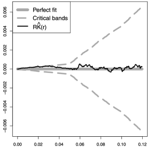
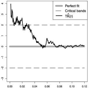
(a)	(b)

Figure 3: Residual diagnostics based on pairwise distances, for a model of the correct form fitted to the data in Figure 1(b). (a) Residual $\hat{K}$-function and two-standard-deviation limits under the fitted model of the correct form. (b) Standardized residual $\hat{K}$-function under the fitted model of the correct form.

We fitted four point process models to the data in Figure 1(b). They were (A) a homogeneous Poisson process (CSR); (B) an inhomogeneous Poisson process with the correct form of the first order term, that is, with intensity

$$\rho(x,y)=\exp(\beta_{0}+\beta_{1}x+\beta_{2}y+\beta_{3}x^{2}),$$ (55)

where $\beta_{0},\ldots,\beta_{3}$ are real parameters; (C) a homogeneous Strauss process with the correct interaction range $R=0.05$; and (D) a process of the correct form, that is, inhomogeneous Strauss with the correct interaction range $R=0.05$ and the correct form of the first order potential (55).

12.2 Software Implementation

The diagnostics defined in Sections 9–11 were implemented in the R language, and has been publicly released in the spatstat library baddturn05 . Unless otherwise stated, models were fitted by approximate maximum pseudo-likelihood using the algorithm of baddturn00 with the default quadrature scheme in spatstat, having an $m\times m$ grid of dummy points where $m=\max(25,10[1+2\sqrt{n(\mathbf{x})}/10])$ was equal to 40 for most of our examples. Integrals over the domain $W$ were approximated by finite sums over the quadrature points. Some models were refitted using a finer grid of dummy points, usually $80\times 80$. In addition to maximum pseudo-likelihood estimation, the software also supports the Huang–Ogata huanogat99 approximate maximum likelihood.

12.3 Application of $\hat{K}$ Diagnostics

12.3.1 Diagnostics for correct model

First we fitted a point process model of the correct form (D). The fitted parameter values were $\hat{\gamma}=0.217$ and $\hat{\beta}=(5.6,-0.46,3.35,2.05)$ using the coarse grid of dummy points, and $\hat{\gamma}=0.170$ and $\hat{\beta}=(5.6,-0.64,4.06,\break 2.44)$ using the finer grid of dummy points, as against the true values $\gamma=0.1$ and $\beta=(5.29,2,2,3)$.

Figure 2 in Section 1 shows $\hat{K}$ along with its compensator for the fitted model, together with the theoretical $K$-function under CSR. The empirical $K$-function and its compensator coincide very closely, suggesting correctly that the model is a good fit. Figure 3(a) shows the residual $\hat{K}$-function and the two-standard-deviation limits, where the surrogate standard deviation is the square root of (37). Figure 3(b) shows the corresponding standardized residual $\hat{K}$-function obtained by dividing by the surrogate standard deviation.

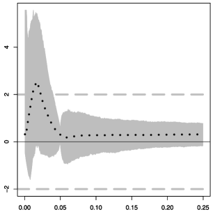
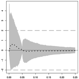
(a)	(b)

Figure 4: Null distribution of standardized residual of $\hat{K}$. Pointwise 2.5% and 97.5% quantiles (grey shading) and sample mean (dotted lines) of $\mathcal{T}\hat{K}$ from 1000 simulated realizations of model (D) with estimated parameter values (a) $\hat{\gamma}=0.217$ and $\hat{\beta}=\break(5.6,-0.46,3.35,2.05)$ using a $40\times 40$ grid of dummy points; (b) $\hat{\gamma}=0.170$ and $\hat{\beta}=(5.6,-0.64,4.06,2.44)$ using a $80\times 80$ grid.

Although this model is of the correct form, the standardized residual exceeds 2 for small values of $r$. This is consistent with the prediction in Section 9.4 that the variance approximation would be inaccurate for small $r$. The null model is a nonstationary Poisson process; the minimum value of the intensity is $200$. Taking $\rho=200$ and applying the rule of thumb in Section 9.4 gives

$$r_{\mathrm{nn}}=\frac{1}{\sqrt{200\pi}}=0.04,$$

suggesting that the Poincaré variance estimate becomes unreliable for $r\leq 0.04$ approximately.

Formal significance interpretation of the critical bands in Figure 3(b) is limited, because the null distribution of the standardized residual is not known exactly, and the values $\pm 2$ are approximate pointwise critical values, that is, critical values for the score test based on fixed $r$. The usual problems of multiple testing arise when the test statistic is considered as a function of $r$; see digg03 , page 14. For very small $r$ there are small-sample effects so that a normal approximation to the null distribution of the standardized residual is inappropriate.

To confirm this, Figure 4 shows the pointwise 2.5% and 97.5% quantiles of the null distribution of $\mathcal{T}\hat{K}$, obtained by extensive simulation. The sample mean of the simulated $\mathcal{T}\hat{K}$ is also shown, and indicates that the expected standardized residual is nonzero for small values of $r$. Repeating the computation with a finer grid of quadrature points (for approximating integrals over $W$ involved in the pseudo-likelihood and the residuals) reduces the bias, suggesting that this is a discretization artefact.

12.3.2 Comparison of competing models

Figu-re 5(a) shows the empirical $K$-function and its compensator for each of the models (A)–(D) in Section 12.1. Figure 5(b) shows the corresponding residual plots, and Figure 5(c) the standardized residuals. A positive or negative value of the residual suggests that the data are more clustered or more inhibited, respectively, than the model. The clear inference is that the Poisson models (A) and (B) fail to capture interpoint inhibition at range $r\approx 0.05$, while the homogeneous Strauss model (C) is less clustered than the data at very large scales, suggesting that it fails to capture spatial trend. The correct model (D) is judged to be a good fit.

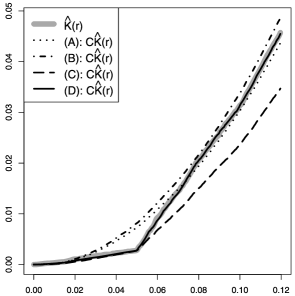
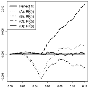
(a)	(b)
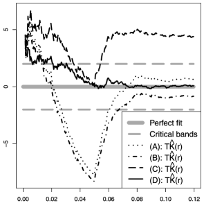
(c)

Figure 5: Model diagnostics based on pairwise distances, for each of the models (A)–(D) fitted to the data in Figure 1(b). (a) $\hat{K}$ and its compensator under each model. (b) Residual $\hat{K}$-function (empirical minus compensator) under each model. (c) Standardized residual $\hat{K}$-function under each model.

The interpretation of this example requires some caution, because the residual $\hat{K}$-function of the fitted Strauss models (C) and (D) is constrained to be approximately zero at $r=R=0.05$. The maximum pseudo-likelihood fitting algorithm solves an estimating equation that is approximately equivalent to this constraint, because of (43).

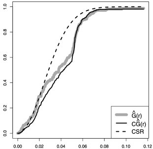
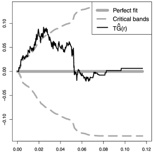
(a)	(b)

Figure 6: Residual diagnostics obtained from the perturbing $\hat{G}$-model when the data pattern is a realization of an inhomogeneous Strauss process. (a) $\hat{G}$ and its compensator under a fitted model of the correct form, and theoretical $G$-function for a Poisson process. (b) Residual $\hat{G}$-function and two-standard-deviation limits under the fitted model of the correct form.

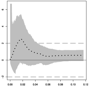
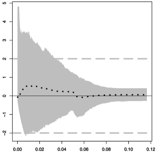
(a)	(b)

Figure 7: Null distribution of standardized residual of $\hat{G}$. Pointwise 2.5% and 97.5% quantiles (grey shading) and sample mean (dotted lines) from 1000 simulated realizations of model (D) with estimated parameter values (a) $\hat{\gamma}=0.217$ and $\hat{\beta}=(5.6,-0.46,3.35,2.05)$ using a $40\times 40$ grid of dummy points; (b) $\hat{\gamma}=0.170$ and $\hat{\beta}=(5.6,-0.64,4.06,2.44)$ using a $80\times 80$ grid.

It is debatable which of the presentations in Figure 5 is more effective at revealing lack of fit. A compensator plot such as Figure 5(a) seems best at capturing the main differences between competing models. It is particularly useful for recognizing a gross lack of fit. A residual plot such as Figure 5(b) seems better for making finer comparisons of model fit, for example, assessing models with slightly different ranges of interaction. A standardized residual plot such as Figure 5(c) tends to be highly irregular for small values of $r$, due to discretization effects in the computation and the inherent nondifferentiability of the empirical statistic. In difficult cases we may apply smoothing to the standardized residual.

12.4 Application of $\hat{G}$ Diagnostics

12.4.1 Diagnostics for correct model

Consideragain the model of the correct form (D). The residual and compensator of the empirical nearest neighbor function $\hat{G}$ for the fitted model are shown in Figure 6. The residual plot suggests a marginal lack of fit for $r<0.025$. This may be correct, since the fitted model parameters (Section 12.3.1) are marginally poor estimates of the true values, in particular, of the interaction parameter. This was not reflected so strongly in the $\hat{K}$ diagnostics. This suggests that the residual of $\hat{G}$ may be particularly sensitive to lack of fit of interaction.

Applying the rule of thumb in Section 10.3, we have $r_{\mathrm{crit}}=0.044$, agreeing with the interpretation that the $\pm 2$ limits are not trustworthy for $r<0.05$ approximately.

Figure 7 shows the pointwise 2.5% and 97.5% quantiles of the null distribution of $\mathcal{T}\hat{G}$. Again, there is a suggestion of bias for small values of $r$ which appears to be a discretization artefact.

12.4.2 Comparison of competing models

For each of the four models, Figure 8(a) shows $\hat{G}$ and its Papangelou compensator. This clearly shows that the Poisson models (A) and (B) fail to capture interpoint inhibition in the data. The Strauss models (C) and (D) appear virtually equivalent in Figure 8(a).

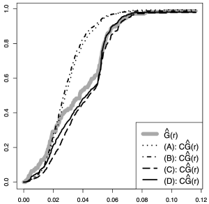
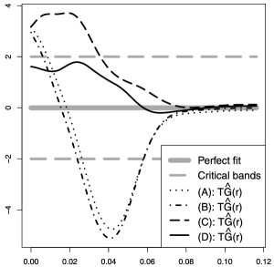
(a)	(b)
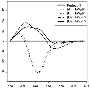
(c)

Figure 8: Diagnostics based on nearest neighbor distances, for the models (A)–(D) fitted to the data in Figure 1(b). (a) Compensator for $\hat{G}$. (b) Smoothed standardized residual of $\hat{G}$. (c) Smoothed pseudo-residual derived from a perturbing Geyer model.

Figure 8(b) shows the standardized residual of $\hat{G}$, and Figure 8(c) the pseudo-residual of $V_{G}$ (i.e., the pseudo-residual based on the pertubing Geyer model), with spline smoothing applied to both plots. The Strauss models (C) and (D) appear virtually equivalent in Figure 8(c). The standardized residual plot Figure 8(b) correctly suggests a slight lack of fit for model (C) while model (D) is judged to be a reasonable fit.

12.5 Application of $\hat{F}$ Diagnostics

Figure 9 shows the pseudo-residual diagnosticsbased on empty space distances. Both diagnostics clearly show models (A)–(B) are poor fits to data. However, in Figure 9(a) it is hard to decide whichof the models (C)–(D) provide a better fit. Despite the close connection between the area-interaction process and the $\hat{F}$-model, the diagnostic in Figu-re 9(b) based on the $\hat{F}$-model performs better in this particular example and correctly shows (D) is the best fit to data. In both cases it is noticed that the pseudo-sum has a much higher peak than the pseudo-compensators for the Poisson models (A)–(B), correctly suggesting that these models do not capture the strength of inhibition present in the data.

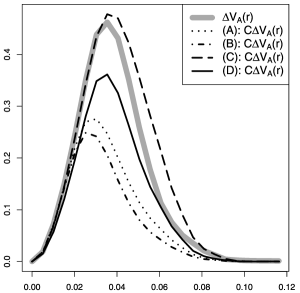
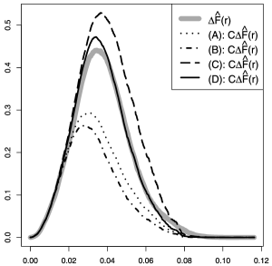
(a)	(b)

Figure 9: Pseudo-sum and pseudo-compensators for the models (A)–(D) fitted to the data in Figure 1(b) when the perturbing model is (a) the area-interaction process (null fitted on a fine grid) and (b) the $\hat{F}$-model (null fitted on a coarse grid).

13 Test Case: Clustering Without Trend

13.1 Data and Models

Figure 1(c) is a realization of a homogeneous Geyer saturation process geye99 on the unit square, with first order term $\lambda=\exp(4)$, saturation threshold $s=4.5$ and interaction parameters $r=0.05$ and $\gamma=\break\exp(0.4)\approx 1.5$, that is, the density is

$$\qquad f(\mathbf{x})\propto\exp\bigl{(}n(\mathbf{x})\log\lambda+V_{G,s}(\mathbf{x},r)\log\gamma\bigr{)},$$ (56)

where

$$V_{G,s}(\mathbf{x},r)=\sum_{i}\min\biggl{\{}s,\sum_{j:j\neq i}{\mathbb{I}}\{{\|x_{i}-x_{j}\|\leq r}\}\biggr{\}}.$$

This is an example of moderately strong clustering (with interaction range $R=2r=0.1$) without trend. The main challenge here is to correctly identify the range and type of interaction.

We fitted three point process models to the data: (E) a homogeneous Poisson process (CSR); (F) a homogeneous area-interaction process with disc radius $r=0.05$; (G) a homogeneous Geyer saturation process of the correct form, with interaction parameter $r=0.05$ and saturation threshold $s=4.5$ while the parameters $\lambda$ and $\gamma$ in (56) are unknown. The parameter estimates for (G) were $\log\hat{\lambda}=4.12$ and $\log\hat{\gamma}=0.38$.

13.2 Application of $\hat{K}$ Diagnostics

A plot (not shown) of the $\hat{K}$-function and its compensator, under each of the three models (E)–(G), demonstrates clearly that the homogeneous Poisson model (E) is a poor fit, but does not discriminate between the other models.

Figure 10 shows the residual $\hat{K}$ and the smoothed standardized residual $\hat{K}$ for the three models. These diagnostics show that the homogeneous Poisson model (E) is a poor fit, with a positive residual suggesting correctly that the data are more clustered than the Poisson process. The plots suggests that both models (F) and (G) are considerably better fits to the data than a Poisson model. They show that (G) is a better fit than (F) over a range of $r$ values, and suggest that (G) captures the correct form of the interaction.

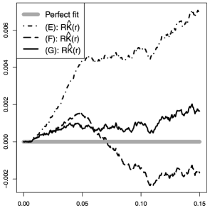
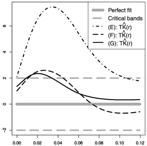
(a)	(b)

Figure 10: Model diagnostics based on pairwise distances for each of the models (E)–(G) fitted to the data in Figure 1(c). (a) Residual $\hat{K}$; (b) smoothed standardized residual $\hat{K}$.

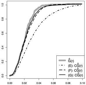
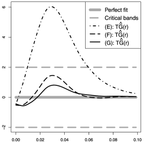
(a)	(b)

Figure 11: Model diagnostics based on nearest neighbor distances for each of the models (E)–(G) fitted to the data in Figure 1(c). (a) $\hat{G}$ and its compensator under each model; (b) smoothed standardized residual $\hat{G}$.

13.3 Application of $\hat{G}$ Diagnostics

Figure 11 shows $\hat{G}$ and its compensator, and the corresponding residuals and standardized residuals, for each of the models (E)–(G) fitted to the clustered point pattern in Figure 1(c). The conclusions obtained from Figure 11(a) are the same as those in Section 13.2 based on $\hat{K}$ and its compensator. Figure 12 shows the smoothed pseudo-residual diagnostics based on the nearest neighbor distances. The message from these diagnostics is very similar to that from Figure 11.

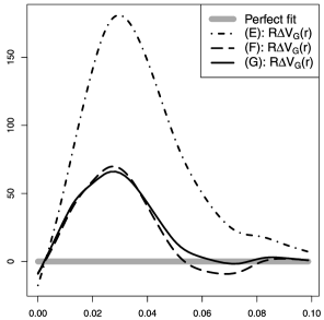
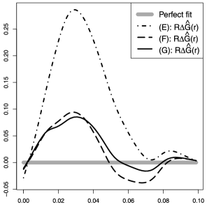
(a)	(b)

Figure 12: Smoothed pseudo-residuals for each of the models (E)–(G) fitted to the clustered point pattern in Figure 1(c) when the perturbing model is (a) the Geyer saturation model with saturation 1 and (b) the $\hat{G}$-model.

Models (F) and (G) have the same range of interaction $R=0.1$. Comparing Figures 10 and 11, we might conclude that the $\hat{G}$-compensator appears less sensitive to the form of interaction than the $\hat{K}$-compensator. Other experiments suggest that $\hat{G}$ is more sensitive than $\hat{K}$ to discrepancies in the range of interaction.

13.4 Application of $\hat{F}$ Diagnostics

Figure 13 shows the pseudo-residual diagnostics based on the empty space distances, for the three models fitted to the clustered point pattern in Figure 1(c). In this case diagnostics based on the area-interaction process and the $\hat{F}$-model are very similar, as expected due to the close connection between the two diagnostics. Here it is very noticeable that the pseudo-compensator for the Poisson model has a higher peak than the pseudo-sum, which correctly indicates that the data is more clustered than a Poisson process.

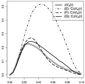
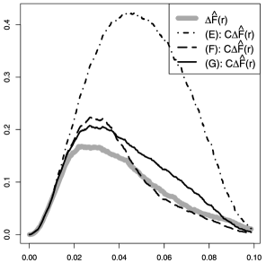
(a)	(b)

Figure 13: Pseudo-sum and pseudo-compensators for the models (E)–(G) fitted to the clustered point pattern in Figure 1(c) when the perturbing model is (a) the area-interaction process and (b) the $\hat{F}$-model.

14 Test Case: Japanese Pines

14.1 Data and Models

Figure 1(a) shows the locations of seedlings and saplings of Japanese black pine, studied by Numata numa61 , numa64 and analyzed extensively by Ogata and Tanemura ogattane81 , ogattane86 . In their definitive analysis ogattane86 the fitted model was an inhomogeneous “soft core” pairwise interaction process with log-cubic first order term $\lambda_{\beta}(x,y)=\exp(P_{\beta}(x,y))$, where $P_{\beta}$ is a cubic polynomial in $x$ and $y$ with coefficient vector $\beta$, and density

$$\hskip 15.0ptf_{(\beta,\sigma^{2})}(\mathbf{x}) = c_{(\beta,\sigma^{2})}\exp\biggl{(}\sum_{i}P_{\beta}(x_{i})$$

$$\phantom{c_{(\beta,\sigma^{2})}\exp\biggl{(}}{}-\sum_{i<j}(\sigma^{4}/\|x_{i}-x_{j}\|^{4})\biggr{)},$$

where $\sigma^{2}$ is a positive parameter.

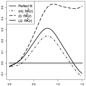
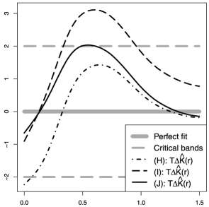
(a)	(b)

Figure 14: Model diagnostics based on pairwise distances for each of the models (H)–(J) fitted to the Japanese pines data in Figure 1(a). (a) Smoothed residual $\hat{K}$; (b) smoothed standardized residual $\hat{K}$.

Here we evaluate three models: (H) an inhomogeneous Poisson process with log-cubic intensity;(I) a homogeneous soft core pairwise interaction process, that is, when $P_{\beta}(x,y)$ in (14.1) is replaced by a real parameter; (J) the Ogata–Tanemura mo-del (14.1). For more detail on the data set and the fitted inhomogeneous soft core model, see ogattane86 , baddetal05 .

A complication in this case is that the soft core process (14.1) is not Markov, since the pair potential $c(u,v)=\exp(-\sigma^{4}/\|u-v\|^{4})$ is always positive. Nevertheless, since this function decays rapidly, it seems reasonable to apply the residual and pseudo-residual diagnostics, using a cutoff distance $R$ such that $|\log c(u,v)|\leq\varepsilon$ when $\|u-v\|\leq R$, for a specified tolerance $\varepsilon$. The cutoff depends on the fitted parameter value $\sigma^{2}$. We chose $\varepsilon=0.0002$, yielding $R=1$. Estimated interaction parameters were $\hat{\sigma}^{2}=0.11$ for model (I) and $\hat{\sigma}^{2}=0.12$ for model (J).

14.2 Application of $\hat{K}$ Diagnostics

A plot (not shown) of $\hat{K}$ and its compensator for each of the models (H)–(J) suggests that the homogeneous soft core model (I) is inadequate, while the inhomogeneous models (H) and (J) are reasonably good fits to the data. However, it does not discriminate between the models (H) and (J).

Figure 14 shows smoothed versions of the residual and standardized residual of $\hat{K}$ for each model. The Ogata–Tanemura model (J) is judged to be the best fit.

14.3 Application of $\hat{G}$ diagnostics

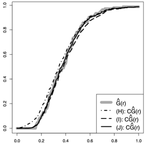
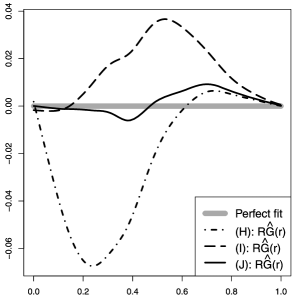
(a)	(b)
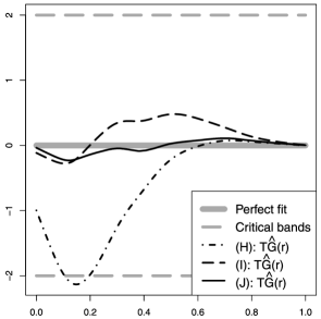
(c)

Figure 15: Model diagnostics based on nearest neighbour distances for each of the models (H)–(J) fitted to the Japanese pines data in Figure 1(a). (a) $\hat{G}$ and its compensator; (b) smoothed residual $\hat{G}$; (c) smoothed standardised residual $\hat{G}$.

Finally, for each of the models (H)–(J) fitted to the Japanese pines data in Figure 1(a), Figure 15(a) shows $\hat{G}$ and its compensator. The conclusions are the same as those based on $\hat{K}$ shown in Figure 14. Figure 16 shows the pseudo-residuals when using either a perturbing Geyer model [Figure 16(a)] or a perturbing $\hat{G}$-model [Figure 16(b)]. Figures 16(a)–(b) tell almost the same story: the inhomogeneous Poisson model (H) provides the worst fit, while it is difficult to discriminate between the fit for the soft core models (I) and (J). In conclusion, considering Figures 14, 15 and 16, the Ogata–Tanemura model (J) provides the best fit.

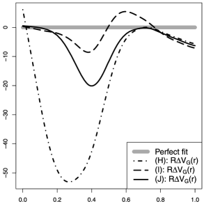
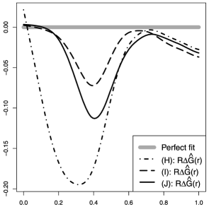
(a)	(b)

Figure 16: Smoothed pseudo-residuals for each of the models (H)–(J) fitted to the Japanese pines data in Figure 1(a) when the perturbing model is (a) the Geyer saturation model with saturation 1 (null fitted on a fine grid) and (b) the $\hat{G}$-model.

14.4 Application of $\hat{F}$ diagnostics

Finally, the empty space pseudo-residual diagnostics are shown in Figure 17 for the Japanese Pines data in Figure 1(a). This gives a clear indication that the Ogata–Tanemura model (J) is the best fit to the data, and the data pattern appears to be too regular compared to the Poisson model (H) and not regular enough for the homogeneous softcore model (I).

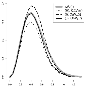
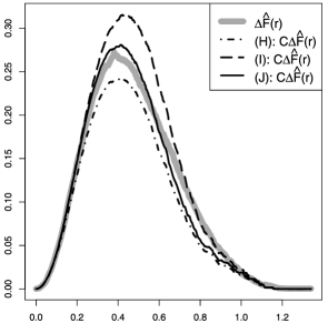
(a)	(b)

Figure 17: Pseudo-sum and pseudo-compensators for the models (H)–(J) fitted to the real data pattern in Figure 1(a) when the perturbing model is (a) the area-interaction process and (b) the $\hat{F}$-model.

15 Summary of Test Cases

In this section we discuss which of the diagnostics we prefer to use based on their behavior for the three test cases in Sections 12–14.

Typically, the various diagnostics supplement each other well, and it is recommended to use more than one diagnostic when validating a model. It is well known that $\hat{K}$ is sensitive to features at a larger scale than $\hat{G}$ and $\hat{F}$. Compensator and pseudo-compensator plots are informative for gaining an overall picture of model validity, and tend to make it easy to recognize a poor fit when comparing competing models. To compare models which fit closely, it may be more informative to use (standardized) residuals or pseudo-residuals. We prefer to use the standardized residuals, but it is important not to over-interpret the significance of departure from zero.

Based on the test cases here, it is not clear whether diagnostics based on pairwise distances, nearestneighbor distances, or empty space distances are preferable. However, for each of these we prefer to work with compensators and residuals rather than pseudo-compensators and pseudo-residuals when possible (i.e., it is only necessary to use pseudo-versions for diagnostics based on empty space distances). For instance, for the first test case (Section 12) the best compensator plot is that in Figure 5(a) based on pairwise distances ($\hat{K}$ and $\mathcal{C}\hat{K}$) which makes it easy to identify the correct model. On the other hand, in this test case the best residual type plot is that in Figure 8(b) based on nearest neighbor distances ($\mathcal{T}\hat{G}$) where the correct model is the only one within the critical bands. However, in the third test case (Section 14) the best compensator plot is one of the plots in Figure 17 with pseudo-compensators based on empty space distances ($\Sigma\Delta V_{A}$ and $\mathcal{C}\Delta V_{A}$ or $\Sigma\Delta\hat{F}$ and $\mathcal{C}\Delta\hat{F}$, respectively) which clearly indicates which model is correct.

In the first and third test cases (Sections 12and 14), which both involve inhomogeneous models, it is clear that $\hat{K}$ and its compensator are more sensitive to lack of fit in the first order term than $\hat{G}$ and its compensator [compare, e.g., the results for the homogeneous model (C) in Figures 5(a) and 8(b)]. It is our general experience that diagnostics based on $\hat{K}$ are particularly well suited to assess the presence of interaction and to identify the general form of interaction. Diagnostics based on $\hat{K}$ and, in particular, on $\hat{G}$ seem to be good for assessing the range of interaction.

Finally, it is worth mentioning the computational difference between the various diagnostics (timed on a 2.5 GHz laptop). The calculations for $\hat{K}$ and $\mathcal{C}\hat{K}$ used in Figure 2 are carried out in approximately five seconds, whereas the corresponding calculations for $\hat{G}$ and $\mathcal{C}\hat{G}$ only take a fraction of a second. For $\Sigma\Delta\hat{F}$ and $\mathcal{C}\Delta\hat{F}$, for example, the calculations take about 45 seconds.

16 Possible Extensions

The definition of residuals and pseudo-residuals should extend immediately to marked point processes. For space–time point processes, residual diagnostics can be defined using the spatiotemporal conditional intensity (i.e., given the past history). Pseudo-residuals are unnecessary because the likelihood of a general space–time point process is a product integral (Mazziotto–Szpirglas identity). In the space–time case there is a martingale structure in time, which gives more hope of rigorous asymptotic results in the temporal (long-run) limit regime.

Residuals can be derived from many other summary statistics. Examples include third-order and higher-order moments (Appendix A.1), tessellation statistics (Appendix A.2), and various combinations of $F$, $G$ and $K$.

In the definition of the extended model (25) the canonical statistic $S$ could have been allowed to depend on the nuisance parameter $\theta$, but this would have complicated our notation and some analysis.

Appendix A Further Diagnostics

In this appendix we present other diagnosticswhich we have not implemented in software, and which therefore are not accompanied by experimental results.

A.1 Third and Higher Order Functional Summary Statistics

While the intensity and $K$-function are frequently-used summaries for the first and second order moment properties of a spatial point process, third and higher order summaries have been less used schlbadd00 , mollsyvewaag98 , stiletal00 , stoystoy95 .

Statistic of order $k$

For a functional summary statistic of $k$th order, say,

$$\qquad S(\mathbf{x},r)=\sum_{\{x_{i_{1}},\ldots,x_{i_{k}}\}\subseteq\mathbf{x}}q(\{x_{i_{1}},\ldots,x_{i_{k}}\},r),$$ (58)

we obtain

$$\Sigma\Delta S(\mathbf{x},r)$$

$$\quad=k!S(\mathbf{x},r)$$ (59)

$$\quad=k!\sum_{\{x_{i_{1}},\ldots,x_{i_{k}}\}\subseteq\mathbf{x}}q(\{x_{i_{1}},\ldots,x_{i_{k}}\},r),$$

$$\mathcal{C}\Delta S(\mathbf{x},r)$$

$$\quad=k!\mathcal{C}S(\mathbf{x},r)$$

$$\quad=(k-1)!$$ (60)

$$\qquad{}\cdot\int_{W}\sum_{\{x_{i_{1}},\ldots,x_{i_{k-1}}\}\subseteq\mathbf{x}}q(\{x_{i_{1}},\ldots,x_{i_{k-1}},u\},r)$$

$$\phantom{\qquad{}\cdot\int_{W}}{}\cdot\lambda_{\hat{\theta}}(u,\mathbf{x})\,\mathrm{d}{u},$$

$$\mathsf{PU}(\hat{\theta},r)$$

(61)

$$\quad=k!\mathcal{R}S(\mathbf{x},r)=k!S(\mathbf{x},r)-k!\mathcal{C}S(\mathbf{x},r),$$

where $i_{1},i_{2},\ldots$ are pairwise distinct in the sums in (A.1)–(A.1). In this case again, pseudo-residual diagnostics are equivalent to those based on residuals.

Third order example

For a stationary and isotropic point process (i.e., when the distribution of $\mathbf{X}$ is invariant under translations and rotations), the intensity and $K$-function of the process completely determine its first and second order moment properties. However, even in this case, the simplest description of third order moments depends on a three-dimensional vector specified from triplets $(x_{i},x_{j},x_{k})$ of points from $\mathbf{X}$ such as the lengths and angle between the vectors $x_{i}-x_{j}$ and $x_{j}-x_{k}$. This is often considered too complex, and instead one considers a certain one-dimensional property of the triangle $T(x_{i},x_{j},x_{k})$ as exemplified below, where $L(x_{i},x_{j},x_{k})$ denotes the largest side in $T(x_{i},x_{j},x_{k})$.

Let the canonical sufficient statistic of the perturbing density (27) be

$$S(\mathbf{x},r) = V_{T}(\mathbf{x},r)$$

$$= \sum_{i<j<k}{\mathbb{I}}\{{L(x_{i},x_{j},x_{k})\leq r}\}.$$

The perturbing model is a special case of the triplet interaction point process studied in geye99 . It is also a special case of (58) with

$$q(\{x_{i},x_{j},x_{k}\},r)={\mathbb{I}}\{{L(x_{i},x_{j},x_{k})\leq r}\};$$

residual and pseudo-residual diagnostics are equivalent and given by (A.1)–(A.1).

A.2 Tessellation Functional Summary Statistics

Some authors have suggested the use of tessellation methods for characterizing spatial point processes illietal08 . A planar tessellation is a subdivision of planar region such as $W$ or the entire plane $\mathbb{R}^{2}$. For example, consider the Dirichlet tessellation of $W$ generated by $\mathbf{x}$, that is, the tessellation with cells

$$C(x_{i}|\mathbf{x}) = \{u\in W|\|u-x_{i}\|\leq\|u-x_{j}\|$$

$$\hskip 70.0pt\mbox{for all $x_{j}$ in $\mathbf{x}$}\},$$

$$\hskip 135.0pti=1,\ldots,n.$$

Suppose the canonical sufficient statistic of the perturbing density (27) is

$$\hskip 10.0ptS(\mathbf{x},r)=V_{O}(\mathbf{x},r)=\sum_{i}{\mathbb{I}}\{{|C(x_{i}|\mathbf{x})|\leq r}\}.$$ (63)

This is a sum of local contributions as in (33), although not of local statistics in the sense mentioned in Section 6.3, since ${\mathbb{I}}\{{|C(x_{i}|\mathbf{x})|\leq r}\}$ depends on those points in $\mathbf{x}_{-i}$ which are Dirichlet neighbors to $x_{i}$ and such points may of course not be $r$-close to $x_{i}$ (unless $r$ is larger than the diameter of $W$). We call this perturbing model a soft Ord process; Ord’s process as defined in baddmoll89 is the limiting case $\phi\rightarrow-\infty$ in (27), that is, when $r$ is the lower bound on the size of cells. Since $V_{O}(\mathbf{x})\leq n(\mathbf{x})$, the perturbing model is well-defined for all $\phi\in\mathbb{R}$.

Let $\sim_{\mathbf{x}}$ denote the Dirichlet neighbor relation for the points in $\mathbf{x}$, that is, $x_{i}\sim_{\mathbf{x}}x_{j}$ if $C(x_{i}|\mathbf{x})\cap\break C(x_{j}|\mathbf{x})\not=\varnothing$. Note that $x_{i}\sim_{\mathbf{x}}x_{i}$. Now,

$$\Delta_{u}S(\mathbf{x},r) = \mathbb{I}\bigl{\{}|C(u|{\mathbf{x}}\cup\{{u}\})|\leq r\bigr{\}}$$

$${}+\sum_{v\not=u:v\sim_{{\mathbf{x}}\cup\{{u}\}}u}\bigl{[}\mathbb{I}\bigl{\{}|C(v|{\mathbf{x}}\cup\{{u}\})|\leq r\bigr{\}}$$

$$\hskip 64.0pt{}-\mathbb{I}\bigl{\{}|C(v|\mathbf{x}\setminus\{u\})|\leq r\bigr{\}}\bigr{]}$$

depends not only on the points in $\mathbf{x}$ which are Dirichlet neighbors to $u$ (with respect to $\sim_{{\mathbf{x}}\cup\{{u}\}}$) but also on the Dirichlet neighbors to those points (with respect to $\sim_{{\mathbf{x}}\cup\{{u}\}}$ or with respect to $\sim_{\mathbf{x}\setminus\{u\}}$). In other words, if we define the iterated Dirichlet neighbor relation by that $x_{i}\sim_{\mathbf{x}}^{2}x_{j}$ if there exists some $x_{k}$ such that $x_{i}\sim_{\mathbf{x}}x_{k}$ and $x_{j}\sim_{\mathbf{x}}x_{k}$, then $t(u,\mathbf{x})$ depends on those points in $\mathbf{x}$ which are iterated Dirichlet neighbors to $u$ with respect to $\sim_{{\mathbf{x}}\cup\{{u}\}}$ or with respect to $\sim_{\mathbf{x}\setminus\{u\}}$. The pseudo-sum associated to the soft Ord process is

$$\Sigma\Delta V_{O}(\mathbf{x},r) = V_{O}(\mathbf{x},r)$$

$${}+\sum_{i}\sum_{j\not=i:x_{j}\sim_{\mathbf{x}}x_{i}}[{\mathbb{I}}\{{|C(x_{j}|\mathbf{x})|\leq r}\}$$

$$\hskip 72.0pt{}-{\mathbb{I}}\{{|C(x_{j}|\mathbf{x}_{-{i}})|\leq r}\}]$$

and from (29) and (A.2) we obtain the pseudo-compensator. From (36) and (63), we obtain the Papangelou compensator

$$\mathcal{C}V_{O}(\mathbf{x},r)=\int_{W}\mathbb{I}\bigl{\{}|C(u|\mathbf{x}\cup\{u\})|\leq r\bigr{\}}\lambda_{\hat{\theta}}(u,\mathbf{x})\,\mathrm{d}u.$$

Many other examples of tessellation characteristics may be of interest. For example, often the Delaunay tessellation is used instead of the Dirichlet tessellation. This is the dual tessellation to the Dirichlet tessellation, where the Delaunay cells generated by $\mathbf{x}$ are given by those triangles $T(x_{i},x_{j},x_{k})$ such that the disc containing $x_{i},x_{j},x_{k}$ in its boundary does not contain any further points from $\mathbf{x}$ (strictly speaking we need to assume a regularity condition, namely, that $\mathbf{x}$ has to be in general quadratic position; for such details, see baddmoll89 ). For instance, the summary statistic $t(\mathbf{x},r)$ given by the number of Delaunay cells $T(x_{i},x_{j},x_{k})$ with $L(x_{i},x_{j},x_{k})\leq r$, where $L(u,v,w)$ is the length of the triangle with vertices $u,v,w$, is a kind of third order statisticis related to (A.1) but concerns only the maximal cliques of Dirichlet neighbors (assuming again the general quadratic position condition). The correspondingperturbing model has not been studied in the literature, to the best of our knowledge.

Appendix B Variance Formulae

This appendix concerns the variance of diagnostic quantities of the form

$$I = \sum_{i}h(x_{i},\mathbf{X}_{-{i}})-\int_{W}h(u,\mathbf{x})\lambda_{\theta}(u,\mathbf{X})\,\mathrm{d}{u},$$

$$R = \sum_{i}h(x_{i},\mathbf{X}_{-{i}})-\int_{W}h(u,\mathbf{x})\lambda_{\hat{\theta}}(u,\mathbf{X})\,\mathrm{d}{u},$$

where $h(\cdot)$ is a functional for which these quantities are almost surely finite, $\mathbf{X}$ is a point process on $W$ with Papangelou conditional intensity $\lambda_{\theta}(u,\mathbf{X})$ and $\hat{\theta}$ is an estimate of $\theta$ (e.g., the MPLE).

B.1 General Identity

Exact formulae for the variance of the innovation $I$ and residual $R$ are given in baddmollpake08 . Expressions for $\mathbb{V}\mathrm{ar}R$ are unwieldy baddmollpake08 , Section 6, but to a first approximation we may ignore the effect of estimating $\theta$ and consider the variance of $I$. Suppressing the dependence on $\theta$, this is (baddmollpake08 , Proposition 4),

$$\mathbb{V}\mathrm{ar}I = \int_{W}\mathbb{E}[h(u,\mathbf{X})^{2}\lambda(u,\mathbf{X})]\,\mathrm{d}{u}$$

$${}+\int_{W^{2}}\mathbb{E}[A(u,v,\mathbf{X})+B(u,v,\mathbf{X})]\,\mathrm{d}{u}\,\mathrm{d}{v},$$

where

$$A(u,v,\mathbf{X}) = \Delta_{u}h(v,\mathbf{X})\Delta_{v}h(u,\mathbf{X})\lambda_{2}(u,v,\mathbf{X}),$$

$$B(u,v,\mathbf{X}) = h(u,\mathbf{X})h(v,\mathbf{X})$$

$${}\cdot\{\lambda(u,\mathbf{X})\lambda(v,\mathbf{X})-\lambda_{2}(u,v,\mathbf{X})\},$$

where $\lambda_{2}(u,v,\mathbf{x})=\lambda(u,\mathbf{x})\lambda(v,{\mathbf{x}}\cup\{{u}\})$ is the second order Papangelou conditional intensity. Note that for a Poisson process $B(u,v,\mathbf{X})$ is identically zero.

B.2 Pseudo-Score

Let $S(\mathbf{x},z)$ be a functional summary statistic with function argument $z$. Take $h(u,\mathbf{X})=\Delta_{u}S(\mathbf{x},z)$.Then the innovation $I$ is the pseudo-score (5.3), and the variance formula (B.1) becomes

$$\mathbb{V}\mathrm{ar}[{\mathsf{PU}(\theta)}]$$

$$\quad=\int_{W}\mathbb{E}[(\Delta_{u}S(\mathbf{X},z))^{2}\lambda(u,\mathbf{X})]\,\mathrm{d}{u}$$

$$\qquad{}+\int_{W^{2}}\mathbb{E}[(\Delta_{u}\Delta_{v}S(\mathbf{X},z))^{2}\lambda_{2}(u,v,\mathbf{X})]\,\mathrm{d}{u}\,\mathrm{d}{v}$$

$$\qquad{}+\int_{W^{2}}\mathbb{E}[\Delta_{u}S(\mathbf{x},z)\Delta_{v}S(\mathbf{x},z)$$

$$\qquad{}\cdot\{\lambda(u,\mathbf{X})\lambda(v,\mathbf{X})-\lambda_{2}(u,v,\mathbf{X})\}]\,\mathrm{d}{u}\,\mathrm{d}{v},$$

where for $u\not=v$ and $\{u,v\}\cap\mathbf{x}=\varnothing$,

$$\Delta_{u}\Delta_{v}S(\mathbf{x},z) = S({\mathbf{x}}\cup\{{u,v}\},z)-S({\mathbf{x}}\cup\{{u}\},z)$$

$${}-S({\mathbf{x}}\cup\{{v}\},z)+S(\mathbf{x},z)$$

satisfies $\Delta_{u}\Delta_{v}S(\mathbf{x},z)=\Delta_{v}\Delta_{u}S(\mathbf{x},z)$.

Appendix C Modified Edge Corrections

Appendices C–E describe modifications to the standard edge corrected estimators of $K(r)$ and $G(r)$ required in the conditional case (Section 2.3) because the Papangelou conditional intensity $\lambda(u,\mathbf{x})$ can or should only be evaluated at locations $u\in{W}^{\circ}$ where ${W}^{\circ}\subset W$. Corresponding compensators are also given.

Assume the point process is Markov and we are in the conditional case as described in Section 5.4. Consider an empirical functional statistic of the form

$$S_{W}(\mathbf{x},r)=\sum_{x_{i}\in\mathbf{x}}s_{W}(x_{i},\mathbf{x}\setminus\{x_{i}\},r)$$ (67)

with compensator (in the unconditional case)

$$\mathcal{C}S_{W}(\mathbf{x},r)=\int_{W}s_{W}(u,\mathbf{x},r)\lambda_{\hat{\theta}}(u,\mathbf{x})\,\mathrm{d}{u}.$$

We explore two different strategies for modifying the edge correction.

In the restriction approach, we replace $W$ by ${W}^{\circ}$ and $\mathbf{x}$ by ${\mathbf{x}}^{\circ}=\mathbf{x}\cap{W}^{\circ}$, yielding

$$\hskip 20.0ptS_{{W}^{\circ}}(\mathbf{x},r) = \sum_{x_{i}\in{\mathbf{x}}^{\circ}}s_{{W}^{\circ}}(x_{i},{\mathbf{x}}^{\circ}\setminus\{x_{i}\},r),$$

$$\hskip 20.0pt\mathcal{C}S_{{W}^{\circ}}(\mathbf{x},r) = \int_{{W}^{\circ}}s_{{W}^{\circ}}(u,{\mathbf{x}}^{\circ},r)\lambda_{\hat{\theta}}(u,{\mathbf{x}}^{\circ}|{\mathbf{x}}^{+})\,\mathrm{d}{u}.$$

Data points in the boundary region ${W}^{+}$ are ignored in the calculation of the empirical statistic $S_{{W}^{\circ}}$. The boundary configuration ${\mathbf{x}}^{+}=\mathbf{x}\cap{W}^{+}$ contributes only to the estimation of $\theta$ and the calculation of the Papangelou conditional intensity $\lambda_{\hat{\theta}}(\cdot,\cdot|{\mathbf{x}}^{+})$. This has the advantage that the modified empirical statistic (C) is identical to the standard statistic $S$ computed on the subdomain ${W}^{\circ}$; it can be computed using existing software, and requires no new theoretical justification. The disadvantage is that we lose information by discarding some of the data.

In the reweighting approach we retain the boundary points and compute

$$S_{{W}^{\circ},W}(\mathbf{x},r) = \sum_{x_{i}\in{\mathbf{x}}^{\circ}}s_{{W}^{\circ},W}(x_{i},\mathbf{x}\setminus\{x_{i}\},r),$$

$$\mathcal{C}S_{{W}^{\circ},W}(\mathbf{x},r) = \int_{{W}^{\circ}}s_{{W}^{\circ},W}(u,\mathbf{x},r)\lambda_{\hat{\theta}}(u,{\mathbf{x}}^{\circ}|{\mathbf{x}}^{+})\,\mathrm{d}{u},$$

where $s_{{W}^{\circ},W}(\cdot)$ is a modified version of $s_{W}(\cdot)$. Boundary points contribute to the computation of the modified summary statistic $S_{{W}^{\circ},W}$ and its compensator. The modification is designed so that $S_{{W}^{\circ},W}$ has properties analogous to $S_{W}$.

The $K$-function and $G$-function of a point process $\mathbf{Y}$ in $\mathbb{R}^{2}$ are defined ripl76 , ripl77 under the assumption that $\mathbf{Y}$ is second order stationary and strictly stationary, respectively. The standard estima-tors $\hat{K}_{W}(r)$ and $\hat{G}_{\mathbf{x}}(r)$ of the $K$-function and $G$-function, respectively, are designed to be approximately pointwise unbiased estimators when applied to $\mathbf{X}=\mathbf{Y}\cap W$.

We do not necessarily assume stationarity, but when constructing modified summary statistics$\hat{K}_{{W}^{\circ},W}(r)$ and $\hat{G}_{{W}^{\circ},W}(r)$, we shall require that they are also approximately pointwise unbiased estimators of $K(r)$ and $G(r)$, respectively, when $\mathbf{Y}$ is stationary. This greatly simplifies the interpretation of plots of $\hat{K}_{{W}^{\circ},W}(r)$ and $\hat{G}_{{W}^{\circ},W}(r)$ and their compensators.

Appendix D Modified Edge Corrections for the $K$-Function

D.1 Horvitz–Thompson Estimators

The most common nonparametric estimators of the $K$-function ripl76 , ohse83 , badd99b are continuous Horvitz–Thompson type estimators badd93a , cord93 of the form

$$\hat{K}(r) = \hat{K}_{W}(r)$$

$$= \frac{1}{\hat{\rho}^{2}(\mathbf{x})|W|}\sum_{i\neq j}e_{W}(x_{i},x_{j}){\mathbb{I}}\{{\|x_{i}-x_{j}\|\leq r}\}.$$

Here $\hat{\rho}^{2}=\hat{\rho}^{2}(\mathbf{x})$ should be an approximately unbiased estimator of the squared intensity $\rho^{2}$ under stationarity. Usually $\hat{\rho}^{2}(\mathbf{x})=n(n-1)/|W|^{2}$ where $n=n(\mathbf{x})$.

The term $e_{W}(u,v)$ is an edge correction weight, depending on the geometry of $W$, designed so that the double sum in (D.1), say, $\hat{Y}(r)=\hat{\rho}^{2}(\mathbf{x})|W|\hat{K}(r)$, is an unbiased estimator of $Y(r)=\rho^{2}|W|K(r)$. Popular examples are the Ohser–Stoyan translation edge correction with

$$e_{W}(u,v) = e_{W}^{\mathrm{trans}}(u,v)$$

$$= \frac{|W|}{|W\cap(W+(u-v))|}$$

and Ripley’s isotropic correction with

$$e_{W}(u,v) = e_{W}^{\mathrm{iso}}(u,v)$$

$$= \frac{2\pi\|u-v\|}{\mathsf{length}(\partial B(u,\|u-v\|)\cap W)}.$$

Estimators of the form (D.1) satisfy the local decomposition (67) where

$$s_{W}(u,\mathbf{x},r) = \frac{1}{\hat{\rho}^{2}(\mathbf{x}\cup\{u\})|W|}$$

$${}\cdot\sum_{j}e_{W}(u,x_{j}){\mathbb{I}}\{{\|u-x_{j}\|\leq r}\},\quad u\notin\mathbf{x}.$$

Now we wish to modify (D.1) so that the outer summation is restricted to data points $x_{i}$ in ${W}^{\circ}\subset W$, while retaining the property of unbiasedness for stationary and isotropic point processes. The restriction estimator is

$$\hskip 20.0pt\hat{K}_{{W}^{\circ}}(r)$$

$$\hskip 20.0pt\quad=\frac{1}{\hat{\rho}^{2}({\mathbf{x}}^{\circ})|{W}^{\circ}|}$$ (72)

$$\hskip 20.0pt\qquad\cdot{}\sum_{x_{i}\in{\mathbf{x}}^{\circ}}\sum_{x_{j}\in{\mathbf{x}}^{\circ}_{-{i}}}e_{{W}^{\circ}}(x_{i},x_{j}){\mathbb{I}}\{{\|x_{i}-x_{j}\|\leq r}\},$$

where the edge correction weight is given by (D.1) or (D.1) with $W$ replaced by ${W}^{\circ}$. A more efficient alternative is to replace (D.1) by the reweighting estimator

$$\hskip 18.0pt\hat{K}_{{W}^{\circ},W}(r)$$

$$\hskip 18.0pt\quad=\frac{1}{\hat{\rho}^{2}(\mathbf{x})|{W}^{\circ}|}$$ (73)

$$\hskip 18.0pt\qquad{}\cdot\sum_{x_{i}\in{\mathbf{x}}^{\circ}}\sum_{x_{j}\in\mathbf{x}_{-{i}}}e_{{W}^{\circ},W}(x_{i},x_{j}){\mathbb{I}}\{{\|x_{i}-x_{j}\|\leq r}\},$$

where $e_{{W}^{\circ},W}(u,v)$ is a modified version of $e_{W}(\cdot)$ constructed so that the double sum in (D.1) is unbiased for $Y(r)$. Compared to the restriction estimator (D.1), the reweighting estimator (D.1) contains additional contributions from point pairs $(x_{i},x_{j})$ where $x_{i}\in{\mathbf{x}}^{\circ}$ and $x_{j}\in{\mathbf{x}}^{+}$.

The modified edge correction factor $e_{{W}^{\circ},W}(\cdot)$for (D.1) is the Horvitz–Thompson weight badd99b in an appropriate sampling context. Ripley’s ripl76 , ripl77 isotropic correction (D.1) is derived assuming isotropy, by Palm conditioning on the location of the first point $x_{i}$, and determining the probability that $x_{j}$ would be observed inside $W$ after a random rotation about $x_{i}$. Since the constraint on $x_{j}$ is unchanged, no modification of the edge correction weight is required, and we take $e_{{W}^{\circ},W}(\cdot)=e_{W}(\cdot)$ as in (D.1). Note, however, that the denominator in (D.1) ischanged from $|W|$ to $|{W}^{\circ}|$.

The Ohser–Stoyan ohsestoy81 translation correction (D.1) is derived by considering two-point sets $(x_{i},x_{j})$ sampled under the constraint that both $x_{i}$ and $x_{j}$ are inside $W$. Under the modified constraint that $x_{i}\in{W}^{\circ}$ and ${x_{j}\in W}$, the appropriate edge correction weight is

$$e_{{W}^{\circ},W}(u,v) = e_{{W}^{\circ},W}(u-v)$$

$$= \frac{|W\cap({W}^{\circ}+(u-v))|}{|{W}^{\circ}|}$$

so that $1/e_{{W}^{\circ},W}(z)$ is the fraction of locations $u$ in ${W}^{\circ}$ such that $u+z\in W$.

D.2 Border Correction

A slightly different creature is the border corrected estimator [using usual intensity estimator $\hat{\rho}=n(\mathbf{x})/\break|W|$]

$$\hat{K}_{W}(r) = \frac{|W|}{n(\mathbf{x})n(\mathbf{x}\cap W_{\ominus r})}$$

$${}\cdot\sum_{x_{i}\in\mathbf{x}}\sum_{x_{j}\in\mathbf{x}_{-{i}}}{\mathbb{I}}\{{x_{i}\in W_{\ominus r}}\}{\mathbb{I}}\{{\|x_{i}-x_{j}\|\leq r}\}$$

with compensator (in the unconditional case)

$$\mathcal{C}\hat{K}_{W}(r) = \int_{W_{\ominus r}}\frac{|W|\sum_{x_{j}\in\mathbf{x}}{\mathbb{I}}\{{\|u-x_{j}\|\leq r}\}}{(n(\mathbf{x})+1)(n(\mathbf{x}\cap W_{\ominus r})+1)}$$

$$\hphantom{\int_{W_{\ominus r}}}{}\cdot\lambda_{\hat{\theta}}(u,{\mathbf{x}}^{\circ}|{\mathbf{x}}^{+})\,\mathrm{d}{u}.$$

The restriction estimator is

$$\hat{K}_{{W}^{\circ}}(r) = \frac{|{W}^{\circ}|}{n({\mathbf{x}}^{\circ})n(\mathbf{x}\cap{W}^{\circ}_{\ominus r})}$$

$${}\cdot\sum_{x_{i}\in{\mathbf{x}}^{\circ}}\sum_{x_{j}\in{\mathbf{x}}^{\circ}_{-{i}}}\!{\mathbb{I}}\{{x_{i}\in{W}^{\circ}_{\ominus r}}\}{\mathbb{I}}\{{\|x_{i}-x_{j}\|\leq r}\}$$

and the compensator is

$$\mathcal{C}\hat{K}_{{W}^{\circ}}(r) = \int_{{W}^{\circ}_{\ominus r}}\frac{|{W}^{\circ}|\sum_{x_{j}\in{\mathbf{x}}^{\circ}}{\mathbb{I}}\{{\|u-x_{j}\|\leq r}\}}{(n({\mathbf{x}}^{\circ})+1)(n(\mathbf{x}\cap{W}^{\circ}_{\ominus r})+1)}$$

$$\hphantom{\int_{{W}^{\circ}_{\ominus r}}}{}\cdot\lambda_{\hat{\theta}}(u,{\mathbf{x}}^{\circ}|{\mathbf{x}}^{+})\,\mathrm{d}{u}.$$

Typically, ${W}^{\circ}=W_{\ominus R}$, so ${W}^{\circ}_{\ominus r}$ is equal to $W_{\ominus(R+r)}$. The reweighting estimator is

$$\hat{K}_{{W}^{\circ},W}(r) \!=\! \frac{|W|}{n(\mathbf{x})n({\mathbf{x}}^{\circ}\cap W_{\ominus r})}$$

$$\!{}\cdot\sum_{x_{i}\in{\mathbf{x}}^{\circ}}\sum_{x_{j}\in\mathbf{x}_{-{i}}}\!{\mathbb{I}}\{{x_{i}\!\in\!W_{\ominus r}}\}{\mathbb{I}}\{{\|x_{i}\!-\!x_{j}\|\!\leq\!r}\}$$

and the compensator is

$$\mathcal{C}\hat{K}_{{W}^{\circ},W}(r) \!=\! \int_{{W}^{\circ}\cap W_{\ominus r}}\!\frac{|W|\sum_{x_{j}\in\mathbf{x}}\!{\mathbb{I}}\{{\|u\!-\!x_{j}\|\!\leq\!r}\}}{(n(\mathbf{x})\!+\!1)(n({\mathbf{x}}^{\circ}\!\cap\!W_{\ominus r})\!+\!1)}$$

$$\hphantom{\int_{{W}^{\circ}\cap W_{\ominus r}}}{}\cdot\lambda_{\hat{\theta}}(u,{\mathbf{x}}^{\circ}|{\mathbf{x}}^{+})\,\mathrm{d}{u}.$$

Usually, ${W}^{\circ}=W_{\ominus R}$, so ${W}^{\circ}\cap W_{\ominus r}$ is equal to$W_{\ominus\max(R,r)}$. From this we conclude that when using border correction we should always use the reweighting estimator since the restriction estimator discards additional information and neither the implementation nor the interpretation is easier.

Appendix E Modified Edge Corrections for Nearest Neighbor Function $G$

E.1 Hanisch Estimators

Hanisch hani84a considered estimators for $G(r)$ of the form $\hat{G}_{W}(r)=\hat{D}_{\mathbf{x}}(r)/\hat{\rho}$, where $\hat{\rho}$ is some estimator of the intensity $\rho$, and

$$\hat{D}_{\mathbf{x}}(r)=\sum_{x_{i}\in\mathbf{x}}\frac{{\mathbb{I}}\{{x_{i}\in W_{\ominus d_{i}}}\}{\mathbb{I}}\{{d_{i}\leq r}\}}{|W_{\ominus d_{i}}|},$$ (74)

where $d_{i}=d(x_{i},\mathbf{x}\setminus\{x_{i}\})$ is the nearest neighbor distance for $x_{i}$. If $\hat{\rho}$ were replaced by $\rho$, then $\hat{G}_{W}(r)$ would be an unbiased, Horvitz–Thompson estimator of $G(r)$. See stoykendmeck87 , pages 128–129, badd99b . Hanisch’s recommended estimator $D_{4}$ is the one in which $\hat{\rho}$ is taken to be

$$\hat{D}_{\mathbf{x}}(\infty)=\sum_{x_{i}\in\mathbf{x}}\frac{{\mathbb{I}}\{{x_{i}\in W_{\ominus d_{i}}}\}}{|W_{\ominus d_{i}}|}.$$

This is sensible because $\hat{D}_{\mathbf{x}}(\infty)$ is an unbiased estimator of $\rho$ and is positively correlated with $\hat{D}_{\mathbf{x}}(r)$. The resulting estimator $\hat{G}_{W}(r)$ can be decomposed in the form (67) where

$$s_{W}(u,\mathbf{x},r)=\frac{{\mathbb{I}}\{{u\in W_{\ominus d(u,\mathbf{x})}}\}{\mathbb{I}}\{{d(u,\mathbf{x})\leq r}\}}{\hat{D}_{\mathbf{x}\cup\{u\}}(\infty)|W_{\ominus d(u,\mathbf{x})}|}$$

for $u\notin\mathbf{x}$, where $d(u,\mathbf{x})$ is the (“empty space”) distance from location $u$ to the nearest point of $\mathbf{x}$. Hence, the corresponding compensator is

$$\mathcal{C}\hat{G}_{W}(r) = \int_{W}\frac{{\mathbb{I}}\{{u\in W_{\ominus d(u,\mathbf{x})}}\}{\mathbb{I}}\{{d(u,\mathbf{x})\leq r}\}}{\hat{D}_{\mathbf{x}\cup\{u\}}(\infty)|W_{\ominus d(u,\mathbf{x})}|}$$

$$\hphantom{\int_{W}}{}\cdot\lambda_{\hat{\theta}}(u,\mathbf{x})\,\mathrm{d}{u}.$$

This is difficult to evaluate, since the denominator of the integrand involves a summation over all data points: $D_{\mathbf{x}\cup\{u\}}(\infty)$ is not related in a simple way to $D_{\mathbf{x}}(\infty)$. Instead, we choose $\hat{\rho}$ to be the conventional estimator $\hat{\rho}=n(\mathbf{x})/|W|$. Then

$$\hat{G}_{W}(r)=\frac{|W|}{n(\mathbf{x})}\hat{D}_{\mathbf{x}}(r),$$

which can be decomposed in the form (67) with

$$s_{W}(u,\mathbf{x},r)\!=\!\frac{|W|}{n(\mathbf{x})\!+\!1}\frac{{\mathbb{I}}\{{u\!\in\!W_{\ominus d(u,\mathbf{x})}}\}{\mathbb{I}}\{{d(u,\mathbf{x})\!\leq\!r}\}}{|W_{\ominus d(u,\mathbf{x})}|}$$

for $u\notin\mathbf{x}$, so that the compensator is

$$\mathcal{C}\hat{G}_{W}(r)$$

$$\quad{}=\frac{|W|}{n(\mathbf{x})+1}\int_{W}\frac{{\mathbb{I}}\{{u\in W_{\ominus d(u,\mathbf{x})}}\}{\mathbb{I}}\{{d(u,\mathbf{x})\leq r}\}}{|W_{\ominus d(u,\mathbf{x})}|}$$ (75)

$$\quad\hphantom{\frac{|W|}{n(\mathbf{x})+1}\int_{W}}{}\cdot\lambda_{\hat{\theta}}(u,\mathbf{x})\,\mathrm{d}{u}.$$

In the restriction estimator we exclude the boundary points and take ${d}^{\circ}_{i}=d(x_{i},{\mathbf{x}}^{\circ}_{-{i}})$, effectively replacing the data set $\mathbf{x}$ by its restriction ${\mathbf{x}}^{\circ}=\mathbf{x}\cap{W}^{\circ}$:

$$\hat{G}_{{W}^{\circ}}(r)=\frac{|{W}^{\circ}|}{n({\mathbf{x}}^{\circ})}\sum_{x_{i}\in{\mathbf{x}}^{\circ}}\frac{{\mathbb{I}}\{{x_{i}\in{W}^{\circ}_{\ominus{d}^{\circ}_{i}}}\}{\mathbb{I}}\{{{d}^{\circ}_{i}\leq r}\}}{|{W}^{\circ}_{\ominus{d}^{\circ}_{i}}|}.$$

The compensator is (E.1) but computed for the point pattern ${\mathbf{x}}^{\circ}$ in the window ${W}^{\circ}$:

$$\mathcal{C}\hat{G}_{{W}^{\circ}}(r)$$

$$\quad=\frac{|{W}^{\circ}|}{n({\mathbf{x}}^{\circ})+1}\int_{{W}^{\circ}}\frac{{\mathbb{I}}\{{u\in{W}^{\circ}_{\ominus d(u,{\mathbf{x}}^{\circ})}}\}{\mathbb{I}}\{{d(u,{\mathbf{x}}^{\circ})\leq r}\}}{|{W}^{\circ}_{\ominus d(u,{\mathbf{x}}^{\circ})}|}$$

$$\qquad\hphantom{\frac{|{W}^{\circ}|}{n({\mathbf{x}}^{\circ})+1}\int_{{W}^{\circ}}}{}\cdot\lambda_{\hat{\theta}}(u,{\mathbf{x}}^{\circ}|{\mathbf{x}}^{+})\,\mathrm{d}{u}.$$

In the usual case ${W}^{\circ}=W_{\ominus R}$, we have ${W}^{\circ}_{\ominus d}=\break W_{\ominus(R+d)}$.

In the reweighting estimator we take $d_{i}=d(x_{i},\mathbf{x}\setminus\{x_{i}\})$. To retain the Horvitz–Thompson property, we must replace the weights $1/|W_{\ominus d_{i}}|$ in (74) by $1/|{W}^{\circ}\cap W_{\ominus d_{i}}|$. Thus, the modified statistics are

$$\hat{G}_{{W}^{\circ},W}(r)=\frac{|W|}{n(\mathbf{x})}\sum_{x_{i}\in{\mathbf{x}}^{\circ}}\frac{{\mathbb{I}}\{{x_{i}\in W_{\ominus d_{i}}}\}{\mathbb{I}}\{{d_{i}\leq r}\}}{|{W}^{\circ}\cap W_{\ominus d_{i}}|}$$ (76)

and

$$\hskip 10.0pt\mathcal{C}\hat{G}_{{W}^{\circ},W}(r)$$

$$\hskip 10.0pt\quad=\frac{|W|}{n(\mathbf{x})+1}\int_{{W}^{\circ}}\frac{{\mathbb{I}}\{{u\in W_{\ominus d(u,\mathbf{x})}}\}{\mathbb{I}}\{{d(u,\mathbf{x})\leq r}\}}{|{W}^{\circ}\cap W_{\ominus d(u,\mathbf{x})}|}$$ (77)

$$\hskip 10.0pt\qquad\hphantom{\frac{|W|}{n(\mathbf{x})+1}\int_{{W}^{\circ}}}{}\cdot\lambda_{\hat{\theta}}(u,{\mathbf{x}}^{\circ}|{\mathbf{x}}^{+})\,\mathrm{d}{u}.$$

In the usual case where ${W}^{\circ}=W_{\ominus R}$, we have ${W}^{\circ}\cap W_{\ominus d_{i}}=W_{\ominus\max(R,d_{i})}$.

Optionally, we may also replace $|W|/n(\mathbf{x})$ in (76) by $|{W}^{\circ}|/n(\mathbf{x}\cap{W}^{\circ})$, and, correspondingly, replace $\frac{|W|}{n(\mathbf{x})+1}$ in (E.1) by $|{W}^{\circ}|/(n(\mathbf{x}\cap{W}^{\circ})+1)$.

E.2 Border Correction Estimator

The classical border correction estimate of $G$ is

$$\hskip 15.0pt\hat{G}_{W}(r) = \frac{1}{n(\mathbf{x}\cap W_{\ominus r})}$$

$${}\cdot\sum_{x_{i}\in\mathbf{x}}{\mathbb{I}}\{{x_{i}\in W_{\ominus r}}\}{\mathbb{I}}\{{d(x_{i},\mathbf{x}_{-{i}})\leq r}\}$$

with compensator (in the unconditional case)

$$\hskip 15.0pt\mathcal{C}\hat{G}_{W}(r) = \frac{1}{1+n(\mathbf{x}\cap W_{\ominus r})}$$

$${}\cdot\int_{W_{\ominus r}}{\mathbb{I}}\{{d(u,\mathbf{x})\leq r}\}\lambda_{\hat{\theta}}(u,\mathbf{x})\,\mathrm{d}{u}.$$

In the conditional case, the Papangelou conditional intensity $\lambda_{\hat{\theta}}(u,\mathbf{x})$ must be replaced by $\lambda_{\hat{\theta}}(u,{\mathbf{x}}^{\circ}|{\mathbf{x}}^{+})$ given in (24). The restriction estimator is obtained by replacing $W$ by ${W}^{\circ}$ and $\mathbf{x}$ by ${\mathbf{x}}^{\circ}$ in (E.2)–(E.2), yielding

$$\hat{G}_{{W}^{\circ}}(r) = \frac{1}{n(\mathbf{x}\cap{W}^{\circ}_{\ominus r})}$$

$${}\cdot\sum_{x_{i}\in{\mathbf{x}}^{\circ}}{\mathbb{I}}\{{x_{i}\in{W}^{\circ}_{\ominus r}}\}{\mathbb{I}}\{{d(x_{i},{\mathbf{x}}^{\circ}_{-{i}})\leq r}\},$$

$$\mathcal{C}\hat{G}_{{W}^{\circ}}(r) = \frac{1}{1+n(\mathbf{x}\cap{W}^{\circ}_{\ominus r})}$$

$${}\cdot\int_{{W}^{\circ}_{\ominus r}}{\mathbb{I}}\{{d(u,{\mathbf{x}}^{\circ})\leq r}\}\lambda_{\hat{\theta}}(u,{\mathbf{x}}^{\circ}|{\mathbf{x}}^{+})\,\mathrm{d}{u}.$$

Typically, ${W}^{\circ}=W_{\ominus R}$ so that ${W}^{\circ}_{\ominus r}=W_{\ominus(R+r)}$. The reweighting estimator is obtained by restricting $x_{i}$ and $u$ in (E.2)–(E.2) to lie in ${W}^{\circ}$, yielding

$$\hat{G}_{{W}^{\circ},W}(r) = \frac{1}{n({\mathbf{x}}^{\circ}\cap W_{\ominus r})}$$

$${}\cdot\sum_{x_{i}\in{\mathbf{x}}^{\circ}}{\mathbb{I}}\{{x_{i}\in W_{\ominus r}}\}{\mathbb{I}}\{{d(x_{i},\mathbf{x}_{-{i}})\leq r}\},$$

$$\mathcal{C}\hat{G}_{{W}^{\circ},W}(r) = \frac{1}{1+n({\mathbf{x}}^{\circ}\cap W_{\ominus r})}$$

$${}\cdot\int_{{W}^{\circ}\cap W_{\ominus r}}\mathbb{I}\{d(u,\mathbf{x})\leq r\}$$

$${}\hskip 48.0pt\cdot\lambda_{\hat{\theta}}(u,{\mathbf{x}}^{\circ}|{\mathbf{x}}^{+})\,\mathrm{d}{u}.$$

In the usual case where ${W}^{\circ}=W_{\ominus R}$, we have ${W}^{\circ}\cap W_{\ominus r}=W_{\ominus\max(R,r)}$. Again, the reweighting approach is preferable to the restriction approach.

The border corrected estimator $\hat{G}(r)$ has relatively poor performance and sample properties illietal08 , page 209. Its main advantage is its computational efficiency in large data sets. Similar considerations should apply to its compensator.

References

- (1) {barticle}[mr] \bauthor\bsnmAlm, \bfnmSven Erick\binitsS. E. (\byear1998). \btitleApproximation and simulation of the distributions of scan statistics for Poisson processes in higher dimensions. \bjournalExtremes \bvolume1 \bpages111–126. \biddoi=10.1023/A:1009965918058, issn=1386-1999, mr=1652932 \bptnotecheck year\bptokimsref \endbibitem
- (2) {barticle}[mr] \bauthor\bsnmAtkinson, \bfnmA. C.\binitsA. C. (\byear1982). \btitleRegression diagnostics, transformations and constructed variables (with discussion). \bjournalJ. Roy. Statist. Soc. Ser. B \bvolume44 \bpages1–36. \bidissn=0035-9246, mr=0655369 \bptnotecheck related\bptokimsref \endbibitem
- (3) {barticle}[mr] \bauthor\bsnmBaddeley, \bfnmAdrian\binitsA. (\byear1980). \btitleA limit theorem for statistics of spatial data. \bjournalAdv. in Appl. Probab. \bvolume12 \bpages447–461. \biddoi=10.2307/1426605, issn=0001-8678, mr=0569436 \bptokimsref \endbibitem
- (4) {barticle}[mr] \bauthor\bsnmBaddeley, \bfnmA.\binitsA., \bauthor\bsnmMøller, \bfnmJ.\binitsJ. and \bauthor\bsnmPakes, \bfnmA. G.\binitsA. G. (\byear2008). \btitleProperties of residuals for spatial point processes. \bjournalAnn. Inst. Statist. Math. \bvolume60 \bpages627–649. \biddoi=10.1007/s10463-007-0116-6, issn=0020-3157, mr=2434415 \bptokimsref \endbibitem
- (5) {barticle}[mr] \bauthor\bsnmBaddeley, \bfnmAdrian\binitsA. and \bauthor\bsnmTurner, \bfnmRolf\binitsR. (\byear2000). \btitlePractical maximum pseudolikelihood for spatial point patterns (with discussion). \bjournalAust. N. Z. J. Stat. \bvolume42 \bpages283–322. \biddoi=10.1111/1467-842X.00128, issn=1369-1473, mr=1794056 \bptokimsref \endbibitem
- (6) {barticle}[author] \bauthor\bsnmBaddeley, \bfnmA.\binitsA. and \bauthor\bsnmTurner, \bfnmR.\binitsR. (\byear2005). \btitleSpatstat: An R package for analyzing spatial point patterns. \bjournalJ. Statist. Software \bvolume12 \bpages1–42. \bptokimsref \endbibitem
- (7) {barticle}[mr] \bauthor\bsnmBaddeley, \bfnmA.\binitsA., \bauthor\bsnmTurner, \bfnmR.\binitsR., \bauthor\bsnmMøller, \bfnmJ.\binitsJ. and \bauthor\bsnmHazelton, \bfnmM.\binitsM. (\byear2005). \btitleResidual analysis for spatial point processes (with discussion). \bjournalJ. R. Stat. Soc. Ser. B Stat. Methodol. \bvolume67 \bpages617–666. \biddoi=10.1111/j.1467-9868.2005.00519.x, issn=1369-7412, mr=2210685 \bptnotecheck related\bptokimsref \endbibitem
- (8) {barticle}[author] \bauthor\bsnmBaddeley, \bfnmA. J.\binitsA. J. (\byear1993). \btitleStereology and survey sampling theory. \bjournalBull. Int. Statist. Inst. \bvolume50 \bpages435–449. \bptokimsref \endbibitem
- (9) {bincollection}[mr] \bauthor\bsnmBaddeley, \bfnmAdrian J.\binitsA. J. (\byear1999). \btitleSpatial sampling and censoring. In \bbooktitleStochastic Geometry (Toulouse, 1996). \bseriesMonogr. Statist. Appl. Probab. \bvolume80 \bpages37–78. \bpublisherChapman & Hall/CRC, Boca Raton, FL. \bidmr=1673114 \bptokimsref \endbibitem
- (10) {barticle}[author] \bauthor\bsnmBaddeley, \bfnmA. J.\binitsA. J. and \bauthor\bsnmMøller, \bfnmJ.\binitsJ. (\byear1989). \btitleNearest-neighbour Markov point processes and random sets. \bjournalInt. Stat. Rev. \bvolume57 \bpages89–121. \bptokimsref \endbibitem
- (11) {barticle}[mr] \bauthor\bsnmBaddeley, \bfnmA. J.\binitsA. J. and \bauthor\bparticlevan \bsnmLieshout, \bfnmM. N. M.\binitsM. N. M. (\byear1995). \btitleArea-interaction point processes. \bjournalAnn. Inst. Statist. Math. \bvolume47 \bpages601–619. \biddoi=10.1007/BF01856536, issn=0020-3157, mr=1370279 \bptokimsref \endbibitem
- (12) {barticle}[author] \bauthor\bsnmBarnard, \bfnmG.\binitsG. (\byear1963). \btitleDiscussion of “The spectral analysis of point processes” by M. S. Bartlett. \bjournalJ. R. Stat. Soc. Ser. B Stat. Methodol. \bvolume25 \bpages294. \bptnotecheck related\bptokimsref \endbibitem
- (13) {barticle}[author] \bauthor\bsnmBerman, \bfnmM.\binitsM. (\byear1986). \btitleTesting for spatial association between a point process and another stochastic process. \bjournalJ. Roy. Statist. Soc. Ser. C \bvolume35 \bpages54–62. \bptokimsref \endbibitem
- (14) {barticle}[author] \bauthor\bsnmBesag, \bfnmJ.\binitsJ. (\byear1978). \btitleSome methods of statistical analysis for spatial data. \bjournalBull. Int. Statist. Inst. \bvolume44 \bpages77–92. \bptokimsref \endbibitem
- (15) {barticle}[author] \bauthor\bsnmChen, \bfnmC.\binitsC. (\byear1983). \btitleScore tests for regression models. \bjournalJ. Amer. Statist. Assoc. \bvolume78 \bpages158–161. \bptokimsref \endbibitem
- (16) {barticle}[mr] \bauthor\bsnmChetwynd, \bfnmA. G.\binitsA. G. and \bauthor\bsnmDiggle, \bfnmP. J.\binitsP. J. (\byear1998). \btitleOn estimating the reduced second moment measure of a stationary spatial point process. \bjournalAust. N. Z. J. Stat. \bvolume40 \bpages11–15. \biddoi=10.1111/1467-842X.00002, issn=1369-1473, mr=1628212 \bptokimsref \endbibitem
- (17) {bunpublished}[author] \bauthor\bsnmCoeurjolly, \bfnmJ. F.\binitsJ. F. and \bauthor\bsnmLavancier, \bfnmF.\binitsF. (\byear2010). \btitleResiduals for stationary marked Gibbs point processes. \bnotePreprint. Available at http://arxiv.org/abs/ 1002.0857. \bptokimsref \endbibitem
- (18) {barticle}[mr] \bauthor\bsnmConniffe, \bfnmDenis\binitsD. (\byear2001). \btitleScore tests when a nuisance parameter is unidentified under the null hypothesis. \bjournalJ. Statist. Plann. Inference \bvolume97 \bpages67–83. \biddoi=10.1016/S0378-3758(00)00346-3, issn=0378-3758, mr=1851375 \bptokimsref \endbibitem
- (19) {barticle}[mr] \bauthor\bsnmCook, \bfnmR. Dennis\binitsR. D. and \bauthor\bsnmWeisberg, \bfnmSanford\binitsS. (\byear1983). \btitleDiagnostics for heteroscedasticity in regression. \bjournalBiometrika \bvolume70 \bpages1–10. \biddoi=10.1093/biomet/70.1.1, issn=0006-3444, mr=0742970 \bptokimsref \endbibitem
- (20) {barticle}[mr] \bauthor\bsnmCordy, \bfnmClifford B.\binitsC. B. (\byear1993). \btitleAn extension of the Horvitz–Thompson theorem to point sampling from a continuous universe. \bjournalStatist. Probab. Lett. \bvolume18 \bpages353–362. \biddoi=10.1016/0167-7152(93)90028-H, issn=0167-7152, mr=1247446 \bptokimsref \endbibitem
- (21) {bincollection}[mr] \bauthor\bsnmCox, \bfnmD. R.\binitsD. R. (\byear1972). \btitleThe statistical analysis of dependencies in point processes. In \bbooktitleStochastic Point Processes: Statistical Analysis, Theory, and Applications (Conf., IBM Res. Center, Yorktown Heights, N.Y., 1971) \bpages55–66. \bpublisherWiley-Interscience, New York. \bidmr=0375705 \bptokimsref \endbibitem
- (22) {bbook}[mr] \bauthor\bsnmCox, \bfnmD. R.\binitsD. R. and \bauthor\bsnmHinkley, \bfnmD. V.\binitsD. V. (\byear1974). \btitleTheoretical Statistics. \bpublisherChapman & Hall, \baddressLondon. \bidmr=0370837 \bptokimsref \endbibitem
- (23) {bbook}[mr] \bauthor\bsnmCressie, \bfnmNoel A. C.\binitsN. A. C. (\byear1991). \btitleStatistics for Spatial Data. \bpublisherWiley, \baddressNew York. \bidmr=1127423 \bptokimsref \endbibitem
- (24) {bbook}[mr] \bauthor\bsnmDaley, \bfnmD. J.\binitsD. J. and \bauthor\bsnmVere-Jones, \bfnmD.\binitsD. (\byear2003). \btitleAn Introduction to the Theory of Point Processes. Volume I: Elementary Theory and Methods, \bedition2nd ed. \bpublisherSpringer, \baddressNew York. \bidmr=1950431 \bptokimsref \endbibitem
- (25) {barticle}[mr] \bauthor\bsnmDavies, \bfnmR. B.\binitsR. B. (\byear1977). \btitleHypothesis testing when a nuisance parameter is present only under the alternative. \bjournalBiometrika \bvolume64 \bpages247–254. \bidissn=0006-3444, mr=0501523 \bptokimsref \endbibitem
- (26) {barticle}[mr] \bauthor\bsnmDavies, \bfnmRobert B.\binitsR. B. (\byear1987). \btitleHypothesis testing when a nuisance parameter is present only under the alternative. \bjournalBiometrika \bvolume74 \bpages33–43. \bidissn=0006-3444, mr=0885917 \bptokimsref \endbibitem
- (27) {barticle}[author] \bauthor\bsnmDiggle, \bfnmP. J.\binitsP. J. (\byear1979). \btitleOn parameter estimation and goodness-of-fit testing for spatial point patterns. \bjournalBiometrika \bvolume35 \bpages87–101. \bptokimsref \endbibitem
- (28) {barticle}[author] \bauthor\bsnmDiggle, \bfnmP. J.\binitsP. J. (\byear1985). \btitleA kernel method for smoothing point process data. \bjournalJ. Roy. Statist. Soc. Ser. C \bvolume34 \bpages138–147. \bptokimsref \endbibitem
- (29) {bbook}[author] \bauthor\bsnmDiggle, \bfnmP. J.\binitsP. J. (\byear2003). \btitleStatistical Analysis of Spatial Point Patterns, \bedition2nd ed. \bpublisherHodder Arnold, \baddressLondon. \bptokimsref \endbibitem
- (30) {barticle}[mr] \bauthor\bsnmGeorgii, \bfnmHans-Otto\binitsH.-O. (\byear1976). \btitleCanonical and grand canonical Gibbs states for continuum systems. \bjournalComm. Math. Phys. \bvolume48 \bpages31–51. \bidissn=0010-3616, mr=0411497 \bptokimsref \endbibitem
- (31) {bincollection}[mr] \bauthor\bsnmGeyer, \bfnmC.\binitsC. (\byear1999). \btitleLikelihood inference for spatial point processes. In \bbooktitleStochastic Geometry (Toulouse, 1996). \bseriesMonogr. Statist. Appl. Probab. \bvolume80 \bpages79–140. \bpublisherChapman & Hall/CRC, Boca Raton, FL. \bidmr=1673118 \bptokimsref \endbibitem
- (32) {barticle}[mr] \bauthor\bsnmHanisch, \bfnmK. H.\binitsK. H. (\byear1984). \btitleSome remarks on estimators of the distribution function of nearest neighbour distance in stationary spatial point processes. \bjournalMath. Operationsforsch. Statist. Ser. Statist. \bvolume15 \bpages409–412. \bidissn=0323-3944, mr=0756346 \bptokimsref \endbibitem
- (33) {barticle}[mr] \bauthor\bsnmHansen, \bfnmBruce E.\binitsB. E. (\byear1996). \btitleInference when a nuisance parameter is not identified under the null hypothesis. \bjournalEconometrica \bvolume64 \bpages413–430. \biddoi=10.2307/2171789, issn=0012-9682, mr=1375740 \bptokimsref \endbibitem
- (34) {barticle}[mr] \bauthor\bsnmHeinrich, \bfnmLothar\binitsL. (\byear1988). \btitleAsymptotic behaviour of an empirical nearest-neighbour distance function for stationary Poisson cluster processes. \bjournalMath. Nachr. \bvolume136 \bpages131–148. \biddoi=10.1002/mana.19881360109, issn=0025-584X, mr=0952468 \bptokimsref \endbibitem
- (35) {barticle}[mr] \bauthor\bsnmHeinrich, \bfnmL.\binitsL. (\byear1988). \btitleAsymptotic Gaussianity of some estimators for reduced factorial moment measures and product densities of stationary Poisson cluster processes. \bjournalStatistics \bvolume19 \bpages87–106. \biddoi=10.1080/02331888808802075, issn=0233-1888, mr=0921628 \bptokimsref \endbibitem
- (36) {barticle}[author] \bauthor\bsnmHope, \bfnmA. C. A.\binitsA. C. A. (\byear1968). \btitleA simplified Monte Carlo significance test procedure. \bjournalJ. R. Stat. Soc. Ser. B Stat. Methodol. \bvolume30 \bpages582–598. \bptokimsref \endbibitem
- (37) {barticle}[author] \bauthor\bsnmHuang, \bfnmF.\binitsF. and \bauthor\bsnmOgata, \bfnmY.\binitsY. (\byear1999). \btitleImprovements of the maximum pseudo-likelihood estimators in various spatial statistical models. \bjournalJ. Comput. Graph. Statist. \bvolume8 \bpages510–530. \bptokimsref \endbibitem
- (38) {bbook}[mr] \bauthor\bsnmIllian, \bfnmJanine\binitsJ., \bauthor\bsnmPenttinen, \bfnmAntti\binitsA., \bauthor\bsnmStoyan, \bfnmHelga\binitsH. and \bauthor\bsnmStoyan, \bfnmDietrich\binitsD. (\byear2008). \btitleStatistical Analysis and Modelling of Spatial Point Patterns. \bpublisherWiley, \baddressChichester. \bidmr=2384630 \bptokimsref \endbibitem
- (39) {barticle}[mr] \bauthor\bsnmJensen, \bfnmJens Ledet\binitsJ. L. and \bauthor\bsnmMøller, \bfnmJesper\binitsJ. (\byear1991). \btitlePseudolikelihood for exponential family models of spatial point processes. \bjournalAnn. Appl. Probab. \bvolume1 \bpages445–461. \bidissn=1050-5164, mr=1111528 \bptokimsref \endbibitem
- (40) {bincollection}[mr] \bauthor\bsnmJolivet, \bfnmE.\binitsE. (\byear1981). \btitleCentral limit theorem and convergence of empirical processes for stationary point processes. In \bbooktitlePoint Processes and Queuing Problems (Colloq., Keszthely, 1978). \bseriesColloq. Math. Soc. János Bolyai \bvolume24 \bpages117–161. \bpublisherNorth-Holland, \baddressAmsterdam. \bidmr=0617406 \bptnotecheck year\bptokimsref \endbibitem
- (41) {barticle}[mr] \bauthor\bsnmKallenberg, \bfnmOlav\binitsO. (\byear1978). \btitleOn conditional intensities of point processes. \bjournalZ. Wahrsch. Verw. Gebiete \bvolume41 \bpages205–220. \bidmr=0461654 \bptnotecheck year\bptokimsref \endbibitem
- (42) {barticle}[mr] \bauthor\bsnmKallenberg, \bfnmOlav\binitsO. (\byear1984). \btitleAn informal guide to the theory of conditioning in point processes. \bjournalInternat. Statist. Rev. \bvolume52 \bpages151–164. \biddoi=10.2307/1403098, issn=0306-7734, mr=0967208 \bptokimsref \endbibitem
- (43) {barticle}[mr] \bauthor\bsnmKelly, \bfnmF. P.\binitsF. P. and \bauthor\bsnmRipley, \bfnmB. D.\binitsB. D. (\byear1976). \btitleA note on Strauss’s model for clustering. \bjournalBiometrika \bvolume63 \bpages357–360. \bidissn=0006-3444, mr=0431375 \bptokimsref \endbibitem
- (44) {bincollection}[mr] \bauthor\bsnmKulldorff, \bfnmMartin\binitsM. (\byear1999). \btitleSpatial scan statistics: Models, calculations, and applications. In \bbooktitleScan Statistics and Applications \bpages303–322. \bpublisherBirkhäuser, \baddressBoston, MA. \bidmr=1697758 \bptokimsref \endbibitem
- (45) {bbook}[mr] \bauthor\bsnmKutoyants, \bfnmYu. A.\binitsY. A. (\byear1998). \btitleStatistical Inference for Spatial Poisson Processes. \bseriesLecture Notes in Statist. \bvolume134. \bpublisherSpringer, \baddressNew York. \bidmr=1644620 \bptokimsref \endbibitem
- (46) {barticle}[author] \bauthor\bsnmLast, \bfnmG.\binitsG. and \bauthor\bsnmPenrose, \bfnmM.\binitsM. (\byear2011). \btitlePoisson process Fock space representation, chaos expansion and covariance inequalities. \bjournalProbab. Theory Related Fields \bvolume150 \bpages663–690. \bptokimsref \endbibitem
- (47) {barticle}[author] \bauthor\bsnmLawson, \bfnmA. B.\binitsA. B. (\byear1993). \btitleOn the analysis of mortality events around a prespecified fixed point. \bjournalJ. Roy. Statist. Soc. Ser. A \bvolume156 \bpages363–377. \bptokimsref \endbibitem
- (48) {barticle}[mr] \bauthor\bsnmLotwick, \bfnmH. W.\binitsH. W. and \bauthor\bsnmSilverman, \bfnmB. W.\binitsB. W. (\byear1982). \btitleMethods for analysing spatial processes of several types of points. \bjournalJ. Roy. Statist. Soc. Ser. B \bvolume44 \bpages406–413. \bidissn=0035-9246, mr=0693241 \bptokimsref \endbibitem
- (49) {barticle}[mr] \bauthor\bsnmMøller, \bfnmJesper\binitsJ., \bauthor\bsnmSyversveen, \bfnmAnne Randi\binitsA. R. and \bauthor\bsnmWaagepetersen, \bfnmRasmus Plenge\binitsR. P. (\byear1998). \btitleLog Gaussian Cox processes. \bjournalScand. J. Statist. \bvolume25 \bpages451–482. \biddoi=10.1111/1467-9469.00115, issn=0303-6898, mr=1650019 \bptokimsref \endbibitem
- (50) {bbook}[mr] \bauthor\bsnmMøller, \bfnmJesper\binitsJ. and \bauthor\bsnmWaagepetersen, \bfnmRasmus Plenge\binitsR. P. (\byear2004). \btitleStatistical Inference and Simulation for Spatial Point Processes. \bseriesMonogr. Statist. Appl. Probab. \bvolume100. \bpublisherChapman & Hall/CRC, Boca Raton, FL. \bidmr=2004226 \bptokimsref \endbibitem
- (51) {barticle}[mr] \bauthor\bsnmMøller, \bfnmJesper\binitsJ. and \bauthor\bsnmWaagepetersen, \bfnmRasmus P.\binitsR. P. (\byear2007). \btitleModern statistics for spatial point processes. \bjournalScand. J. Statist. \bvolume34 \bpages643–684. \bidissn=0303-6898, mr=2392447 \bptnotecheck related\bptokimsref \endbibitem
- (52) {barticle}[mr] \bauthor\bsnmNguyen, \bfnmXuan-Xanh\binitsX.-X. and \bauthor\bsnmZessin, \bfnmHans\binitsH. (\byear1979). \btitleIntegral and differential characterizations of the Gibbs process. \bjournalMath. Nachr. \bvolume88 \bpages105–115. \biddoi=10.1002/mana.19790880109, issn=0025-584X, mr=0543396 \bptokimsref \endbibitem
- (53) {barticle}[author] \bauthor\bsnmNumata, \bfnmM.\binitsM. (\byear1961). \btitleForest vegetation in the vicinity of Choshi—Coastal flora and vegetation at Choshi, Chiba prefecture, IV (in Japanese). \bjournalBull. Choshi Mar. Lab. \bvolume3 \bpages28–48. \bptokimsref \endbibitem
- (54) {barticle}[author] \bauthor\bsnmNumata, \bfnmM.\binitsM. (\byear1964). \btitleForest vegetation, particularly pine stands in the vicinity of Choshi—Flora and vegetation in Choshi, Chiba prefecture, VI (in Japanese). \bjournalBull. Choshi Mar. Lab. \bvolume6 \bpages27–37. \bptokimsref \endbibitem
- (55) {barticle}[author] \bauthor\bsnmOgata, \bfnmY.\binitsY. and \bauthor\bsnmTanemura, \bfnmM.\binitsM. (\byear1981). \btitleEstimation of interaction potentials of spatial point patterns through the maximum likelihood procedure. \bjournalAnn. Inst. Statist. Math. \bvolume33 \bpages315–338. \bptokimsref \endbibitem
- (56) {binproceedings}[author] \bauthor\bsnmOgata, \bfnmY.\binitsY. and \bauthor\bsnmTanemura, \bfnmM.\binitsM. (\byear1986). \btitleLikelihood estimation of interaction potentials and external fields of inhomogeneous spatial point patterns. In \bbooktitlePacific Statistical Congress (\beditor\bfnmI. S.\binitsI. S. \bsnmFrancis, \beditor\bfnmB. J. F.\binitsB. J. F. \bsnmManly and \beditor\bfnmF. C.\binitsF. C. \bsnmLam, eds.) \bpages150–154. \bpublisherElsevier, \baddressAmsterdam. \bptokimsref \endbibitem
- (57) {barticle}[mr] \bauthor\bsnmOhser, \bfnmJ.\binitsJ. (\byear1983). \btitleOn estimators for the reduced second moment measure of point processes. \bjournalMath. Operationsforsch. Statist. Ser. Statist. \bvolume14 \bpages63–71. \bidissn=0323-3944, mr=0697340 \bptokimsref \endbibitem
- (58) {barticle}[mr] \bauthor\bsnmOhser, \bfnmJ.\binitsJ. and \bauthor\bsnmStoyan, \bfnmD.\binitsD. (\byear1981). \btitleOn the second-order and orientation analysis of planar stationary point processes. \bjournalBiometrical J. \bvolume23 \bpages523–533. \bidissn=0323-3847, mr=0635658 \bptokimsref \endbibitem
- (59) {barticle}[mr] \bauthor\bsnmPapangelou, \bfnmF.\binitsF. (\byear1974). \btitleThe conditional intensity of general point processes and an application to line processes. \bjournalZ. Wahrsch. Verw. Gebiete \bvolume28 \bpages207–226. \bidmr=0373000 \bptnotecheck year\bptokimsref \endbibitem
- (60) {binproceedings}[author] \bauthor\bsnmPregibon, \bfnmD.\binitsD. (\byear1982). \btitleScore tests in GLIM with applications. In \bbooktitleGLIM 82: Proceedings of the International Conference on Generalized Linear Models. \bseriesLecture Notes in Statist. \bvolume14. \bpublisherSpringer, \baddressNew York. \bptokimsref \endbibitem
- (61) {barticle}[mr] \bauthor\bsnmRadhakrishna Rao, \bfnmC.\binitsC. (\byear1948). \btitleLarge sample tests of statistical hypotheses concerning several parameters with applications to problems of estimation. \bjournalProc. Cambridge Philos. Soc. \bvolume44 \bpages50–57. \bidmr=0024111 \bptokimsref \endbibitem
- (62) {barticle}[mr] \bauthor\bsnmRathbun, \bfnmStephen L.\binitsS. L. and \bauthor\bsnmCressie, \bfnmNoel\binitsN. (\byear1994). \btitleAsymptotic properties of estimators for the parameters of spatial inhomogeneous Poisson point processes. \bjournalAdv. in Appl. Probab. \bvolume26 \bpages122–154. \biddoi=10.2307/1427583, issn=0001-8678, mr=1260307 \bptokimsref \endbibitem
- (63) {barticle}[mr] \bauthor\bsnmRipley, \bfnmB. D.\binitsB. D. (\byear1976). \btitleThe second-order analysis of stationary point processes. \bjournalJ. Appl. Probab. \bvolume13 \bpages255–266. \bidissn=0021-9002, mr=0402918 \bptokimsref \endbibitem
- (64) {barticle}[mr] \bauthor\bsnmRipley, \bfnmB. D.\binitsB. D. (\byear1977). \btitleModelling spatial patterns (with discussion). \bjournalJ. Roy. Statist. Soc. Ser. B \bvolume39 \bpages172–212. \bidissn=0035-9246, mr=0488279 \bptokimsref \endbibitem
- (65) {bbook}[mr] \bauthor\bsnmRipley, \bfnmB. D.\binitsB. D. (\byear1988). \btitleStatistical Inference for Spatial Processes. \bpublisherCambridge Univ. Press, \baddressCambridge. \bidmr=0971986 \bptokimsref \endbibitem
- (66) {barticle}[mr] \bauthor\bsnmRipley, \bfnmB. D.\binitsB. D. and \bauthor\bsnmKelly, \bfnmF. P.\binitsF. P. (\byear1977). \btitleMarkov point processes. \bjournalJ. Lond. Math. Soc. (2) \bvolume15 \bpages188–192. \bidissn=0024-6107, mr=0436387 \bptokimsref \endbibitem
- (67) {barticle}[mr] \bauthor\bsnmSchladitz, \bfnmK.\binitsK. and \bauthor\bsnmBaddeley, \bfnmA. J.\binitsA. J. (\byear2000). \btitleA third order point process characteristic. \bjournalScand. J. Statist. \bvolume27 \bpages657–671. \biddoi=10.1111/1467-9469.00214, issn=0303-6898, mr=1804169 \bptokimsref \endbibitem
- (68) {barticle}[mr] \bauthor\bsnmSilvapulle, \bfnmMervyn J.\binitsM. J. (\byear1996). \btitleA test in the presence of nuisance parameters. \bjournalJ. Amer. Statist. Assoc. \bvolume91 \bpages1690–1693. \bidissn=0162-1459, mr=1439111 \bptokimsref \endbibitem
- (69) {barticle}[mr] \bauthor\bsnmStein, \bfnmMichael L.\binitsM. L. (\byear1995). \btitleAn approach to asymptotic inference for spatial point processes. \bjournalStatist. Sinica \bvolume5 \bpages221–234. \bidissn=1017-0405, mr=1329294 \bptokimsref \endbibitem
- (70) {barticle}[mr] \bauthor\bsnmStillinger, \bfnmDorothea K.\binitsD. K., \bauthor\bsnmStillinger, \bfnmFrank H.\binitsF. H., \bauthor\bsnmTorquato, \bfnmSalvatore\binitsS., \bauthor\bsnmTruskett, \bfnmThomas M.\binitsT. M. and \bauthor\bsnmDebenedetti, \bfnmPablo G.\binitsP. G. (\byear2000). \btitleTriangle distribution and equation of state for classical rigid disks. \bjournalJ. Statist. Phys. \bvolume100 \bpages49–72. \biddoi=10.1023/A:1018675208867, issn=0022-4715, mr=1791553 \bptokimsref \endbibitem
- (71) {bbook}[mr] \bauthor\bsnmStoyan, \bfnmD.\binitsD., \bauthor\bsnmKendall, \bfnmW. S.\binitsW. S. and \bauthor\bsnmMecke, \bfnmJ.\binitsJ. (\byear1987). \btitleStochastic Geometry and Its Applications. \bpublisherWiley, \baddressChichester. \bidmr=0895588 \bptokimsref \endbibitem
- (72) {bbook}[author] \bauthor\bsnmStoyan, \bfnmD.\binitsD. and \bauthor\bsnmStoyan, \bfnmH.\binitsH. (\byear1995). \btitleFractals, Random Shapes and Point Fields. \bpublisherWiley, \baddressChichester. \bptokimsref \endbibitem
- (73) {barticle}[mr] \bauthor\bsnmStrauss, \bfnmDavid J.\binitsD. J. (\byear1975). \btitleA model for clustering. \bjournalBiometrika \bvolume62 \bpages467–475. \bidissn=0006-3444, mr=0383493 \bptokimsref \endbibitem
- (74) {bbook}[mr] \bauthor\bparticlevan \bsnmLieshout, \bfnmM. N. M.\binitsM. N. M. (\byear2000). \btitleMarkov Point Processes and Their Applications. \bpublisherImperial College Press, \baddressLondon. \biddoi=10.1142/9781860949760, mr=1789230 \bptokimsref \endbibitem
- (75) {barticle}[mr] \bauthor\bsnmWald, \bfnmAbraham\binitsA. (\byear1941). \btitleSome examples of asymptotically most powerful tests. \bjournalAnn. Math. Statist. \bvolume12 \bpages396–408. \bidissn=0003-4851, mr=0006683 \bptokimsref \endbibitem
- (76) {barticle}[author] \bauthor\bsnmWaller, \bfnmL.\binitsL., \bauthor\bsnmTurnbull, \bfnmB.\binitsB., \bauthor\bsnmClark, \bfnmL. C.\binitsL. C. and \bauthor\bsnmNasca, \bfnmP.\binitsP. (\byear1992). \btitleChronic Disease Surveillance and testing of clustering of disease and exposure: Application to leukaemia incidence and TCE-contaminated dumpsites in upstate New York. \bjournalEnvironmetrics \bvolume3 \bpages281–300. \bptokimsref \endbibitem
- (77) {barticle}[mr] \bauthor\bsnmWang, \bfnmP. C.\binitsP. C. (\byear1985). \btitleAdding a variable in generalized linear models. \bjournalTechnometrics \bvolume27 \bpages273–276. \bidissn=0040-1706, mr=0797565 \bptokimsref \endbibitem
- (78) {barticle}[author] \bauthor\bsnmWidom, \bfnmB.\binitsB. and \bauthor\bsnmRowlinson, \bfnmJ. S.\binitsJ. S. (\byear1970). \btitleNew model for the study of liquid–vapor phase transitions. \bjournalJ. Chem. Phys. \bvolume52 \bpages1670–1684. \bptokimsref \endbibitem
- (79) {barticle}[mr] \bauthor\bsnmWu, \bfnmLiming\binitsL. (\byear2000). \btitleA new modified logarithmic Sobolev inequality for Poisson point processes and several applications. \bjournalProbab. Theory Related Fields \bvolume118 \bpages427–438. \biddoi=10.1007/PL00008749, issn=0178-8051, mr=1800540 \bptokimsref \endbibitem