Hopf points of codimension two in a delay differential equation modeling leukemia

Abstract

This paper continues the work contained in two previous papers, devoted to the study of the dynamical system generated by a delay differential equation that models leukemia. Here our aim is to identify degenerate Hopf bifurcation points. By using an approximation of the center manifold, we compute the first Lyapunov coefficient for Hopf bifurcation points. We find by direct computation, in some zones of the parameter space (of biological significance), points where the first Lyapunov coefficient equals zero. For these we compute the second Lyapunov coefficient, that determines the type of the degenerate Hopf bifurcation.
Acknowledgement. Work partially supported by Grant 11/05.06.2009 within the framework of the Russian Foundation for Basic Research - Romanian Academy collaboration.
Keywords: delay differential equations, stability, Hopf bifurcation, normal forms.
AMS MSC 2000: 65L03, 37C75, 37G05, 37G15.

1 Introduction

We consider a delay differential equation that occurs in the study of periodic chronic myelogenous leukemia [11], [12]

$$\dot{x}(t)=-\left[\frac{\beta_{0}}{1+x(t)^{n}}+\delta\right]x(t)+k\frac{\beta_{0}x(t-r)}{1+x(t-r)^{n}}.$$ (1)

Here $\beta_{0},\,n,\,\delta,\,k,\,r$ are positive parameters. Parameter $k$ is of the form $k=2e^{-\gamma r}$, with $\gamma$ also positive. We chose here to take $k$ as an independent parameter, instead of $\gamma,$ keeping in mind the fact that, due to its definition, $k<2$. We do not insist here on the physical significance of the model, this is largely presented in [11], [12].

As usual in the study of differential delay equations, we consider the Banach space $\mathcal{B}=\left\{\psi:[-r,0]\mapsto\mathbb{R},\,\psi\,\mathrm{is\,continuous\,on\,}[-r,0]\right\},$ with the sup norm, and for a function $x:[-r,T)\mapsto\mathbb{R},\,T>0$ and a $0\leq t<T,$ we define the function $x_{t}\in\mathcal{B}$ by $x_{t}(s)=x(t+s).$

In [6] we proved that (1) with the initial condition $x_{0}=\phi,\,\,\phi\in\mathcal{B},$ has an unique, defined on $[-r,\infty),$ bounded solution.

The equilibrium points of the problem are

$$x_{1}=0,\,\,x_{2}=(\frac{\beta_{0}}{\delta}(k-1)-1)^{1/n}.$$

The second one is acceptable from the biological point of view if and only if

$$\frac{\beta_{0}}{\delta}(k-1)-1>0,$$ (2)

condition that implies $k>1.$

In [6] we studied in detail the stability of equilibrium solutions of (1). The results therein are briefly recalled in Section 2.

The second equilibrium point can present Hopf bifurcation for some points in the parameter space [11], [12], [7]. In [7] we considered a typical Hopf bifurcation point, constructed an approximation of the center manifold in that point and found the normal form of the Hopf bifurcation (by computing the first Lyapunov coefficient, $l_{1}$). From this normal form we obtained the type of stability of the periodic orbit emerged by Hopf bifurcation. In Section 3 we remind the ideas concerning the approximation of the center manifold, necessary for the computation of $l_{1},$ that were developed in [7]. In order to give a visual representation of the Hopf bifurcation points we fix two parameters ($n$ and $\beta_{0}$) and in the three dimensional parameter space $(k,\,d,\,r)$ we represent the surface of Hopf bifurcation points.

Let us denote by $\alpha$ the vector of parameters $(\beta_{0},\,n,\,\delta,\,k,\,r)$. If $\alpha^{*}$ is on the Hopf bifurcation surface and $l_{1}(\alpha^{*})\neq 0,$ the Hopf bifurcation is a non-degenerate one, and $(x_{2},\,\alpha^{*})$ is named codimension one Hopf point [13].

If at a certain $\alpha^{**}$, $l_{1}(\alpha^{**})=0,$ we have a degenerate Hopf bifurcation and if we fix three of the five parameters and vary the other two parameters in a neighborhood of the bifurcation point in the parameter space, we obtain a Bautin type bifurcation [9] (if the second Lyapunov coefficient, $l_{2}(\alpha^{**})$, is not zero). If $l_{1}(\alpha^{**})=0,\,l_{2}(\alpha^{**})\neq 0$ then $(x_{2},\alpha^{**}),$ is also named a codimension two Hopf point [13] (since Bautin bifurcation is a codimension two bifurcation [9]).

In Section 4 of the present work we present the method used by us to explore the existence of points with $l_{1}=0$ for equation (1). Then, for a typical such point with $l_{1}=0$, we develop the procedure to compute the second Lyapunov coefficient, $l_{2}$. For this we compute a higher order approximation of the center manifold. This involves solving a set of differential equations and algebraic computation (done in Maple).

In Section 5 we present the results obtained for our problem by using the methods exposed in Section 4. We found that the considered problem presents points with $l_{1}=0,$ and we identify such points (to a certain approximation) by the interval bisection technique applied with respect to one of the parameters. We found that all Hopf codimension two points previously determined have $l_{2}<0$.

We give tables with the values of all the parameters at the points with $l_{1}=0$ that we previously determined and we plot these points on the Hopf bifurcation points surface.

Section 6 presents the conclusions of our work, while Section 7 is the Appendix containing the differential equations for the determination of the approximation of the center manifold (and their solutions).

2 Stability of the equilibrium points

The linearized equation around one of the equilibrium points is

$$\dot{z}(t)=-[B_{1}+\delta]z(t)+kB_{1}z(t-r),$$ (3)

where $z=x-x^{*},\,x^{*}=x_{1}$ or $x^{*}=x_{2},$ $B_{1}=\beta^{\prime}(x^{*})x^{*}+\beta(x^{*})$, and$\beta(x)=\displaystyle\frac{\beta_{0}}{1+x^{n}}.$ The nonlinear part of equation (1), written in the new variable $z$, will be denoted by $f(z(t),z(t-r)).$ The characteristic equation corresponding to (3) is

$$\lambda+\delta+B_{1}=kB_{1}e^{-\lambda r}.$$ (4)

For the equilibrium point $x_{1}=0,$ we have $B_{1}=\beta_{0}$. In [6] we pointed out that for $x_{1},$ $\mathrm{Re}(\lambda)<0$ for all eigenvalues $\lambda,$ iff the condition $\frac{\beta_{0}}{\delta}(k-1)-1<0$ is satisfied. It follows that $x_{1}$ is locally asymptotically stable in this zone of the parameter space.

When $\frac{\beta_{0}}{\delta}(k-1)-1=0,$ $\lambda=0$ is an eigenvalue of the linearized (around $x_{1}$) problem. For this case, by constructing a Lyapunov function, we proved that $x_{1}$ is stable [6]. Hence, $x_{1}$ is stable iff it is the only equilibrium point (see condition (2)). When the second equilibrium point occurs, $x_{1}$ loses its stability.

For the equilibrium point $x_{2},$

$$B_{1}=\frac{\delta}{k-1}\left[\frac{n\delta}{\beta_{0}(k-1)}-n+1\right].$$ (5)

The study of stability performed in [6], that relies on the theoretical results of [2], reveals the following distinct situations for the stability of $x_{2}$.

I. $B_{1}<0$ that is equivalent to $\frac{\beta_{0}}{\delta}(k-1)>\frac{n}{n-1},$ with two subcases:

I.A. $B_{1}<0$ and $\delta+B_{1}<0.$ In this case $Re\lambda<0$ for all eigenvalues $\lambda$ if and only if $|\delta+B_{1}|<|kB_{1}|$ and

$$\frac{\arccos{((\delta+B_{1})/kB_{1})}}{\omega_{0}}<r<\frac{1}{|\delta+B_{1}|},$$ (6)

where $\omega_{0}$ is the solution in $(0,\pi/r)$ of the equation $\omega\cot(\omega r)=-(\delta+B_{1}).$

Remarks. 1. The condition $\delta+B_{1}<0$ is equivalent to $\frac{\beta_{0}}{\delta}(k-1)(n-k)>n$ that implies $n>k,$ and becomes

$$\frac{\beta_{0}}{\delta}(k-1)>\frac{n}{n-k}.$$

2. The condition $|\delta+B_{1}|<|kB_{1}|$ is, in this case, equivalent to $\frac{\beta_{0}}{\delta}(k-1)>1,$ that is the condition of existence of $x_{2},$ hence only condition (6) brings relevant information.

I.B. $B_{1}<0$ and $\delta+B_{1}>0.$

In this case, $Re\lambda<0$ for all eigenvalues $\lambda$ if and only if

$$\delta+B_{1}>|kB_{1}|\,\,\mathrm{or}\,\left\{\delta+B_{1}\leq|kB_{1}|\,\,\mathrm{and}\,\,r<\frac{\arccos{((\delta+B_{1})/kB_{1})}}{\omega_{0}}\right\}$$ (7)

where $\omega_{0}$ is defined as above.

Hence, when these conditions are satisfied, $x_{2}$ is locally asymptotically stable.

Remarks. 1. The condition $\delta+B_{1}<0$ is equivalent to $\frac{\beta_{0}}{\delta}(k-1)(n-k)<n.$

2. Condition $\delta+B_{1}>|kB_{1}|$ is equivalent to

$$\frac{\beta_{0}}{\delta}(k-1)>\frac{n}{n-\frac{2k}{k+1}}.$$ (8)

If $n<\frac{2k}{k+1}$ the above inequality is satisfied since the expression in the left hand side is positive.

If $n>\frac{2k}{k+1}(>1)$ then two cases are possible: either (8) is satisfied and then $Re\lambda<0$ for every eigenvalue, or $\frac{\beta_{0}}{\delta}(k-1)<\frac{n}{n-\frac{2k}{k+1}}$ and the stability condition is satisfied if $r<\frac{\arccos{((\delta+B_{1})/kB_{1})}}{\omega_{0}}.$

II. $B_{1}>0$ that is equivalent to $\frac{\beta_{0}}{\delta}(k-1)<\frac{n}{n-1}.$

In this case, we can only have $\delta+B_{1}>0,$ and, by [2], $Re\lambda<0$ for all eigenvalues $\lambda$ if and only if $kB_{1}<\delta+B_{1}.$ But this inequality is equivalent to $\frac{\beta_{0}(k-1)}{\delta}>1$ that is already satisfied, since $x_{2}$ exists and is positive. It follows that if $B_{1}>0$ then $x_{2}$ is stable.

3 Hopf bifurcation from the nontrivial equilibrium

In the stability discussion of $x_{2}$ shortly presented above, in I., the case

$$r=\frac{\arccos((\delta+B_{1})/(kB_{1}))}{\omega_{0}}$$ (9)

occurs on the frontier of the stability domain.

Relations (9) and $\omega_{0}\cot(\omega_{0}r)=-(\delta+B_{1})$ imply

$$\omega_{0}=\sqrt{(kB_{1})^{2}-(\delta+B_{1})^{2}}$$ (10)

and that the pair $\lambda_{1,2}=\pm i\omega_{0}$ represents a solution of (4). All others eigenvalues have strictly negative real parts.

Thus the points in the parameter space where relations (9) and (10) hold are candidates for Hopf bifurcation. In order to have an image of the set of such points, we fixed $n$ and $\beta_{0}$ and in the space $(k,\,\delta,\,r)$ we represented the surface of equation

$$r=\frac{\arccos((\delta+B_{1})/(kB_{1}))}{\sqrt{(kB_{1})^{2}-(\delta+B_{1})^{2}}}\,.$$ (11)

Both the numerator and the denominator of the ratio above show that the condition $|\delta+B_{1}|<|kB_{1}|$ must be fulfilled. In Fig. 1 we present the image of the obtained surface for $n=2,\,\beta_{0}=1$ and a projection of the surface on the plane $(k,\,\delta),$ indicating the domain of definition of the function in the RHS of (11).

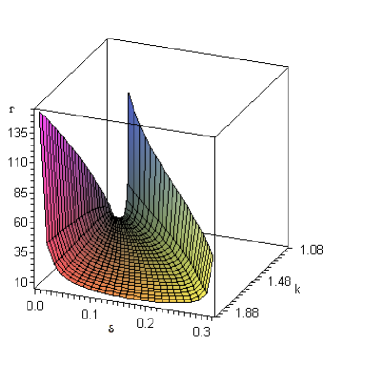
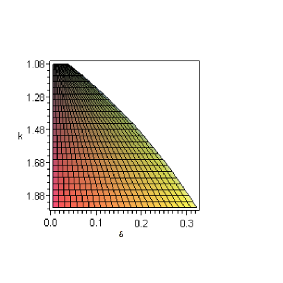
Figure 1: Left- Surface of Hopf bifurcation points in the $(\delta,\,k,\,r)$ space ($n=2$, $\beta_{0}=1$). Right- Projection of the surface on the plane $(k,\,\delta)$ -figures done with Maple.

Assuming that only one parameter varies (denote it by $\alpha$) while the others are kept fixed, a point $\alpha^{*},$ for which (11) is satisfied, is a nondegenerate Hopf bifurcation point if $\frac{d\mu}{d\alpha}(\alpha^{*})\neq 0$ and $l_{1}(\alpha^{*})\neq 0,$ where $l_{1}$ is the first Lyapunov coefficient, to be defined below. If $l_{1}(\alpha^{*})=0,$ the Hopf bifurcation is degenerate.

In the sequel we study the existence of points $\alpha^{**}$ in the parameter space, satisfying (9) and (10) and $l_{1}(\alpha^{**})=0,$ for the equilibrium point $x_{2}$. In order to do this, we have to construct an approximation of the local invariant center manifold and the approximation of the restriction of problem (1) to the local center manifold.

3.1 The center manifold, the restriction of the problem to the center manifold

In [7], by using the method of [3], the problem was formulated as an equation in the Banach space

$$\mathcal{B}_{0}=\left\{\psi:[-r,0]\mapsto\mathbb{R},\,\psi\,\mathrm{is\,continuous\,on\,}[-r,0)\wedge\,\exists\lim_{s\rightarrow 0}\psi(s)\in\mathbb{R}\right\},$$

that is

$$\frac{dz_{t}}{dt}=A(z_{t})+d_{0}\widetilde{f}(z_{t}),$$ (12)

where $\widetilde{f}(\varphi)=f(\varphi(0),\,\varphi(-r)),$

$$d_{0}(s)=\left\{\begin{array}[]{cc}0,&s\in[-r,0),\\ 1,&s=0,\\ \end{array}\right.$$

and, for $\varphi\in\mathcal{B}\subset\mathcal{B}_{0},$

$$A(\varphi)=\dot{\varphi}+d_{0}[L(\varphi)-\dot{\varphi}(0)],\;\;\;L(\varphi)=-(\delta+B_{1})\varphi(0)+kB_{1}\varphi(-r).$$ (13)

The developments of this subsection are done for a point $\alpha^{*},$ in the parameter space, for which relations (9) and (10) are satisfied. Hence the problem has two eigenvalues $\lambda_{1,2}=\pm i\omega^{*}$ and all other eigenvalues have strictly negative eigenvalues.

The eigenfunctions corresponding to eigenvalues $\lambda_{1,2}=\pm i\omega^{*}$ are given by $\varphi_{1,2}(s)=e^{\pm i\omega^{*}s},\,s\in[-r,0].$ Since the eigenfunctions are complex functions, we need to use the complexificates of the spaces $\mathcal{B},\,\mathcal{B}_{0}$ that we denote by $\mathcal{B}_{C},\,\mathcal{B}_{0C},$ respectively. We denote by $\mathcal{M}$ the subspace of $\mathcal{B}_{C}$ generated by $\varphi_{1,2}(\cdot).$

In [7], by using the ideas in [3], we constructed a projector $\mathcal{P}:\mathcal{B}_{0C}\mapsto\mathcal{M},$ that induces a projector defined on $\mathcal{B}_{C}$ with values also in $\mathcal{M}$. The space $\mathcal{B}_{C}$ is decomposed as a direct sum $\mathcal{M}\oplus\mathcal{N},$ where $\mathcal{N}=(I-\mathcal{P})\mathcal{B}_{C}.$ We do not present here the details of this construction. The projection of problem (1) on $\mathcal{M}$ leads us to the equation

$$\frac{du}{dt}=i\omega^{*}u+\Psi_{1}(0)\widetilde{f}(\varphi_{1}u+\varphi_{2}\overline{u}+\mathbf{v}),$$ (14)

where

$$\Psi_{1}(0)=\frac{1+(\delta+B_{1}-i\omega^{*})r}{[1+(\delta+B_{1})r]^{2}+\omega^{*2}r^{2}}.$$ (15)

The local center manifold is, for our problem, a $C^{\infty}$ invariant manifold, tangent to the space $\mathcal{M}$ at the point $z=0$ (that is $x=x_{2}$), and it is the graph of a function $w(\alpha^{*})(\cdot)$ defined on a neighborhood of zero in $\mathcal{M}$ and taking values in $\mathcal{N}$. A point on the local manifold has the form

$$u\,\varphi_{1}+\overline{u}\,\varphi_{2}+w(\alpha^{*})(u\,\varphi_{1}+\overline{u}\,\varphi_{2}).$$

The restriction of problem (1) with $x_{0}=\phi$ to the invariant manifold is

$$\frac{du}{dt}=\omega^{*}iu+\Psi_{1}(0)\widetilde{f}(\varphi_{1}u+\varphi_{2}\overline{u}+w(\alpha^{*})(u\varphi_{1}+\overline{u}\varphi_{2})),$$ (16)

with the initial condition $u(0)=u_{0},$ where $\mathcal{P}(\phi)=u_{0}\varphi_{1}+\overline{u}_{0}\varphi_{2}.$ The real and the imaginary parts of this complex equation, represent the two-dimensional restricted to the center manifold problem. We can study this problem with the tools of planar dynamical systems theory (see, e.g. [9]).

We set $\widetilde{w}(\alpha^{*})(u,\overline{u}):=w(\alpha^{*})(u(t)\varphi_{1}+\overline{u(t)}\varphi_{2}),$ and write

$$\widetilde{w}(\alpha^{*})(u,\overline{u})=\sum_{j+k\geq 2}\frac{1}{j!k!}w_{jk}(\alpha^{*})u^{j}\overline{u}^{k},$$ (17)

where $w_{jk}(\alpha^{*})\in\mathcal{B},$ $u:[0,\infty)\mapsto\mathbb{C}.$ By using (17), we write

$$\widetilde{f}(\varphi_{1}u+\varphi_{2}\overline{u}+w(\alpha^{*})(u\varphi_{1}+\overline{u}\varphi_{2}))=\sum_{j+k\geq 2}\frac{1}{j!k!}f_{jk}(\alpha^{*})u^{j}\overline{u}^{k}.$$ (18)

Equation (16) becomes

$$\frac{du}{dt}=\omega^{*}iu+\sum_{j+k\geq 2}\frac{1}{j!k!}g_{jk}(\alpha^{*})u^{j}\overline{u}^{k},$$ (19)

where

$$g_{jk}(\alpha^{*})=\Psi_{1}(0)f_{jk}(\alpha^{*}).$$ (20)

All the computation below are made at $\alpha=\alpha^{*}$ but, for simplicity, the parameter will not be written.

3.2 First Lyapunov coefficient

The first Lyapunov coefficient at $\alpha=\alpha^{*}$ is given by [9]

$$l_{1}=\frac{1}{2\omega^{*2}}Re(ig_{20}g_{11}+\omega^{*}g_{21}).$$ (21)

In order to compute it, we have to compute the corresponding coefficients $g_{jk},$ of (19), and, for this, we must find the coefficients of the series of $\widetilde{f}$ in (18).

We consider the function $q(x)=\beta(x)x,$ and its derivatives of order $n\geq 2$ in $x_{2},$ i.e. $B_{n}:=q^{(n)}(x_{2})=\beta^{(n)}(x_{2})x_{2}+n\beta^{(n-1)}(x_{2}).$ Let us also consider the function $F(x)=B_{2}x^{2}+B_{3}x^{3}+...+B_{n}x^{n}+...$ .

The nonlinear part of eq. (1) is

$$f(z(t),z(t-r))=-F(z(t))+kF(z(t-r)),$$

or, in terms of $z_{t},$ the function $\widetilde{f}$ of (12) is

$$\widetilde{f}(z_{t})=-F(z_{t}(0))+kF(z_{t}(-r)).$$

We denote by $\left\{\widetilde{T}(t)\right\}_{t\geq 0}$ the semigroup of operators generated by eq. (12). We have (by putting $\varphi_{1}=\varphi$, and by assuming that the initial function, $\phi,$ is on the invariant manifold)

$$\widetilde{f}(z_{t})=-F([\widetilde{T}(t)\phi](0))+kF([\widetilde{T}(t)\phi](-r))=$$ (22)

$$=-\frac{1}{2!}B_{2}[u\varphi(0)+\overline{u}\,\overline{\varphi}(0)+\frac{1}{2}w_{20}(0)u^{2}+w_{11}(0)u\overline{u}+\frac{1}{2}w_{02}(0)\overline{u}^{2}+...]^{2}-$$

$$-\frac{1}{3!}B_{3}[u\varphi(0)+\overline{u}\,\overline{\varphi}(0)+\frac{1}{2}w_{20}(0)u^{2}+w_{11}(0)u\overline{u}+\frac{1}{2}w_{02}(0)\overline{u}^{2}+...]^{3}-....+$$

$$+\frac{1}{2!}kB_{2}[u\varphi(-r)+\overline{u}\,\overline{\varphi}(-r)+\frac{1}{2}w_{20}(-r)u^{2}+w_{11}(-r)u\overline{u}+\frac{1}{2}w_{02}(-r)\overline{u}^{2}+...]^{2}+$$

$$+\frac{1}{3!}kB_{3}[u\varphi(-r)+\overline{u}\,\overline{\varphi}(-r)+\frac{1}{2}w_{20}(-r)u^{2}+w_{11}(-r)u\overline{u}+\frac{1}{2}w_{02}(-r)\overline{u}^{2}+...]^{3}+...=$$

$$=\sum_{j+k\geq 2}\frac{1}{j!k!}f_{jk}u^{j}\overline{u}^{k}.$$

The coefficients $f_{jk}$ involved in the expression of $l_{1},$ (computed also in [7]), are obtained by equating the same order terms in the two series from (22)

$$f_{20}=-B_{2}(1-ke^{-2\omega^{*}ir}),$$

$$f_{11}=B_{2}(k-1),$$

$$f_{02}=-B_{2}(1-ke^{2\omega^{*}ir}),$$

$$f_{21}=-B_{2}w_{20}(0)-2B_{2}w_{11}(0)+2kB_{2}e^{-i\omega^{*}r}w_{11}(-r)+kB_{2}e^{i\omega^{*}r}w_{20}(-r)-$$

$$-B_{3}(1-ke^{-i\omega^{*}r}),$$

from where $g_{ij}$ will be easily obtained from (20) (with $\Psi_{1}(0)$ given in (15)). Since $f_{21}$ depends on some values of $w_{20}$ and $w_{11}$, we have to determine these functions first.

The functions $w_{jk}\in\mathcal{B}_{C}$ are determined from the relation [14], [10], [5]

$$\frac{\partial}{\partial s}\sum_{j+k\geq 2}\frac{1}{j!k!}w_{jk}(s)u^{j}\overline{u}^{k}=\sum_{j+k\geq 2}\frac{1}{j!k!}g_{jk}u^{j}\overline{u}^{k}\varphi_{1}(s)+$$ (23)

$$+\sum_{j+k\geq 2}\frac{1}{j!k!}\overline{g}_{jk}\overline{u}^{j}u^{k}\varphi_{2}(s)+\frac{\partial}{\partial t}\sum_{j+k\geq 2}\frac{1}{j!k!}w_{jk}(s)u^{j}\overline{u}^{k},$$

that, by matching the same type terms yields differential equations for each $w_{jk}(s),$ while the integration constants are determined from

$$\frac{d}{dt}\sum_{j+k\geq 2}\frac{1}{j!k!}w_{jk}(0)u^{j}\overline{u}^{k}+\sum_{j+k\geq 2}\frac{1}{j!k!}g_{jk}u^{j}\overline{u}^{k}\varphi_{1}(0)+\sum_{j+k\geq 2}\frac{1}{j!k!}\overline{g}_{jk}\overline{u}^{j}u^{k}\varphi_{2}(0)=$$ (24)

$$-(B_{1}+\delta)\sum_{j+k\geq 2}\frac{1}{j!k!}w_{jk}(0)u^{j}\overline{u}^{k}+kB_{1}\sum_{j+k\geq 2}\frac{1}{j!k!}w_{jk}(-r)u^{j}\overline{u}^{k}+\sum_{j+k\geq 2}\frac{1}{j!k!}f_{jk}u^{j}\overline{u}^{k}.$$

E. g. in order to determine $w_{20}(s)$ we equate the terms containing $u^{2}$ and obtain

$$w^{\prime}_{20}(s)=2\omega^{*}iw_{20}(s)+g_{20}\varphi(s)+\overline{g}_{02}\overline{\varphi}(s).$$

We integrate between $-r$ and $0$ and obtain

$$w_{20}(0)-w_{20}(-r)e^{2\omega^{*}ir}=\frac{g_{20}i}{\omega^{*}}(1-e^{\omega^{*}ir})+\overline{g}_{02}\frac{i}{3\omega^{*}}(1-e^{3\omega^{*}ir}).$$

By equating the coefficients of $u^{2}$ in (24), the relation

$$\left(2\omega^{*}i+B_{1}+\delta\right)w_{20}(0)-kB_{1}w_{20}(-r)=f_{20}-g_{20}-\overline{g}_{02}$$

results. From the two relations above, we find $w_{20}(0)$ and $w_{20}(-r).$

The equations for all other functions $w_{ij}$ needed in the computation of $l_{1}$ and $l_{2}$ are all listed in the Appendix. They were obtained by symbolic computations in Maple.

Remark. The functions $w_{jk},\,j+k=2,$ were determined (for other problems) by many authors [1], [14], [10], in connection to the study of Hopf bifurcations.

Once $w_{20}(-r),\,w_{20}(0),\,w_{11}(-r),\,w_{11}(0)$ computed, we determine the value of $g_{21}$ and that of $l_{1}$.

The sign of the first Lyapunov coefficient $l_{1}$ determines the type of the Hopf bifurcation [9]. That is, if $l_{1}<0,$ we have a supercritical Hopf bifurcation, while if $l_{1}>0$ - a subcritical Hopf bifurcation.

4 Hopf points of codimension two

The Hopf points of codimension two are among the points of the surface of equation (11), surface that, for $n$ and $\beta_{0}$ fixed can be represented in $\mathbb{R}^{3}$ (as in Fig.1). Since they obey a new constraint, $l_{1}=0,$ they must lie on a curve on that surface. If we could write this constraint in a simple algebraical form, then we could attempt to represent the curve defined by (11) and $l_{1}=0.$ Unfortunately, this is not possible, since the expression of $l_{1},$ written in terms of the parameters of the problem is quite complex.

In this situation, our strategy for finding Hopf points of codimension two (Bautin type bifurcation points) is the following.

• As in [7], we chose $n^{*},\,\beta^{*}_{0},\,k^{*},\,\delta^{*},$ in a zone of parameters acceptable from biological point of view;

• with the chosen values of the parameters we compute $B^{*}_{1}$, (the value of $B_{1}$ at these parameters), next
  - if $B^{*}_{1}>0,$ then $x_{2}$ is stable for the chosen parameters and we stop;
  - if $B^{*}_{1}<0,$ we compute $p^{*}=\delta^{*}+B^{*}_{1},\,q^{*}=k^{*}B^{*}_{1}$;

• - if $|q^{*}|\leq|p^{*}|,$ we stop;
  - if $|q^{*}|>|p^{*}|,$ we determine $\omega^{*}$ and $r^{*}$ such that condition (9) is fulfilled i.e. we set $\omega^{*}=\sqrt{(q^{*})^{2}-(p^{*})^{2}},$ $r^{*}=\arccos(p^{*}/q^{*})/\omega^{*};$

• for the found values of parameters, the first Lyapunov coefficient, $l_{1}$, is computed;

• then we vary a parameter different of $r$, such that the absolute value of $l_{1}$ decreases - we have chosen to vary $\delta$;

• the above computations are repeated for several values of $\delta,$ until we find two values $\delta_{1},\,\delta_{2},$ of this parameter such that the values of $l_{1}$ have opposite signs - if such values exist (obviously, at each computation, the value of $r^{*}$ changes, but the condition $Re\lambda^{*}=0$ is maintained);

• then by using the bisection of the interval technique (with respect to $\delta$, starting from the interval $[\delta_{1},\,\delta_{2}]$), we find a set of parameters such that $l_{1}=0$ (to a certain approximation).

The obtained numerical results are presented in Section 5.

4.1 Second Lyapunov coefficient

In order to see if the Hopf points found by the above algorithm are points of codimension two, or have a higher degeneracy, we must compute the second Lyapunov coefficient in such a point.

The formula for the second Lyapunov coefficient, at a Hopf codimension two point is [9]

$$12l_{2}=\frac{1}{\omega^{*}}Reg_{32}+\frac{1}{\omega^{*2}}Im\left[g_{20}\overline{g}_{31}-g_{11}(4g_{31}+3\overline{g}_{22})-\frac{1}{3}g_{02}(g_{40}+\overline{g}_{13})-g_{30}g_{12}\right]+$$

$$+\frac{1}{\omega^{*3}}\left\{Re\left[g_{20}\left(\overline{g}_{11}(3g_{12}-\overline{g}_{30})+g_{02}(\overline{g}_{12}-\frac{1}{3}g_{30})+\frac{1}{3}\overline{g}_{02}g_{03}\right)+\right.\right.$$

$$\left.\left.+g_{11}\left(\overline{g}_{02}(\frac{5}{3}\overline{g}_{30}+3g_{12})+\frac{1}{3}g_{02}\overline{g}_{03}-4g_{11}g_{30}\right)\right]+3Im(g_{20}g_{11})Img_{21}\right\}+$$

$$+\frac{1}{\omega^{*4}}\left\{Im\left[g_{11}\overline{g}_{02}(\overline{g}^{2}_{20}-3\overline{g}_{20}g_{11}-4g_{11}^{2}\right]+Im(g_{20}g_{11})[3Re(g_{20}g_{11})-2|g_{02}|^{2}]\right\}.$$

We list below the expressions of the $f_{jk}$s corresponding to the involved $g_{jk}$s (not already given in Subsection 3.2):

$\;\,f_{30}=-3B_{2}w_{20}(0)-B_{3}+3kB_{2}e^{-i\omega^{*}r}w_{20}(-r)+kB_{3}e^{-3i\omega^{*}r},$

$\;\,f_{12}=\overline{f}_{21},\,f_{03}=\overline{f}_{30},$

$$\begin{array}[]{ccc}f_{40}&=&-B_{2}(3w_{20}(0)^{2}+4w_{30}(0))-6B_{3}w_{20}(0)-B_{4}+kB_{2}(3w_{20}(-r)^{2}+\\ &&+4e^{-i\omega r}w_{30}(-r))+6kB_{3}e^{-2i\omega r}w_{20}(-r)+kB_{4}e^{-4i\omega r},\\ &&\\ f_{31}&=&-B_{2}\left(3w_{11}(0)w_{20}(0)+3w_{21}(0)+w_{30}(0)\right)+B_{3}(3w_{11}(0)+3w_{20}(0))-\\ &&-B_{4}+kB_{2}(3w_{11}(-r)w_{20}(-r)+3e^{-i\omega r}w_{21}(-r)+e^{i\omega r}w_{30}(-r))+\\ &&+kB_{3}(3e^{-2i\omega r}w_{11}(-r)+3w_{20}(-r))+kB_{4}e^{-2\omega ir},\\ &&\\ f_{22}&=&-B_{2}(2w_{11}(0)^{2}+2w_{12}(0)+w_{02}(0)w_{20}(0)+2w_{21}(0))+B_{3}(w_{02}(0)+\\ &&+4w_{11}(0)+w_{20}(0))-B_{4}+kB_{2}(2w_{11}(-r)^{2}+2e^{-i\omega r}w_{12}(-r)+\\ &&+w_{02}(-r)w_{20}(-r)+2e^{i\omega r}w_{21}(-r))+kB_{3}(w_{02}(-r)e^{-2i\omega r}+\\ &&+4w_{11}(-r)+e^{2i\omega r}w_{20}(-r))+kB_{4};\end{array}$$

$\;\,f_{04}=\overline{f}_{40},\,f_{31}=\overline{f}_{31},$ and, finally,

$$\begin{array}[]{ccc}f_{32}=&-B_{2}\left[w_{02}(0)w_{30}(0)+6w_{11}(0)w_{21}(0)+3w_{22}(0)+3w_{12}(0)w_{20}(0)+\right.\\ &\left.+2w_{31}(0)\right]-B_{3}\left[6w_{11}(0)^{2}+3w_{12}(0)+3w_{02}(0)w_{20}(0)+w_{30}(0)+\right.\\ &\left.+6w_{11}(0)w_{20}(0)+6w_{21}(0)\right]+B_{4}\left[3w_{20}(0)+6w_{11}(0)+w_{02}(0)\right]-\\ &-B_{5}+kB_{2}\left[6w_{11}(-r)w_{21}(-r)+3w_{12}(-r)w_{20}(-r)+3e^{-i\omega r}w_{22}(-r)+\right.\\ &\left.+w_{02}(-r)w_{30}(-r)+2e^{i\omega r}w_{31}(-r)\right]+kB_{3}\left[3w_{02}(-r)e^{-i\omega r)}w_{20}(-r)+\right.\\ &+6e^{-i\omega r}w_{11}(-r)^{2}+3e^{-2i\omega r}w_{12}(-r)+e^{2i\omega r}w_{30}(-r)+\\ &\left.+6e^{i\omega r}w_{11}(-r)w_{20}(-r)+6w_{21}(-r)\right]+kB_{4}\left[3e^{i\omega r}w_{20}(-r)+\right.\\ &\left.+6e^{-i\omega r}w_{11}(-r)+w_{02}(-r)e^{-3i\omega r}\right]+kB_{5}e^{-i\omega r}.\end{array}$$

The values in 0 and $-r$ of the involved $w_{ij}$s are computed by solving the differential equations and by using the additional conditions listed in the Appendix.

There is a function $w_{jk}$ that requires a special treatment, i.e. $w_{21}$. As shown in [8], the two equations that determine $w_{21}(0),\,w_{21}(-r)$ are dependent, and the value of $w_{21}(0)$ may be obtained by considering a perturbed problem (depending on a small $\epsilon$), computing the corresponding $w_{\epsilon 21}$ and by taking the limit as $\epsilon\rightarrow 0.$ The formula obtained in [8] is

$$w_{21}(0)=\frac{f_{21}\langle\Psi_{1}+\Psi_{2},\,\rho\rangle-2g_{11}\langle\widetilde{\rho},w_{20}\rangle-(g_{20}+2\overline{g}_{11})\langle\widetilde{\rho},w_{11}\rangle-\overline{g}_{02}\langle\widetilde{\rho},w_{02}\rangle}{2r\omega i-2rA+2},$$ (25)

where $\langle,\,\rangle$ is the bilinear form [3], [4], [7] defined on $C([0,r],\mathbb{R})\times C([-r,0],\mathbb{R}),$ by

$$\langle\psi,\varphi\rangle=\psi(0)\varphi(0)+kB_{1}\int_{-r}^{0}\psi(\zeta+r)\varphi(\zeta)d\zeta,$$ (26)

$\rho(s)=-2se^{\omega is},\;s\in[-r,0]$ and $\widetilde{\rho}(\zeta)=-2\zeta e^{-\omega i\zeta},\;\zeta\in[0,r].$

After determining $w_{21}(0),$ we compute $w_{21}(-r)$ by using any of the two relations that connect the two values. All other necessary values of $w_{jk}$, $j+k\leq 4$ are determined by using the relations in the Appendix.

5 Results

As we asserted above, we explored the equilibrium point $x_{2}$ with regard to the occurrence of Hopf degenerate bifurcations. As first step we search for points in the parameter space, where $l_{1}=0.$

We explored the zone of parameters $(n,\,\beta_{0},\,k)$ given by:

$$(n,\,\beta_{0},\,k)\in\{1,1.5,2,3,...,12\}\times\{0.5,1,1.5,2,2.5\}\times\{1.1,1.2,...,1.9\}$$

(we remind that $k>1$ in order that $x_{2}$ exist, and $k<2$).

For every $(n^{*},\beta^{*}_{0},k^{*})$ fixed, we looked for a $\delta^{*}$ and a $r^{*}$ such that $Re\lambda_{1,2}(\alpha^{*})=0$ and $l_{1}=0.$

We easily see that the case $\mathbf{n=1}$ is not interesting since, for $n=1,$ by (5), $B_{1}=\frac{\delta^{2}}{\beta_{0}(k-1)^{2}}>0,$ and the points with $B_{1}>0$ are points where $x_{2}$ is stable and no Hopf bifurcations can occur.

Interesting results were found for $\mathbf{n=1.5}$ and $\mathbf{n=2}.$ For each $\beta_{0}\in\{0.5,\,1,\,1.5,\,2,\,2.5\},$ and each $k\in\{1.1,\,1.2,...,1.9\}$ we encountered the following behavior: at small values of $\delta$ (i.e. $\delta=0.0001$), we found $B_{1}<0,$ hence we could detect Hopf points. For these points $l_{1}$ was proved to be positive, it decreased with increasing $\delta$ and became negative for some value of $\delta$. We then applied the bisection of interval technique as described in Section 4.1 and actually found Hopf points with $l_{1}=0$.

For each such points we computed the second Lyapunov coefficient and we found that all points with $l_{1}=0,$ determined before, have $l_{2}<0,$ hence they are codimension two Hopf points.

For $n=1.5$ the Hopf points occur for very large values of $r$ ($r>60$) and, since such values for $r$ are not realistic (as asserted in [11], [12]), we present only the results obtained for $n=2.$

In Figures 2-6 we present the sets of parameters $\alpha^{**}$ with $l_{1}(\alpha^{**})=0$ found by us, in tables and plotted on the surfaces of Hopf bifurcation points. These points were determined as the points where $|l_{1}|$ is approximately equal to $10^{-10}.$ A better precision may be attained by continuing the bisection interval procedure further.

k	$\delta$	$r$	$l_{2}$
1.1	0.0045705962	26.125314	-0.021
1.2	0.0090491351	25.751524	-0.0151
1.3	0.0134437887	25.422162	-0.0124
1.4	0.0177612407	25.130258	-0.0108
1.5	0.0220070315	24.870352	-0.0097
1.6	0.0261858065	24.638093	-0.0088
1.7	0.0303014988	24.429962	-0.0081
1.8	0.0343574676	24.243076	-0.0076
1.9	0.0383566021	24.075039	-0.0071

Figure 2: Hopf codimension two points for $n=2,\,\beta_{0}=0.5.$

k	$\delta$	$r$	$l_{2}$
1.1	0.0091411924	13.062657	-0.0205
1.2	0.0180982702	12.875762	-0.0142
1.3	0.0268875774	12.711081	-0.0114
1.4	0.0355224814	12.565129	-0.0097
1.5	0.0440140630	12.435176	-0.0085
1.6	0.0523716129	12.319046	-0.0076
1.7	0.0606029975	12.214981	-0.0069
1.8	0.0687149345	12.121538	-0.0063
1.9	0.0767132043	12.037519	-0.0059

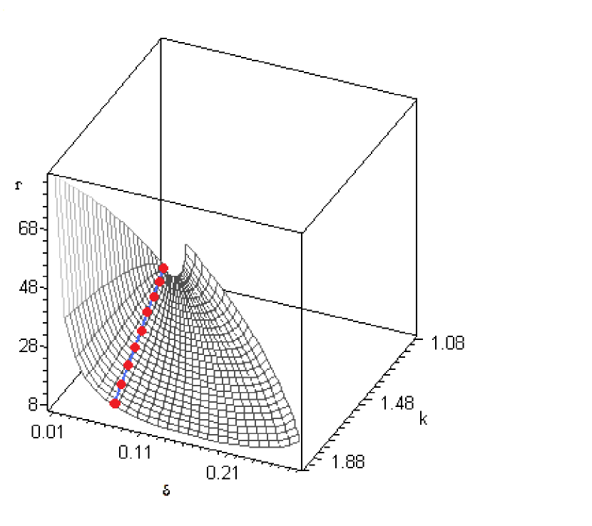
Figure 3: Hopf codimension two points for $n=2,\,\beta_{0}=1.$

k	$\delta$	$r$	$l_{2}$
1.1	0.0137117887	8.708438	-0.0204
1.2	0.0271474053	8.583841	-0.0140
1.3	0.0403313662	8.474054	-0.0112
1.4	0.0532837222	8.376752	-0.0095
1.5	0.0660210946	8.290117	-0.0083
1.6	0.0785741932	8.212697	-0.0074
1.7	0.0909044966	8.143320	-0.0067
1.8	0.1030724022	8.081025	-0.0061
1.9	0.1150698062	8.025013	-0.0056

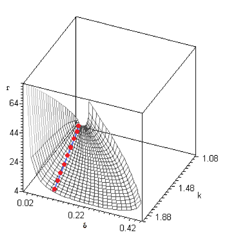
Figure 4: Hopf codimension two points for $n=2,\,\beta_{0}=1.5.$

k	$\delta$	$r$	$l_{2}$
1.1	0.018282385	6.531328	-0.0203
1.2	0.036196540	6.437880	-0.014
1.3	0.053775154	6.355540	-0.0111
1.4	0.071044963	6.282564	-0.0093
1.5	0.088028126	6.217588	-0.0082
1.6	0.104743225	6.159523	-0.0073
1.7	0.121205995	6.107490	-0.0066
1.8	0.137429869	6.060769	-0.0060
1.9	0.153426408	6.018759	-0.0055

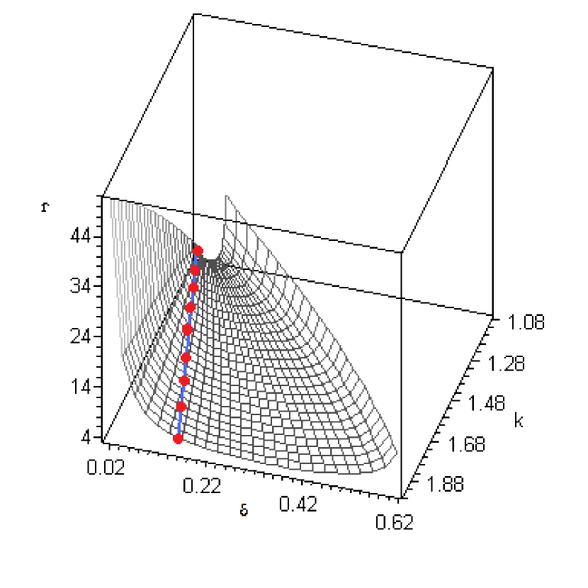
Figure 5: Hopf codimension two points for $n=2,\,\beta_{0}=2.$

k	$\delta$	$r$	$l_{2}$
1.1	0.022852981	5.225062	-0.0203
1.2	0.045245675	5.150304	-0.0139
1.3	0.067218943	5.084432	-0.0110
1.4	0.088806203	5.026051	-0.0093
1.5	0.110035157	4.974074	-0.0081
1.6	0.130929032	4.927618	-0.0073
1.7	0.151507494	4.885992	-0.0066
1.8	0.171787337	4.848615	-0.0060
1.9	0.191783010	4.815007	-0.0055

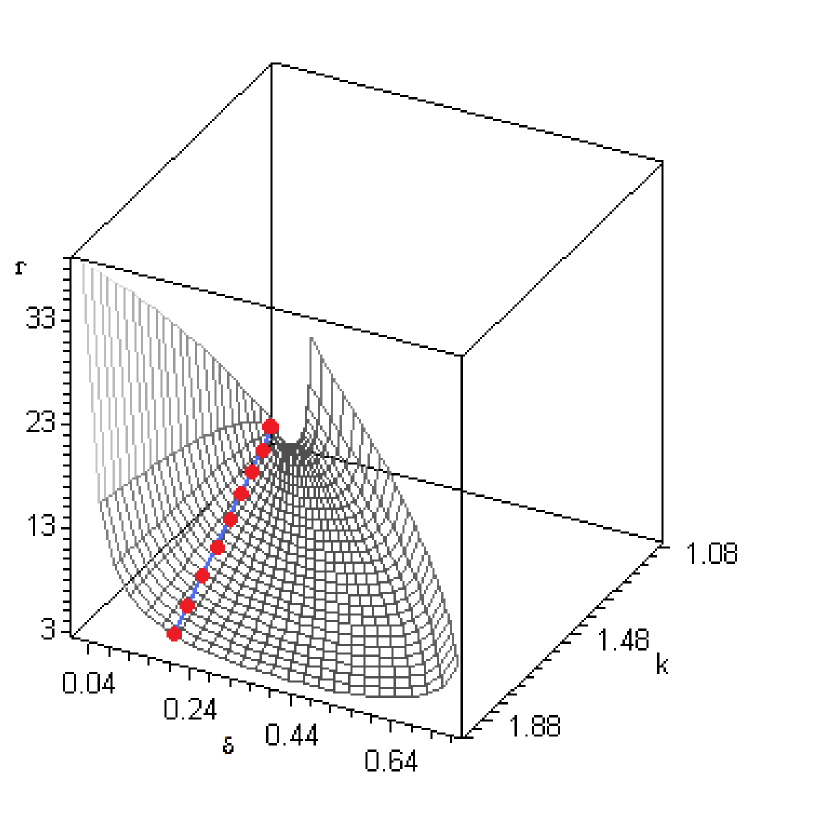
Figure 6: Hopf codimension two points for $n=2,\,\beta_{0}=2.5.$

By connecting the points with $l_{1}=0$ we determine approximately a curve of points with $l_{1}=0$ on each of the surfaces in Figs. 2-6. Let us denote by $\delta=\widetilde{\delta}(k)$ the projection of this curve on the plane $(k,\,\delta)$. Our computations of $l_{1}$ showed that on each of the surfaces in Figs. 2-6, $l_{1}>0$ for the points of the surface that are projected on the zone $\delta<\widetilde{\delta}(k)$ of the plane $(k,\,\delta)$, and hence in this zone, the Hopf bifurcation is subcritical. For the points that are projected on the zone $\delta>\widetilde{\delta}(k)$ we found $l_{1}<0$, hence in this zone, the Hopf bifurcation is supercritical.

Finally, for $\mathbf{3\leq n\leq 12}$ the Hopf points found had only negative $l_{1},$ and thus, we could not find any degenerate Hopf points.

6 Conclusions

The existence of Hopf codimension two points was investigated for the non-zero equilibrium point of the equation that models the periodic chronic myelogenous leukemia, presented in [12], [11]. We searched such points in a zone of the 5-dimensional parameters space, of biological significance. We found that points $\alpha$ with $l_{1}(\alpha)=0$ actually exist and we present tables with values of the parameters where they occur. For each of these points we computed the corresponding second Lyapunov coefficient $l_{2}(\alpha)$ and listed the obtained values in the above mentioned tables. We remark that for all the considered sets of parameters, $l_{2}<0.$ We also remark that the values of $l_{2}$ are close to zero, and, at least for $n=2$ and the chosen values of $\beta_{0}$ the behavior of $l_{2}$ as function of $k$ is the same, i.e. $l_{2}$ decreases when $k$ increases. Since $k=2e^{-\gamma r},$ it can not be greater than 2, and for $k<2$ we found only negative values of $l_{2}$ (we also considered in our computation the limit case $k=2$ - that would imply $\gamma=0$ - and for $n=2,\,k=2$ and for every $\beta_{0}$ considered we found still negative $l_{2}$ in the points where $l_{1}=0$). Hence among the considered points no higher order degeneracies can be found (in the zones with biological significance).

The points where $l_{1}=0$ and $l_{2}\neq 0$ are, if we vary two parameters, points of Bautin bifurcation (provided a certain non-degeneracy condition is satisfied [5]). A numerical investigation of the solutions of the equation for the parameters in and around the points with $l_{1}=0,$ is in course and will be soon submitted to publication.

7 APPENDIX

We list below the differential equations, their solutions, and the supplementary conditions for the functions $w_{jk}$ with $j+k\leq 4,$ excepting $w_{20}$ that is treated in Section 3. The right hand side of the differential equations as well as the supplementary conditions are obtained by symbolic computation in Maple.

$\mathbf{w_{11}:}$

$$\frac{dw_{11}(s)}{ds}=g_{11}e^{i\omega s}+\overline{g}_{11}e^{-i\omega s},$$

$$w_{11}(s)=w_{11}(0)-\frac{ig_{11}}{\omega}(e^{\omega is}-1)+\frac{i\overline{g}_{11}}{\omega}(e^{-\omega is}-1),$$

$$(B_{1}+\delta)w_{11}(0)-kB_{1}w_{11}(-r)=f_{11}-g_{11}-\overline{g}_{11}.$$

For $\mathbf{w_{02}}$, we have $w_{02}=\overline{w}_{20}$.

$\mathbf{w_{30}:}$

$$\frac{dw_{30}(s)}{ds}=3\omega iw_{30}(s)+g_{30}e^{i\omega s}+\overline{g}_{03}e^{-i\omega s}+3g_{20}w_{20}(s)+3\overline{g}_{02}w_{11}(s),$$

$$w_{30}(s)=w_{30}(0)e^{3\omega is}+\frac{i}{2\omega}g_{30}(e^{i\omega s}-e^{3\omega is})+\frac{i}{4\omega}\overline{g}_{03}(e^{-i\omega s}-e^{3\omega is})+3g_{20}e^{3\omega is}\int_{0}^{s}w_{20}(\theta)e^{-3\omega i\theta}d\theta+$$

$$+3\overline{g}_{02}e^{3\omega is}\int_{0}^{s}w_{11}(\theta)e^{-3\omega i\theta}d\theta,$$

$$(3\omega i+B_{1}+\delta)w_{30}(0)-kB_{1}w_{30}(-r)=f_{30}-g_{30}-\overline{g}_{03}-3g_{20}w_{20}(0)-3\overline{g}_{02}w_{11}(0).$$

$\mathbf{w_{21}:}$

$$\frac{dw_{21}(s)}{ds}=\omega iw_{21}(s)+g_{21}e^{i\omega s}+\overline{g}_{12}e^{-i\omega s}+2g_{11}w_{20}(s)+(g_{20}+2\overline{g}_{11})w_{11}(s)+\overline{g}_{02}w_{02}(s),$$

$$w_{21}(s)=w_{21}(0)e^{\omega is}+g_{21}se^{\omega is}+\frac{i}{2\omega}\overline{g}_{12}(e^{-i\omega s}-e^{\omega is})+2g_{11}e^{\omega is}\int_{0}^{s}w_{20}(\theta)e^{-i\omega\theta}d\theta+$$

$$+(g_{20}+2\overline{g}_{11})e^{\omega is}\int_{0}^{s}w_{11}(\theta)e^{-i\omega\theta}d\theta+\overline{g}_{02}e^{\omega is}\int_{0}^{s}w_{02}(\theta)e^{-i\omega\theta}d\theta,$$

$$(\omega i+B_{1}+\delta)w_{21}(0)-kB_{1}w_{21}(-r)=f_{21}-g_{21}-\overline{g}_{12}-2g_{11}w_{20}(0)-(g_{20}+2\overline{g}_{11})w_{11}(0)-\overline{g}_{02}w_{02}(0).$$

$\mathbf{w_{03}:}$ $w_{03}=\overline{w}_{30}.$
$\mathbf{w_{12}:}$ $w_{12}=\overline{w}_{21}.$

$\mathbf{w_{40}:}$

$$\frac{dw_{40}(s)}{ds}=g_{40}e^{i\omega s}+\overline{g}_{04}e^{-i\omega s}+4\omega iw_{40}(s)+4g_{30}w_{20}(s)+4\overline{g}_{03}w_{11}(s)+6g_{20}w_{30}(s)+6\overline{g}_{02}w_{21}(s),$$

$$w_{40}(s)=w_{40}(0)e^{4\omega is}+\frac{i}{3}g_{40}(e^{i\omega s}-e^{4\omega is})+\frac{i}{5}\overline{g}_{04}(e^{-i\omega s}-e^{4\omega is})+4g_{30}e^{4\omega is}\int_{0}^{s}w_{20}(\theta)e^{-4\omega i\theta}d\theta+$$

$$+4\overline{g}_{03}e^{4\omega is}\int_{0}^{s}w_{11}(\theta)e^{-4\omega i\theta}d\theta+6g_{20}e^{4\omega is}\int_{0}^{s}w_{30}(\theta)e^{-4\omega i\theta}d\theta+6\overline{g}_{02}e^{4\omega is}\int_{0}^{s}w_{21}(\theta)e^{-4\omega i\theta}d\theta,$$

$$(4\omega i+B_{1}+\delta)w_{40}(0)-kB_{1}w_{40}(-r)=f_{40}-g_{40}-\overline{g}_{04}-4g_{30}w_{20}(0)-4\overline{g}_{03}w_{11}(0)-$$

$$-6g_{20}w_{30}(0)-6\overline{g}_{02}w_{21}(0).$$

$\mathbf{w_{31}:}$

$$\frac{dw_{31}(s)}{ds}=2\omega iw_{31}(s)+g_{31}e^{i\omega s}+\overline{g}_{13}e^{-i\omega s}+3g_{21}w_{20}(s)+(3\overline{g}_{12}+g_{30})w_{11}(s)+$$

$$+\overline{g}_{03}w_{02}(s)+3g_{11}w_{30}(s)+3(g_{20}+\overline{g}_{11})w_{21}(s)+3\overline{g}_{02}w_{12}(s),$$

$$w_{31}(s)=w_{31}(0)e^{2\omega is}+\frac{i}{\omega}g_{31}(e^{i\omega s}-e^{2\omega is})+\frac{i}{3\omega}\overline{g}_{13}(e^{-i\omega s}-e^{2\omega is})+3g_{21}e^{2\omega is}\int_{0}^{s}w_{20}(\theta)e^{-2\omega i\theta}d\theta+$$

$$+(g_{30}+3\overline{g}_{12})e^{2\omega is}\int_{0}^{s}w_{11}(\theta)e^{-2\omega i\theta}d\theta+\overline{g}_{03}e^{2\omega is}\int_{0}^{s}w_{02}(\theta)e^{-2\omega i\theta}d\theta+$$

$$+3g_{11}e^{2\omega is}\int_{0}^{s}w_{30}(\theta)e^{-2\omega i\theta}d\theta+(3\overline{g}_{11}+3g_{20})e^{2\omega is}\int_{0}^{s}w_{21}(\theta)e^{-2\omega i\theta}d\theta+3\overline{g}_{02}e^{2\omega is}\int_{0}^{s}w_{12}(\theta)e^{-2\omega i\theta}d\theta,$$

$$(2\omega i+B_{1}+\delta)w_{31}(0)-kB_{1}w_{31}(-r)=f_{31}-g_{31}-\overline{g}_{13}-3g_{21}w_{20}(0)-(g_{30}+3\overline{g}_{12})w_{11}(0)-$$

$$-\overline{g}_{03}w_{02}(0)-3g_{11}w_{30}(0)-3(g_{20}+\overline{g}_{11})w_{21}(0)-3\overline{g}_{02}w_{12}(0).$$

$\mathbf{w_{22}:}$

$$\frac{dw_{22}(s)}{ds}=g_{22}e^{i\omega s}+\overline{g}_{22}e^{-i\omega s}+2g_{12}w_{20}(s)+2(g_{21}+\overline{g}_{21})w_{11}(s)+2\overline{g}_{12}w_{02}(s)+$$

$$+g_{02}w_{30}(s)+(4g_{11}+\overline{g}_{20})w_{21}(s)+(g_{20}+4\overline{g}_{11})w_{12}(s)+\overline{g}_{02}w_{03}(s),$$

$$w_{22}(s)=w_{22}-\frac{i}{\omega}g_{22}(e^{i\omega s}-1)+\frac{i}{\omega}\overline{g}_{22}(e^{-i\omega s}-1)+2g_{12}\int_{0}^{s}w_{20}(\theta)d\theta+$$

$$+2(g_{21}+\overline{g}_{21})\int_{0}^{s}w_{11}(\theta)d\theta+2\overline{g}_{12}\int_{0}^{s}w_{02}(\theta)d\theta+g_{02}\int_{0}^{s}w_{30}(\theta)d\theta+$$

$$+(\overline{g}_{20}+4g_{11})\int_{0}^{s}w_{21}(\theta)d\theta+(g_{20}+4\overline{g}_{11})\int_{0}^{s}w_{12}(\theta)d\theta+\overline{g}_{02}\int_{0}^{s}w_{03}(\theta)d\theta,$$

$$(B_{1}+\delta)w_{22}(0)-kB_{1}w_{22}(-r)=f_{22}-g_{22}+\overline{g}_{22}-2g_{12}w_{20}(0)-2(g_{21}+\overline{g}_{21})w_{11}(0)-$$

$$-2\overline{g}_{12}w_{02}(0)-g_{02}w_{30}(0)-(4g_{11}+\overline{g}_{20})w_{21}(0)-(g_{20}+4\overline{g}_{11})w_{12}(0)-\overline{g}_{02}w_{03}(0).$$

$\mathbf{w_{13}:}$ $w_{13}=\overline{w}_{31}.$
$\mathbf{w_{04}:}$ $w_{04}=\overline{w}_{40}.$

Author’s addresses:

Anca-Veronica Ion,

”Gh. Mihoc-C. Iacob” Institute of Mathematical Statistics

and Applied Mathematics of the Romanian Academy,

Calea 13 Septembrie nr. 13, 050711, Bucharest, Romania.

e-mail address: anca-veronica.ion@ima.ro

Raluca Mihaela Georgescu,

Faculty of Mathematics and Computer Sciences,

Târgu din Vale, nr. 1, 110040, Piteşti, Argeş.

e-mail address: gemiral@yahoo.com

References

• [1] S. A. Campbell, Calculating centre manifolds for delay differential equations using Maple, In Balachandran B., Kalmar Nagy T. and Gilsinn D. (eds), Delay Differential Equations: Recent Advances and New Directions, Springer, New York, 2009.
• [2] N. D. Hayes, Roots of the transcendental equation associated with a certain difference-differential equation, J. London Math. Soc., 1950, 226-232.
• [3] T. Faria, Normal forms for RFDE in finite dimensional spaces -section 8.3 of J. Hale, L.T. Magalhaez, W. Oliva, Dynamics in infinite dimensions, Applied Mathematical Sciences, 47, Springer, New York, 2002.
• [4] J. Hale, S. M. Verduyn Lunel, Introduction to functional differential equation, Applied Mathematical Sciences, 99, Springer, New York, 2003.
• [5] A. V. Ion, On the Bautin bifurcation for systems of delay differential equations, Acta Univ. Apulensis, 8(2004), 235-246 (Proc. of ICTAMI 2004, Thessaloniki, Greece); arXiv:1111.1559.
• [6] A. V. Ion, New results concerning the stability of equilibria of a delay differential equation modeling leukemia, Proceedings of The 12th Symposium of Mathematics and its Applications, Timişoara, November 5-7, 2009, 375-380; arXiv:1001.4658.
• [7] A. V. Ion, R. M. Georgescu, Stability of equilibrium and periodic solutions of a delay equation modeling leukemia, Works of the Middle Volga Mathematical Society, 11(2009); arXiv:1001.5354.
• [8] A. V. Ion, On the computation of the third order terms of the series defining the center manifold for a scalar delay differential equation, accepted in Journal of Dynamics and Differential Equations, DOI 10.1007/s10884-012-9243-8.
• [9] Y. A. Kuznetsov, Elements of applied bifurcation theory, Applied Mathematical Sciences, 112, Springer, New York, 1998.
• [10] G. Mircea, M. Neamţu, D. Opriş, Dynamical systems from economy, mechanics, biology, described by delay equations, Mirton, Timişoara, 2003 (in Romanian).
• [11] L. Pujo-Menjouet, M. C. Mackey, Contribution to the study of periodic chronic myelogenous leukemia, C. R. Biologies, 327(2004), 235-244.
• [12] L. Pujo-Menjouet, S. Bernard, M. C. Mackey, Long period oscillations in a $G_{0}$ model of hematopoietic stem cells, SIAM J. Applied Dynamical Systems, 2, 4(2005), 312-332.
• [13] J. Sotomayor, L.F. Mello, D. C.Braga, Lyapunov Coefficients for Degenerate Hopf Bifurcations, arXiv: 0709.3949.
• [14] Wischert W., Wunderlin A., Pelster A., Olivier M., Groslambert J, Delay induced instabilities in nonlinear feedback syatems, Physical Review E, 49, 1(1994), 203-219.