Spectroscopy of extended Ly$\alpha$ envelopes around $z=4.5$ quasars

What are the frequency, shape, kinematics, and luminosity of Ly$\alpha$ envelopes surrounding radio-quiet quasars at high redshift, and is the luminosity of these envelopes related to that of the quasar or not? As a first step towards answering these questions, we have searched for Ly$\alpha$ envelopes around six radio-quiet quasars at $z\sim 4.5$, using deep spectra taken with the FORS2 spectrograph attached to the UT1 of the Very Large Telescope (VLT). Using the multi-slit mode allows us to observe several point spread function stars simultaneously with the quasar, and to remove the point-like emission from the quasar, unveiling the faint underlying Ly$\alpha$ envelope with unprecedented depth. An envelope is detected around four of the six quasars, which suggests that these envelopes are very frequent. Their diameter varies in the range $26\lesssim d\lesssim 64$ kpc, their surface brightness in the range $3\times 10^{-19}\lesssim\mu\lesssim 2\times 10^{-17}$ erg s^-1 cm^-2 arcsec^-2 , and their luminosity in the range $10^{42}\lesssim L(Ly\alpha)\lesssim 10^{44}$ erg s^-1 . Their shape may be strongly asymmetric. The Ly$\alpha$ emission line full width at half maximum (FWHM) is $900<FWHM<2200$  km s^-1and its luminosity correlates with that of the broad line region (BLR) of the quasar, with the notable exception of BR2237-0607, the brightest object in our sample. The same holds for the relation between the envelope Ly$\alpha$ luminosity and the ionizing luminosity of the quasar. While the deep slit spectroscopy presented in this paper is very efficient at detecting very faint Ly$\alpha$ envelopes, narrow-band imaging is now needed to measure accurately their spatial extent, radial luminosity profile, and total luminosity. These observables are crucial to help us discriminate between the three possible radiation processes responsible for the envelope emission: (i) cold accretion, (ii) fluorescence induced by the quasar, and (iii) scattering of the BLR photons by cool gas.

1 Introduction

The so-called “Ly$\alpha$ blobs” have attracted much attention in the past few years. They are extended nebulae at high redshift ($z\sim 2-5$) emitting in the Ly$\alpha$ line, with typical sizes of $\sim 10\arcsec$ or $\sim 100$ kpc (Steidel et al., 2000; Matsuda et al., 2004, 2011; Yang et al., 2009). Their Ly$\alpha$ luminosity is typically $\sim 10^{43}$ erg s^-1 , and, while they are numerous at high redshift, they seem to disappear at moderate to low redshift (Keel et al., 2009). The source of their power has remained unclear and a controversial subject. Some host an active galactic nucleus (AGN) at their centre, while others apparently do not (Geach et al., 2009; Yang et al., 2009). Recently, extended Ly$\alpha$ emission was discovered around the $z=6.4$ radio-quiet quasar CFHQSJ2329-0301 (Willott et al., 2011; Goto et al., 2012).

Extended Ly$\alpha$ emission has also been observed around high-redshift radio galaxies (Heckman et al., 1991a; van Ojik et al., 1996), as well as around radio-quiet quasars (Christensen et al. 2006; Bunker et al. 2003). The Ly$\alpha$ flux from the nebula is about 0.5% of the flux in the integrated broad Ly$\alpha$ line of the QSO, in the case of radio-quiet quasars (RQQs). For radio-loud quasars (RLQs) or radio-galaxies, the Ly$\alpha$ flux of the nebula is an order of magnitude higher (Christensen et al., 2006), presumably because the emission of RLQ gaseous envelopes is enhanced by interactions with the radio jets. In addition, it seems that the RLQs generally reside in richer environments than RQQs (Ellison et al., 2002).

Two main power sources have been suggested to explain the luminosity of the Ly$\alpha$ blobs (excluding the envelopes of RLQs). The first is photo-ionization by a central source such as an AGN or a starburst region (e.g. Chelouche et al., 2008). Geach et al. (2009) recently presented arguments in favour of this idea, based on deep X-ray observations of Ly$\alpha$ blobs. They unveiled obscured AGNs but found no diffuse X-ray emission that would have betrayed the existence of a hot gas component with $T\gtrsim 10^{7}$ K; the lack of such a component rules out inverse Compton scattering of CMB photons as an ionizing source. The other possible power source is cold accretion, a scenario where pristine gas falling into the potential well of a dark matter halo gets heated and ionized by collisions, converting gravitational energy into Ly$\alpha$ radiation. According to Dijkstra & Loeb (2009), observed Ly$\alpha$ blobs could be explained in this way if only $\gtrsim 10$% of the gravitational binding energy of cold gas being accreted onto a galaxy is converted into Ly$\alpha$ radiation (such a conversion was also discussed by Haiman et al. 2000 and by Fardal et al., 2001). In addition, since the emission would come from filamentary cold flows, it would not depend on the existence of a central ionizing source such as an AGN, because the cold gas would be self-shielded from the ionizing radiation.

A blind search for Ly$\alpha$ blobs has the advantage of providing a bias-free sample, but is very time-consuming. It requires wide-field, narrow-band imaging, and the candidates found in this way still have to be observed spectroscopically to be confirmed. Alternatively, looking for Ly$\alpha$ blobs around radio-quiet quasars takes advantage of pre-existing catalogues. In addition, bright quasars are thought to reside in massive halos ($\sim 5\times 10^{12}$ M_⊙ , see e.g. Hopkins et al., 2007), which are also thought to host the so-called “cold flows” (Kereš et al., 2009) that could emit a substantial Ly$\alpha$ flux (Dijkstra & Loeb, 2009). The main drawbacks of this alternative search technique are that (1) it is not guaranteed a priori that a Ly$\alpha$ nebula is present around each quasar, (2) the sample will inevitably be biased, and (3) the bright quasar emission has to be subtracted before one can see and characterize the Ly$\alpha$ envelope.

We initiated, a few years ago, a pilot survey aimed at exploring in detail the spatial extent, the luminosity and kinematics of the large hydrogen envelopes of remote quasars spanning a broad magnitude range, at redshift $z\sim 4.5$. In this way, the possible relation between the quasar luminosity and the extent and luminosity of the envelope could be explored. In a model where photoionization by the AGN is the main cause of the Ly$\alpha$ luminosity (e.g. Haiman & Rees, 2001), one should expect the latter to be strongly correlated with the luminosity of the quasar, at least that coming from the ionizing Lyman continuum. Alternatively, in the model of Dijkstra & Loeb (2009), no direct relation between the AGN luminosity and that of the blob is expected. Preliminary results of our survey have been published (Courbin et al., 2008, Paper I) for three quasars, one of which is surrounded by a Ly$\alpha$ envelope (it appears that the marginal detection of a second one was spurious); the observational strategy was explained in more details in that paper. The present article describes our detection of a Ly$\alpha$  nebula around two more quasars, and a marginal detection around a sixth one. The observations are described in Section 2 and the results are presented in Section 3. The results are discussed assuming a cosmology with $H_{0}=72$  km s^-1 Mpc^-1 , $\Omega_{M}=0.3$, and $\Omega_{\lambda}=0.7$.

Table 1: Journal of observations and main characteristics of the quasars.

Name	JD(start)	Exposure	Airmass	Seeing
	$-2400000$	time (s)	(start)	(”)
SDSS J14472+0401, z=4.580, R(AB)=19.9$\pm$0.2, MR=-28.2
	54647.617	1300	1.30	$0.54$
	54647.633	1300	1.38	$0.57$
	54653.565	1300	1.18	$0.61$
	54653.581	1300	1.22	$0.60$
	54654.562	1300	1.18	$0.85$
	54654.577	1300	1.22	$0.88$
	54654.600	1300	1.31	$0.89$
	54654.615	1300	1.39	$0.90$
SDSS J21474-0838, z=4.588, R(AB)=18.7$\pm$0.2, MR=-29.3
	54645.875	1300	1.07	$1.04$
	54645.891	1300	1.10	$0.99$
	54647.700	1300	1.48	$0.93$
	54647.715	1300	1.35	$0.90$
	54647.736	1300	1.23	$0.69$
	54647.752	1300	1.17	$0.91$
	54647.772	1300	1.11	$0.55$
	54647.787	1300	1.08	$0.57$
BR 2237-0607, z=4.550, R(AB)=18.3$\pm$0.2, MR=-29.8
	54653.750	1300	1.29	$0.69$
	54653.766	1300	1.21	$0.68$
	54653.790	1300	1.13	$1.02$
	54654.716	1300	1.52	$0.97$
	54654.732	1300	1.39	$1.14$
	54654.751	1300	1.27	$1.26$
	54654.767	1300	1.20	$1.18$
	54656.803	1300	1.09	$0.82$
	54656.818	1300	1.07	$0.91$

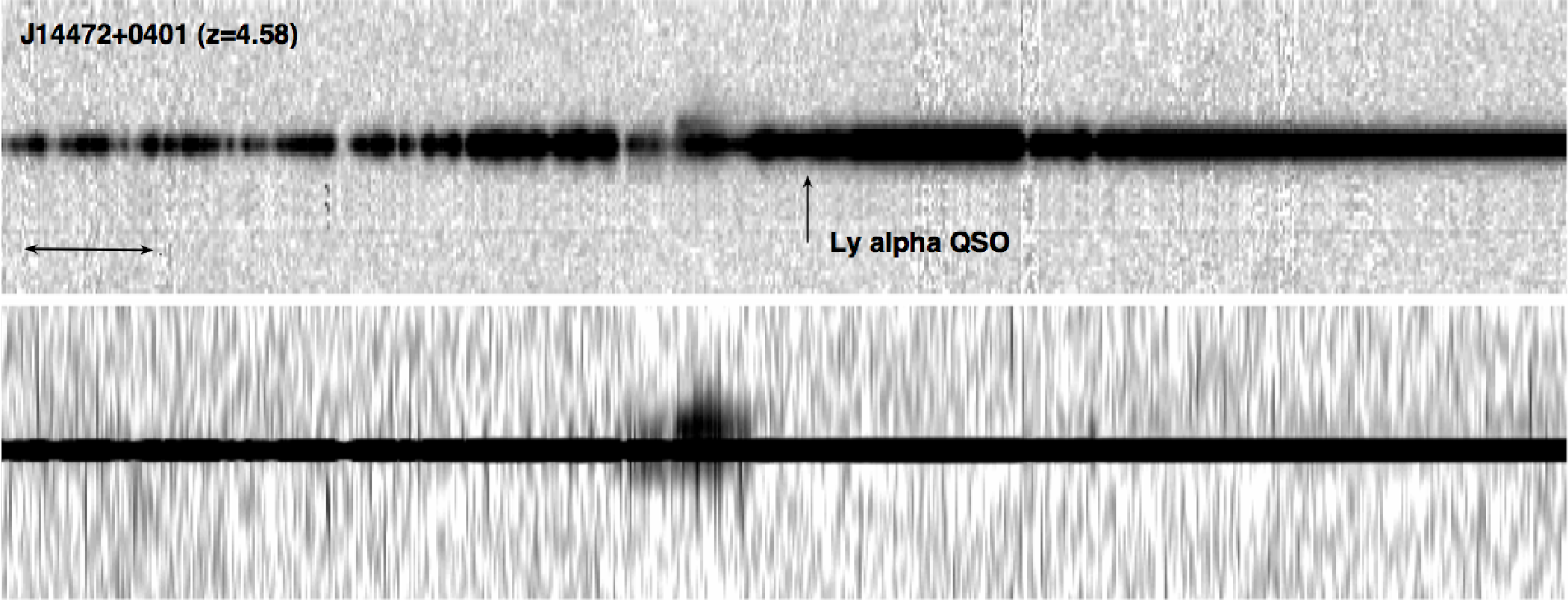
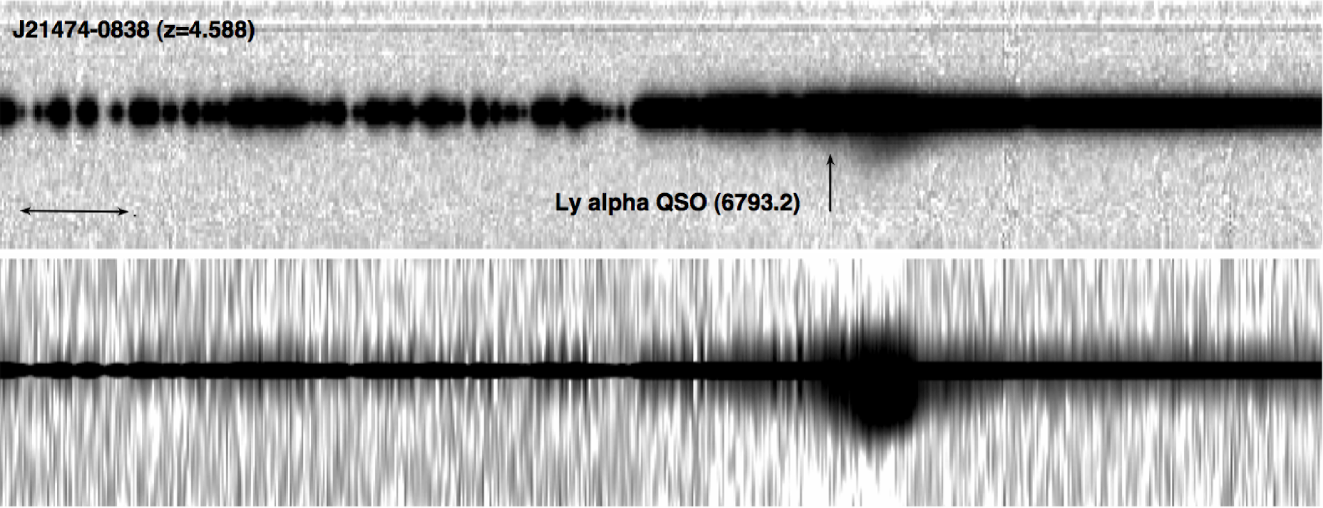
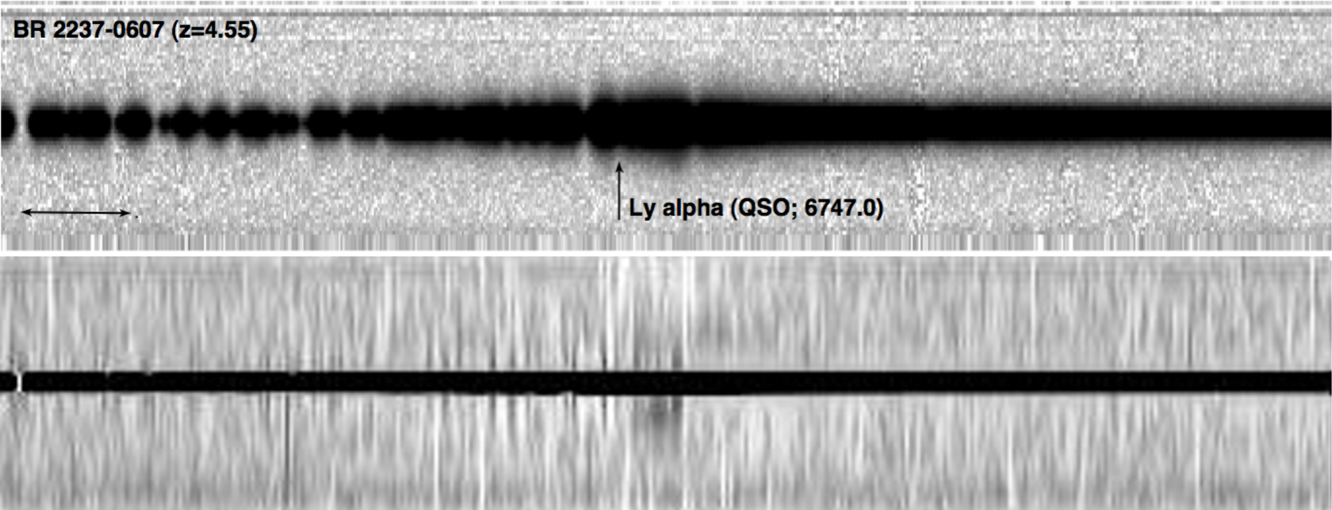
Figure 1: The three combined and sky-subtracted FORS2 spectra along with their spatial deconvolution. The spatial resolution after deconvolution is 0.25″. In each panel, the vertical arrow indicates the position of the Ly$\alpha$  emission line of the quasar, the wavelength of which is indicated. The horizontal double arrow is 50 Å wide. A Ly$\alpha$  envelope is detected in all three quasars. The envelope of SDSS J14472$+$0401 is blueshifted from that of the quasar, while that of SDSS J21474$-$0838 and that of BR 2237$-$0607 are redshifted. The height of the spectra is 16″ in all panels.

2 Deep VLT optical spectroscopy

2.1 Sample and observations

The quasars were selected from the 5th edition of the SDSS catalogue of quasars (Schneider et al., 2007) and from the 12th edition of the Vérons’ catalogue (Véron-Cetty & Véron, 2006). All six objects are listed in Table_QSO of the Vérons’ catalogue with an asterix before their name, which means that they have not been explicitly associated with a radio source in the literature. One of them, BR1033-0327, was explicitly considered as radio-quiet by Kelly et al. (2008). The other objects that were optically detected are probably radio quiet, though statistically a possibility remains that one of them might be radio-loud. The fraction of radio-loud objects in quasars emitting close to the Eddington limit is indeed $\lesssim 5$% (Rafter et al., 2009, Fig. 9); thus, there is at most one chance in three that one of our six quasars is radio-loud.

The observations of the three new targets were carried out in ESO Period 81 (April-September 2008) in service mode with the FORS2 multi-object spectrograph attached to VLT-UT1. The ESO grism G1200R+93 has a resolving power $R=1070$ with a 2″-slit, which ensures that we can catch most of the flux of the Ly$\alpha$  envelope. This grism is used in combination with the GG435+81 order separating filter, leading to the wavelength coverage 6000 Å  $<\lambda<$ 7200 Å. The maximum efficiency of this combination coincides well with the expected wavelength of the redshifted Ly$\alpha$ line, i.e. about 6686 Å.

The multi-slit MXU mode is used, with slits that are long enough (typical length: $\sim 20\arcsec$) to reliably model and subtract the sky emission. Only one scientific target is observable in each field, but the MXU capability is used to observe several stars through identical slits. In this way, a spectral point spread function (PSF) is measured simultaneously with the quasar. This is crucial for the spatial deconvolution of the data to work efficiently (Courbin et al., 2000) and to clearly separate the quasar spectrum from that of the putative envelope.

To properly remove cosmic rays, the total exposure time is split into several shorter exposures. The journal of the actual observations is presented in Table 1.

2.2 Reduction and spatial deconvolution

The data reduction was carried out using the standard IRAF procedures. The individual spectra listed in Table 1 were flat-fielded using dome flats, and wavelength-calibrated in two dimensions in order to correct the sky emission lines for slit curvature. The scale of the reduced data is 0.76 Å  per pixel in the spectral direction and 0.25″  in the spatial direction.

The sky emission was then subtracted from the individual frames by fitting a second order polynomial along the spatial direction. This fit considered only ten pixels on each side of the slit, and the sky at the position of the quasar was interpolated using this fit, both on the quasar and the PSF stars.

The cosmic rays were removed using the L.A.Cosmic algorithm (van Dokkum, 2001). All the frames were visually checked after this process to ensure that no signal was mistakenly removed from the data.

The shape of the spectra along the spectral direction is slightly distorted, i.e., the position of the spectrum changes as a function of wavelength. These distortions are corrected for and the spectra are eventually weighted so that their flux is the same at a reference wavelength, before they are combined to form a deep two-dimensional (2D) spectrum. We show in Fig. 1 the combined spectra of the three new quasars, after binning in both the spatial and the spectral directions. An extended Ly$\alpha$  envelope is already visible in all three objects.

We spatially deconvolved the spectra following the method described in Courbin et al. (2000), which is an adaptation to spectroscopy of the “MCS” image deconvolution algorithm (Magain et al., 1998). The results of this deconvolution are displayed in Fig. 1. The algorithm uses the spatial information contained in the spectrum of several PSF stars in order to sharpen the data in the spatial direction. At the same time, it also decomposes the data into a point-source and an extended-source channel. The output of the deconvolution procedure consists of two individual spectra, one for the quasar and one for its host galaxy (or Ly$\alpha$  envelope), free of any mutual light contamination. It is therefore possible to estimate the luminosity of the Ly$\alpha$  emission “underneath” the quasar. Subsampling of the data is also possible with the MCS algorithm, hence the pixel size in Fig. 1 is half that of the original data, i.e., the new pixel size is 0.125″.

Figure 2: Extracted 1D spectra for the three quasars. In each case, the top panel shows the quasar alone and the bottom panel shows the Ly$\alpha$  envelope alone, after spatial deconvolution of the spectra. The vertical dotted line indicates the position of the un-absorbed Ly$\alpha$  emission line, at the redshift of the quasar (see subsections 3.1 and 2.1). In all cases, the spectrum of the Ly$\alpha$  envelope has been smoothed using a boxcar of 8 Å.

Table 2: Main properties of the Ly$\alpha$  envelopes for all six quasars measured to date (Paper I and this work).

Object	$\lambda$	FWHM	Extent	Integrated flux	$3-\sigma$ detection limit	Surface brightness
	[Å]	[Å]	(″; kpc)	[erg s-1 cm${}^{-2}]$	[erg s-1 cm-2]	[erg s-1 cm-2 ″-2]
SDSS J0939$+$0039	$-$	$-$	$(7;45)$	$-$	$3.9\times 10^{-18}$	$<2.8\times 10^{-19}$
BR 1033$-$0327	$6725.0\pm 0.5$	$50\pm 10$	10;64	$1.4(\pm 0.1)\times 10^{-17}$	$6.7\times 10^{-18}$	$7.2(\pm 0.5)\times 10^{-19}$
SDSS J14472$+$0401	$6756.3\pm 0.5$	$30\pm 3$	6;38	$4.3(\pm 0.7)\times 10^{-18}$	$2.5\times 10^{-18}$	$3.6(\pm 0.6)\times 10^{-19}$
Q 2139$-$4324	$6641.0\pm 0.3$	$-$	$(7;45)$	$-$	$2.2\times 10^{-18}$	$<1.6\times 10^{-19}$
SDSS J21474$-$0838	$6808.2\pm 1.0$	$50\pm 8$	8;51	$3.1(\pm 0.2)\times 10^{-16}$	$3.3\times 10^{-18}$	$1.9(\pm 0.1)\times 10^{-17}$
BR 2237$-$0607	$6773.6\pm 2.0$	$19\pm 2$	4;26	$2.6(\pm 0.8)\times 10^{-18}$	$2.4\times 10^{-18}$	$3.3(\pm 1.0)\times 10^{-19}$

Table 3: Ly$\alpha$  luminosity of the quasars in the BLR, compared with the luminosity of the extended envelopes.

Object	L(BLR)	L(Ly$\alpha$)	Lcorrected(Ly$\alpha$)
	[erg s-1]	[erg s-1]	[erg s-1]
SDSS J0939$+$0039	$4.1(\pm 0.2)\times 10^{44}$	$<7.4\times 10^{41}$	$<2.0\times 10^{42}$
BR 1033$-$0327	$7.2(\pm 0.4)\times 10^{45}$	$2.7(\pm 0.2)\times 10^{42}$	$(1.1\pm 0.1)\times 10^{43}$
SDSS J14472$+$0401	$2.1(\pm 0.1)\times 10^{45}$	$8.6(\pm 1.4)\times 10^{41}$	$(2.0\pm 0.3)\times 10^{42}$
Q 2139$-$4324	$4.6(\pm 0.2)\times 10^{44}$	$<4.1\times 10^{41}$	$<1.1\times 10^{42}$
SDSS J21474$-$0838	$6.8(\pm 0.3)\times 10^{45}$	$6.2(\pm 0.4)\times 10^{43}$	$1.9(\pm 0.1)\times 10^{44}$
BR 2237$-$0607	$1.4(\pm 0.1)\times 10^{46}$	$5.1(\pm 1.6)\times 10^{41}$	$8.0(\pm 2.5)\times 10^{41}$

3 Results

The spectra of the three newly found Ly$\alpha$ envelopes are shown in Fig. 2 together with the spectra of the corresponding quasars (see Fig. 4 of Courbin et al. (2008) for the three other quasars previously observed). The Ly$\alpha$ luminosity of the envelopes, their angular size, and their mean surface brightness are presented in Tables 2 and 3. We integrated the deconvolved spectra in the FORS2 RSPECIAL filter, which is also used to obtain short acquisition images prior to the long spectroscopic exposures. These “spectroscopic” AB magnitudes are given in Table 1. We checked that they are compatible with the simple aperture photometry obtained from the short images.

A Ly$\alpha$ envelope was detected in four objects out of six, which suggests that these envelopes are present in two thirds of the QSOs at $z\sim 4.5$. Our flux limit (integrated over the whole slit and Ly$\alpha$ spectral profile) is indicated in Table 2 and discussed below. The lack of envelope around SDSS J0939$+$0039 and Q 2139$-$4324 may be real, but could also be due to an unfortunate orientation of the slit, if the latter is oriented perpendicular to the long axis of the envelope.

The measurable extent of the envelopes varies (in terms of radius) from $r\sim 20$ kpc for BR 2237$-$0607, to $r\sim 32$ kpc for BR 1033$-$0327, measured from the quasar’s centroid to the noise level in the spatial profiles shown in Fig. 3.

The surface brightness of the Ly$\alpha$  fuzz is unaffected by slit losses, but the total luminosity is. Assuming that the Ly$\alpha$  envelopes are uniform face-on disks with diameters equal to the extents quoted in Table 2, we can estimate the amount of flux missed by using a slit width of 2″. The observed luminosities of the Ly$\alpha$  envelopes for all four quasars are given in Table 3, as well as the luminosities after correction for the slit clipping.

3.1 Detection limit

We now discuss the detection limit. This discussion was not included in paper I, where the detection limit was too optimistic because it was based on the deconvolved images rather than on the original ones. We now redefine this limit for all six objects observed so far (three in Paper I, three in the present work, see Tables 2 and 3). We use the case of BR 2237$-$0607 for this discussion, because it is the target with both the longest exposure time and the faintest envelope if any.

Using spectrophotometric standards, we verified the reliability of the flux calibration by computing the $R_{\mathrm{special}}$ magnitude of the quasar from its observed spectrum, using the $R_{\mathrm{special}}$ filter transmission curve: the obtained magnitude proved to be consistent with that obtained from the imaging observations using the same filter. The maximum intensity of the quasar BR 2237$-$0607 is about $370\,000$ ADU (analogic digital units), for one pixel along the wavelength axis (representing $0.76$ Å), after summation along the spatial axis. Because the corresponding physical flux is $8.41\times 10^{-16}$ erg s^-1 cm^-2 Å^-1 , this extracted pixel (i.e. the pixel of the extracted quasar spectrum) receives a flux of $6.39\times 10^{-16}$ erg s^-1 cm^-2 on its $0.76$ Å width. Conversely, 1 ADU corresponds to $1.73\times 10^{-21}$ erg s^-1 cm^-2 in one pixel. We now consider an extended source rather than a point source: the 8.23 pixels that cover the slit width (considering only one pixel in the spatial direction) correspond to a solid angle of $0.252\arcsec\times 2\arcsec=0.504\arcsec^{2}$ on the sky. Therefore, there are $8.23/0.504=16.33$ pixels within a square arcsecond. Taking into account an observed standard deviation of $\sigma_{i}\sim 40$ ADU (for individual pixels) in the final 2D spectrum (corresponding to a total exposure time of $11\,700$ s), one sees that the standard deviation in the total background intensity, summed over a square arcsecond is (outside the sky emission lines)

$$\sigma(1\arcsec^{2})\approx\sqrt{16.3}\times\sigma_{i}\sim 484\leavevmode\nobreak\ \mathrm{ADU}\sim 8.4\times 10^{-19}\leavevmode\nobreak\ \mathrm{erg\,s}^{-1}\,\mathrm{cm}^{-2}\leavevmode\nobreak\ \mathrm{.}$$ (1)

This is also the error in a signal spread over 1 arcsec², provided that it is small compared to the sky background (which is the case here) and assuming that the latter is sufficiently well-defined to have a negligible error. Therefore, the 3-$\sigma$ minimum signal that can be considered significant after summation across the whole extent of the nebula (spanning $n$ arcsec²) is

$$S(3\sigma)\simeq 12.1\times\sqrt{n}\times\sigma_{i}=484\,\sqrt{n}\leavevmode\nobreak\ \mathrm{ADU}\leavevmode\nobreak\ \mathrm{.}$$ (2)

As a second consistency check, we used the Exposure Time Calculator for FORS2 (ESO version 3.2.7) and were able to confirm the above figures: the flux corresponding to 1 ADU is recovered to within 30% (so the validity of our flux calibration appears to be robust), and the standard deviation in the synthetic 2D spectrum, resulting from a single 11700 s exposure, is only slightly below that of the empirical one ($\sim 30$ ADU instead of $\sim 35-40$ ADU).

In view of the above estimates, it appears that in paper I, we were too optimistic about the detection limit in the case of Q 2139$-$4324: our present calculations imply that the envelope cannot be assumed to have been detected, and only an upper limit can be assigned to its flux.

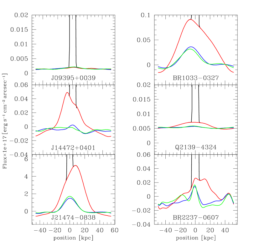
Figure 3: Spatial profiles of the envelopes. The black, quasi-vertical lines show the intensity profile of the quasar, while the red line is the intensity profile of the envelope, integrated across the spectral width of the Ly$\alpha$ line (i.e. an arbitrary range of $20$ Å for objects with no significant envelope, and a $1\times FWHM$ for the other objects). The blue and green lines show the noise, i.e. the profile integrated across wavelength ranges of the same width, but centred $76$ Å bluer, respectively redder than the envelope emission line (except for BR 2237$-$0607, for which the noise was sampled at $\pm 29$ Å from the emission line).

3.2 Comments on individual objects

We now comment on briefly each of the three newly discovered objects.

3.2.1 SDSS J14472$+$0401

The extended emission is blue-shifted with respect to the expected position of the Ly$\alpha$ line of the quasar by $\Delta\lambda=-20\pm 4$ Å, i.e., $\Delta V=-889\pm 180$  km s^-1. The redshift of the quasar may be underestimated, as it is only measured from both the Ly$\alpha$  line itself and the pair of C IV $\lambda 1549$ and C III] $\lambda 1909$ lines, all of which are known to be blueshifted with respect to the actual redshift of the quasar (McIntosh et al., 1999). The Ly$\alpha$  line, on the other hand, is strongly affected by the Ly$\alpha$ forest. If the redshift of the quasar were underestimated, one would expect the surrounding Ly$\alpha$ emission to be redshifted with respect to the expected position of the Ly$\alpha$ line, while we see the reverse. In view of the strong spatial asymmetry of the emitting region (see Fig. 1 and 3), it is possible that the “envelope” is not centred at all on the quasar, but is a blob at some distance away from it. The blue shift may be produced by radiative transfer effects in both a collapsing neutral gas cloud (Dijkstra et al., 2006a, b) and shocks (Neufeld & McKee, 1988).

Interestingly, the nebular emission is matched by a deep absorption feature in the quasar spectrum, at exactly the same wavelength. This is reminiscent of the proximate damped Ly$\alpha$ system (PDLA) discovered by Hennawi et al. (2009) and associated with the quasar SDSS J124020.91+145535.6, except that the Ly$\alpha$ absorption does not seem to be damped in our case. Some non-negligible flux remains at the bottom of the line, and there is no indication of Lorentzian wings in the absorption profile. Nevertheless, the width of this absorption is large, with $FWHM=2100\pm 100$  km s^-1, which is about 50% wider than the emission line of the blob; the lack of damped wings suggests that the FWHM corresponds to the velocity dispersion of the absorbing gas. On the other hand, the emission line seems to have a double structure, which, if taken into account, reaches about the same width as that of the absorption line. Higher dispersion and higher signal-to-noise ratio spectra of this object would allow us to clarify the latter point.

3.2.2 SDSS J21474$-$0838

This is by far the quasar with the brightest Ly$\alpha$ blob in our sample. It is an order of magnitude brighter than the second brightest one, which surrounds the quasar BR 1033$-$0327. As in the latter object, the emission is slightly redward of the expected position of the Ly$\alpha$ line of the quasar, by $\Delta\lambda=+32\pm 4$ Å or $\Delta V=+1400\pm 180$  km s^-1. This is very close to, though slightly larger than, the shift measured in BR 1033$-$0327, and the explanation of it might be the same, i.e. the known blueshift of the Ly$\alpha$, C IV $\lambda 1549$, and C III] $\lambda 1909$ lines. Interestingly, the emission line appears to be slightly asymmetric, with a sharper drop on its red side than the rise on its blue side; a similar asymmetry is seen in the emission line of BR 1033$-$0327. This asymmetry might also be present in SDSS J14472$+$0401, though it is less prominent and possibly due to an absorption feature on the blue side of the emission line.

The positive flux seen on Fig. 2 on both sides of the envelope emission line (and especially on its red side), is probably spurious. There is a bad column on the CCD, running parallel to the quasar spectrum, about 28 pixels away from it (or $7\arcsec$), which may have caused problems with the sky subtraction. The quasar is so bright that a small imperfection in the PSF profile might have produced a pseudo-continuum.

3.2.3 BR 2237$-$0607

This quasar shows the faintest detected Ly$\alpha$ blob in our sample (disregarding the two non-detections), with a luminosity about two times lower than the second faintest blob in our sample (SDSS J14472$+$0401). This is also the most difficult case, since the quasar is the brightest in the sample, so that the contrast between the quasar and the envelope is the largest. This is why it is detected only at the $\sim 3-\sigma$ level, according to the criterion presented in Section 3.1. The emission is strongly redshifted relative to the expected position of the Ly$\alpha$ line of the quasar: $\Delta\lambda=+87\pm 5$ Å or $\Delta V=+3850\pm 220$  km s^-1. Such a considerable shift cannot be explained by absorption, since the Ly$\alpha$ line of the quasar does show significant flux down to at least $6730$ Å  while the nebula emits only between $\sim 6760$ Å and $\sim 6790$ Å. Thus, one has to admit that either the redshift has been underestimated, or the nebula is receding at high velocity from the quasar; it is unlikely that radiative transfer effects could mimick such a fast motion, since one would require a high absorption/emission cross-section in the line profile at these velocities.

3.3 Redshift dependence

The observed surface brightness of the four Ly$\alpha$  envelopes detected in our programme is, on average, fainter by about 1-2 orders of magnitude than for the CJW objects. Our brightest envelope has about the same surface brightness and integrated flux as typical CJW envelopes, while our faintest ones are a hundred times dimmer. This contrast cannot be ascribed exclusively to the different redshift ranges of the two samples. Our sample is at $z_{1}\sim 4.5$, while most of the objects in CJW are at $z_{2}\sim 3.3$, so the flux ratio by redshift dimming alone would be $F(z_{2})/F(z_{1})=(1+z_{2})^{4}/(1+z_{1})^{4}\sim 2.7$, i.e., much smaller than the observed ratio.

Therefore, taken at face value, our sample as a whole suggests that higher-$z$ objects tend to have lower surface brightnesses. The total luminosities of the envelopes in our sample overlap those in CJW: SDSS J21474$-$0838 has a higher Ly$\alpha$ luminosity (when corrected for slit clipping) than all objects in CJW, the envelope of BR 1033$-$0327 has a luminosity close to the average one in the CJW sample, and the two other objects are fainter. Thus, the envelope luminosities in our sample seem to more closely match those of CJW than the surface brightnesses do, but this may be due to our deeper sensitivity. Observations of the CJW envelopes with the same sensitivity as ours would probably reveal that they have faint extensions. Consequently, the envelopes would be found to have higher total estimated luminosities, on the one hand, and a lower average surface brightness, on the other. The spatial extent of the envelopes in our sample ranges from $\sim 26$ kpc to $\sim 64$ kpc, while that of CJW ranges from $\sim 10$ kpc to $\sim 60$ kpc. That explains why the luminosities of our envelopes are often similar to those of CJW, in spite of a much lower surface brightness. The mean size of the envelopes in our sample is indeed $\bar{r}\sim 45$ kpc compared to $\bar{r}\sim 26.4$ kpc in CJW’s sample. This translates into a ratio of 2.9 in area.

The quasar luminosities are slightly larger in CJW’s sample than in ours. The average absolute magnitude $M_{\mathrm{B}}$, as listed in Véron-Cetty & Véron (2006), is $-29.0$ for CJW’s complete sample of seven quasars, while it is $-28.2$ for our sample of six quasars. Since a correlation seems to exist between the luminosity of the quasar and that of the Ly$\alpha$ envelope (see below), such a magnitude difference may explain part of the difference in Ly$\alpha$ envelope luminosities.

A sample of quasars should be observed at $z\sim 3.3$ with the same technique and depth as used at $z\sim 4.5$ in order to settle the question.

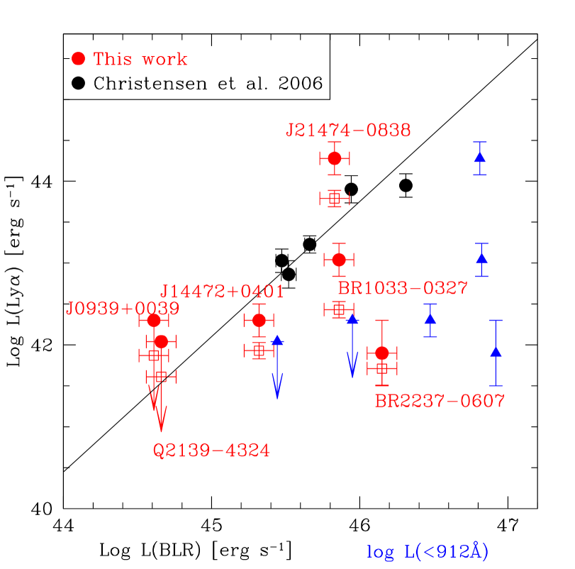
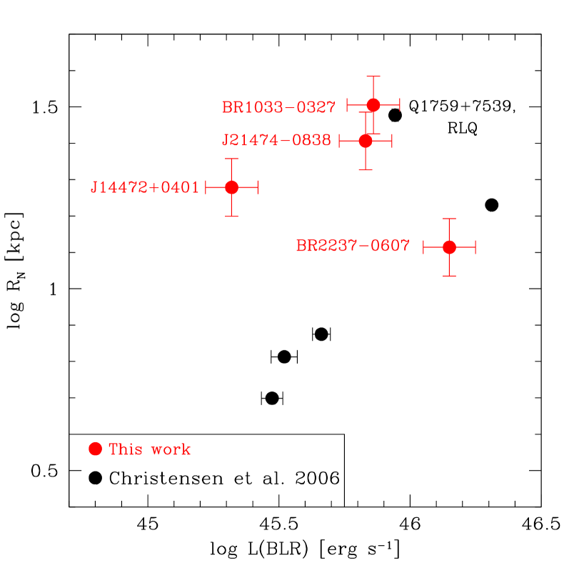
Figure 4: Top: Relation between the total luminosity of the Ly$\alpha$ envelope and that of the quasar in the broad Ly$\alpha$ line. Our measurements (red squares) are compared with CJW (black circles). The open squares represent the direct measurements, while the filled dots are those corrected for slit clipping (see text). The downward arrows show our upper limits for SDSS J0939$+$0039and Q 2139$-$4324, where no Ly$\alpha$  envelope is seen. In computing this limit, we assumed a radius r=23 kpc (i.e., the mean size of the other four objects) and we did not correct for slit-clipping. The black solid line was least squares fitted to the objects of CJW and to our detected envelopes (with correction for slit clipping), except for BR 2237$-$0607. The blue triangles relate the Ly$\alpha$ luminosity (corrected for slit clipping) with the luminosity of the ionizing radiation from the UV continuum of the quasar ($\lambda<912$ Å, see Subsection 3.3). The arrows again show the upper limits to the luminosity of the undetected envelopes. Bottom: The radius of the envelope as a function of $L(BLR)$. Note the tight trend followed by the envelopes of the bright RQQs of CJW. Note also that BR 1033$-$0327  stands above the maximum size of the RQQs of CJW, likely owing to our deeper flux limit.

3.4 Dependence on the luminosity of the quasar

The total flux in the Ly$\alpha$  envelope is shown in Fig. 4 as a function of the quasar luminosity in the broad Ly$\alpha$  line. After correcting for slit-clipping, we find that most points, combined with the ones of CJW, follow the linear relation

$$\log\left[\frac{L(Ly\alpha)}{L({\mathrm{B}LR})}\right]=(0.65\pm 0.53)\times\log[L({\mathrm{B}LR})]-(32.3\pm 24.5)\,\mathrm{,}$$ (3)

suggesting that $L(Ly\alpha)$ varies strongly with $L({\mathrm{B}LR})$. The regression line was determined after excluding BR 2237$-$0607 (the two objects with upper limits to $L(Ly\alpha)$ were not considered). The scatter is $0.39$ dex and the correlation coefficient is $0.874$, leaving no doubt about the statistical significance. Nevertheless, BR 2237$-$0607 remains two orders of magnitude below the linear relation, which seems difficult to explain by slit-clipping effects alone. Since SDSS J0939$+$0039 and Q 2139$-$4324 may also lie well below the regression line, the latter should perhaps be considered as an upper envelope rather than as a real one-to-one relation proper. However, the larger scatter of our points compared to those of CJW around the regression line, may simply reflect our larger uncertainty in L(Ly$\alpha$) due to the slit clipping and unknown shape of the envelope. CJW did not have this problem because they used integral field spectroscopy.

The linear fit implicitly assumes no strong redshift evolution of the luminosity of the envelopes, since it relies on a mix of objects at redshifts $z\sim 3$ and $z\sim 4.5$. Our new observations for the three objects therefore seem to support the trend that brighter quasars also have brighter Ly$\alpha$  envelopes, under the assumption of negligible redshift evolution.

The relation between the size of the envelope and the quasar luminosity is much less clear. CJW find that brighter envelopes tend to be larger, which, combined with the above correlation between envelope and BLR luminosities, implies that brighter quasars should be embedded in larger envelopes. We find no such trend on the basis of our results for our four objects, as shown in Fig. 4 (bottom panel). The marginal trend obtained with the CJW data may be explained by the difficulty in subtracting the quasar light: the brighter the quasar, the wider the envelope has to be in order to be detected unambiguously. Our deeper observations, coupled with a cleaner subtraction of the quasar light, make our results less sensitive to this effect. In addition, the small field of view used in CJW implies that there has been some severe clipping of the envelopes, if they extend much beyond a few arcsecs.

We now examine the possible correlation between the ionizing flux of the quasar and the Ly$\alpha$ flux of the envelope. As in Christensen et al. (2006), we use the template spectrum based on the Sloan Digital Sky Survey (Vanden Berk et al., 2001), completed by the composite Far Ultraviolet Spectroscopic Explorer spectrum of Scott et al. (2004). For simplicity, we adopted the power-law fit $F_{\nu}\propto\nu^{-0.56}$ determined by Scott et al. (2004) to represent the quasar spectrum in the far ultra-violet, from $800$ Å to $912$ Å. We redshifted this composite template spectrum to the observed value of each of our observed targets, and adjusted its intensity so that it matched the observed flux in the range $\sim 1286-1291$ Å in the rest frame ($\sim 7071-7099$ Å at $z=4.5$). Then, we integrated the spectrum between $800$ Å and $912$ Å after having rebinned it to the rest frame, obtaining the ionizing luminosity $L(<912$Å$)$. This luminosity depends of course on the lower integration limit, which is arbitrary. Another choice would have simply changed $L(<912$Å$)$ by a constant factor. Figure 4 (upper panel) shows the Ly$\alpha$ luminosity of the envelope (corrected for slit clipping) as a function of the ionizing luminosity defined above. At first sight, there is no correlation, which tends to confirm the result obtained by Christensen et al. (2006), but at larger redshifts ($z\sim 4.5$) and for a wider range of Ly$\alpha$ luminosities: about 2.3 dex instead of $\sim 1$ dex, taking only the RQQs into account. However, the lack of correlation is essentially due to BR 2237$-$0607, and removing this object would result in a clear trend, similar to the one found using the BLR luminosity instead of $L(<912$Å$)$. Hence, the interpretation of our results depends on the weight given to BR 2237$-$0607: if one fully takes it into account, then there is no correlation and this could be interpreted as an argument against the quasar being the main cause of the Ly$\alpha$ emission of the envelope; conversely, excluding BR 2237$-$0607 as a pathological case restores the correlation and leads to the opposite conclusion. In any case, small number statistics and slit-clipping effects make such a conclusion fragile, as well as the uncertainty inherent to the use of a uniform template spectrum for the quasar.

3.5 Surface brightness and width of the emission line

The FWHM of the Ly$\alpha$ emission line varies by only a factor of $\sim 2.5$ from one object to the other in our sample, but it may be interesting to consider whether it is correlated with e.g. the Ly$\alpha$ luminosity of the nebula. The latter spans a wide range, of about $2.3$ dex. Plotting $\log(FWHM)$ against $\log L$(Ly$\alpha$), we indeed found a rough trend of increasing FWHM (corrected for the intrumental width) with increasing luminosity, although there are four points only, so it is not statistically significant. The correlation coefficient of 0.76 and Student $t$ test of 2.03 leave about a 20% probability of finding the observed correlation by chance alone. Furthermore, the CJW data do not fit the correlation, which confirms that it cannot be real.

Figure 5 presents the average surface brightness of the envelope versus the average FWHM of its Ly$\alpha$ line, for our four objects as well as for the RQQs studied by CJW, for the quiescent halos of radio galaxies of Villar-Martín et al. (2003), and for the RLQs of Heckman et al. (1991a, b). The surface brightnesses taken from the literature were all corrected to a common redshift of $z=4.54$ (the average value of our sample), so that they may be compared. The FWHM values listed in Table 1 of CJW are local values, which do not include the velocity field of the gas; in order to compare with our values, which include a systematic velocity field if any, we estimated “global” FWHM values from the one-dimensional (1D) spectra shown in Fig. 1 of CJW, which are larger since they include the velocity field. The surface brightnesses of the objects of Heckman et al. (1991a) were estimated from their Table 1, by dividing the spectral flux $F_{\mathrm{s}}$ by $1.5\times D_{\mathrm{s}}$ ($1.5\arcsec$ being the width of the slit and $D_{\mathrm{s}}$ the maximum angular extent of the envelope) when the envelope is detected on one side of the quasar only, and by dividing $F_{\mathrm{s}}$ by $3\times D_{\mathrm{s}}$ when the envelope is detected on both sides of the quasar.

It seems that the envelopes of all quasars (whether radio loud or not) and radio galaxies have similar maximum surface brightnesses. Most of our objects lie below the general trend, thanks to our much deeper detection limit, and because not all RQQs are surrounded by bright blobs. On the other hand, the FWHM of the extended Ly$\alpha$ emission spans almost a factor of ten. Surprisingly, the object in our sample that has the highest surface brightness, has a wide FWHM, much wider than those of CJW, and surrounds a RQQ. Our objects with fainter surface brightnesses have, on average, wider emission lines than those of CJW. The reason for this is unclear and this result may be a statistical fluke. Nevertheless, it is interesting to note that the lower left region of the diagram is observationally more accessible than the lower right region, i.e. the detection of low surface brightness envelopes is easier for small FWHMs than for large ones. Therefore, the relative scarcity of objects in this region cannot be the result of an observational bias, and must be real. One can only speculate that the kinematics of these envelopes might be more violent at redshift 4.5 than later, though such a rapid evolution (recalling that the CJW objects are at $z\sim 3.2$) seems doubtful.

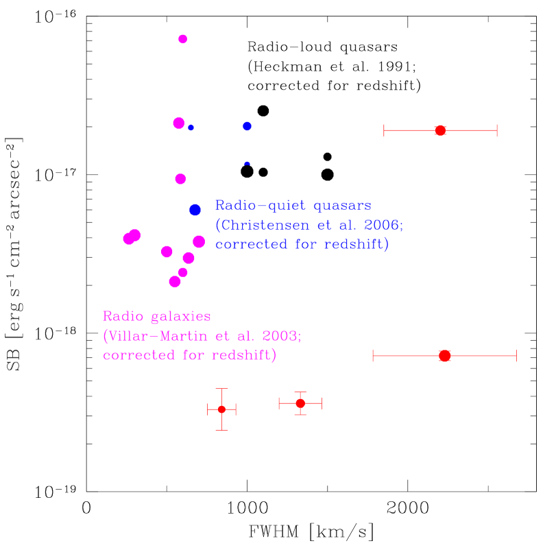
Figure 5: Average surface brightness of the envelope, as a function of the width of the Ly$\alpha$ emission line (expressed in  km s^-1). The red dots represent our results. The surface of the points is proportional to the size of the envelope.

3.6 Upper limit to the flux in the N v doublet

The N v$\lambda 1238.81-1242.80$ Å doublet is not detected in emission, in any of the five envelopes detected here in Ly$\alpha$. It may therefore be interesting to estimate the upper limit to the flux emitted by this doublet, because this may be translated into an upper limit to the metallicity. We performed this estimate in the following very simple way. We adjusted the flux so that the doublet is almost detectable in the 1D spectra of Fig. 2, under the assumptions that: 1) the width of the Ly$\alpha$ line is essentially due to a Maxwellian distribution of the gas velocities, so that the same width can be adopted for each component of the doublet, 2) the two components of the doublet have the same strength, and 3) the intensities of the two components can simply be added. We are aware that our three assumptions are simplistic, especially the second one, which is equivalent to assuming an optically thick gas. The weighted oscillator strength $gf$ of the blue component of the doublet is twice as large as that of the red component (Marsh et al., 1995), so that the ratio of the blue to red component intensities would be two in the optically thin case. The latter case would make the detection easier because the resulting peak would be narrower; conversely, our assumption implies a wider peak, hence a less easy detection, and so appears rather conservative.

The results are summarized in Table 4, which lists respectively the upper limit to the flux possibly emitted in the N v doublet, the flux in the Ly$\alpha$ line, and the ratio of the two. The ratios are not very compelling, since the lowest is $0.14$, meaning that the N v doublet is at least seven times less strong than the Ly$\alpha$ line. One sees that, the narrower the Ly$\alpha$ line, the less compelling the upper limit on the N v doublet, because the flux of the latter is distributed over a wider wavelength range.

Table 4: Upper limits to the flux emitted by the envelope in the N v doublet, compared to the flux emitted in the Ly$\alpha$ line.

Object	Flux(N v)	Flux(Ly$\alpha$)	Flux
	[erg cm-2 s-1]		ratio
BR 1033$-$0327	$\lesssim 2\times 10^{-18}$	$1.4\times 10^{-17}$	$<0.14$
SDSS J14472$+$0401	$\lesssim 1\times 10^{-18}$	$4.3\times 10^{-18}$	$<0.23$
SDSS J21474$-$0838	$\lesssim 5\times 10^{-17}$	$3.1\times 10^{-16}$	$<0.16$
BR 2237$-$0607	$\lesssim 1.3\times 10^{-18}$	$2.6\times 10^{-18}$	$<0.50$

4 Conclusions

We have performed deep slit spectroscopy of six radio-quiet quasars in the redshift interval $4.460\leq z\leq 4.588$ and found extended Ly$\alpha$ emission around four of them. The depth of our detection limit is unprecedented, so we have been able to detect nebulae that are much fainter than in previous surveys.

The main conclusions of this study can be summarized as follows:

• At $z\approx 4.5$, extended Ly$\alpha$ envelopes are found around roughly two-thirds of the quasars.

• The size of the typical envelope is very large (between $\sim 26$ kpc and $\sim 64$ kpc), and does not depend on the Ly$\alpha$ luminosity of the BLR of the quasar.

• The average surface brightness of the envelopes is very low, since it ranges from $\sim 3\times 10^{-19}$ to $2\times 10^{-17}$ erg s^-1 cm^-2 arcsec^-2 . Such low values are due to the large size of the envelopes. Both the large size and the low surface brightness seem difficult to reconcile with a scenario that attributes most of the Ly$\alpha$ luminosity to fluorescence induced by the quasar (Haiman & Rees, 2001).

• The luminosity of the envelopes seems to be correlated with that of the BLR, but this is not an absolute rule, because of the exceptional behaviour of BR 2237$-$0607. Likewise, the envelope luminosity appears to be roughly correlated with the predicted ionizing flux of the quasar, but only when BR 2237$-$0607 is excluded. If confirmed, this trend would resemble that of CJW for RQQs, but over a wider range of luminosities.

• The average FWHM of the extended emission line varies from about $900$  km s^-1 to $2500$  km s^-1 in our sample alone, while it is often smaller in other samples (down to $250$  km s^-1in the radio galaxies of Villar-Martín, 2007).

• The N v$\lambda 1238.81-1242.80$ Å doublet remains undetected in all our objects. The most compelling non-detection occurs in BR 1033$-$0327, where the flux in the doublet is at least seven times lower than in the Ly$\alpha$ line.

Do these results favour the “cold accretion” scenario advocated by Dijkstra & Loeb (2009), or rather the “heating” scenario supported by e.g. Geach et al. (2009)? As discussed above, our results remain ambiguous, because of the unexpected behaviour of BR 2237$-$0607. Arbitrarily discarding this object, the positive trend between the ionizing flux and envelope luminosity might be considered as favouring the heating scenario, but taken at face value our results do not provide enough evidence for either scenario. A larger sample would enable us to settle the issue, because a clear correlation between the AGN UV luminosity and the Ly$\alpha$ luminosity of the envelope is not expected in the cold flow model. In any case, future theoretical works will have to take the observed low surface brightnesses into account. As Haiman & Rees (2001) stress in the last sentence of their paper: “While a detection of Ly$\alpha$ fuzz would provide a direct probe of galaxy formation, nondetections at the level of $10^{-17}$ erg s^-1 cm^-2 arcsec^-2 would already imply strong constraints.” Here, we have provided two non-detections, but at a deeper level (assuming the envelope does extend over at least a few arcsec²), and three detections of envelopes with surface brightnesses significantly lower than $10^{-17}$ erg s^-1 cm^-2 arcsec^-2 . Only one object was found to have a surface brightness of the order of $10^{-17}$ erg s^-1 cm^-2 arcsec^-2 .

A third possibility might be that the detected emission is not actual emission but rather scattering of broad emission-line photons from the quasar. This is suggested by the observed relation $L($Ly$\alpha$$)\propto L(BLR)^{1.65\pm 0.53}$ (Eq. 3), which is compatible to $L($Ly$\alpha$$)\propto L(BLR)^{2}$. The scattered flux is, to zeroth order, proportional to the BLR luminosity times the amount of matter in the envelope; if the latter scales with the bulge mass, which is itself proportional to the supermassive black hole mass, which determines the quasar luminosity, then it is also proportional to the BLR luminosity, indeed implying that $L($Ly$\alpha$$)\propto L(BLR)^{2}$. Photons are then scattered by cool gas on large scales before reaching the observer. Despite the velocity shift between the gas and the quasar redshift (of typically a few hundreds of  km s^-1), there is enough photon flux from the broad quasar emission line (whose width is several thousands of  km s^-1) to produce a nebular fuzz. Admittedly, this argument may prove excessively naive, e.g. because in the cold flow model, the amount of cold gas increases less rapidly than the halo mass (Kereš et al., 2009); the predicted power-law index depends on largely uncertain properties of quasar environments at $z=4.5$, but a more detailed treatment of these issues is beyond the scope of this paper. As for timescales, the nebular size is $<1\times 10^{6}$ light years, hence much shorter than the typical quasar lifetime, which is thought to be of the order of $1\times 10^{7}$ years. That the brighter the broad emission-line emission from the QSO, the stronger the nebular emission, is a result that is consistent with this scattering scenario. The material responsible for the scattering may originate in tidal tails and other debris, associated with the presumably interacting system leading to the onset of quasar activity. This would explain the asymmetry (of the order of $1-2\arcsec$, corresponding to some ten kpc, see Fig. 3) and the extent of the emission (see e.g. Mihos & Hernquist, 1996; Springel, 2000). The observed velocity difference between the peak emission of the QSO and the nebula, $\lesssim 1000$  km s^-1, is rather extreme for a local merger. Nevertheless, the quasar environments at $z\sim 4.5$ may be more extreme than those found at lower redshifts. These quasars may live in proto-cluster like environments with velocity dispersions of order $1000$  km s^-1, which resemble today’s richest clusters. The presence of an additional starburst wind component could contribute to the signal, as well as the cold gas being accreted onto the host galaxy (i.e. the cold flow gas).

Additional spectroscopic measurements at the same redshift would be welcome in order to confirm the correlations found here. However, the crucial data that is badly needed to make progress in understanding these envelopes is narrow-band imaging, which will allow us to obtain much more reliable envelope shapes, extents, and luminosities. The latter are crucial discriminating criteria to identify the mechanism responsible for the envelope emission.