A simple nonlinear equation for structural relaxation in glasses

Abstract

A wide range of glassy and disordered materials exhibit complex, non-exponential, structural relaxation (aging). We propose a simple nonlinear rate equation $\dot{\delta}\!=\!a\left[1\!-\!\exp\left(b\,\delta\right)\right]$, where $\delta$ is the normalized deviation of a macroscopic variable from its equilibrium value, to describe glassy relaxation. Analysis of extensive experimental data shows that this equation quantitatively captures structural relaxation, where $a$ and $b$ are both temperature-, and more importantly, history-dependent parameters. This analysis explicitly demonstrates that structural relaxation cannot be accurately described by a single non-equilibrium variable. Relaxation rates extracted from the data imply the existence of cooperative rearrangements on a super-molecular scale.

Glass-forming materials exhibit rapid increase in relaxation timescales when going through their glass temperature $T_{g}$ AngellReview . When external conditions change abruptly, the observation of the full relaxation to equilibrium becomes exceedingly difficult, except for a narrow range of temperatures near $T_{g}$. The relaxation is characteristically non-exponential and spans several orders of magnitude in time. In many cases, the relaxation is logarithmic. This behavior is paralleled in a broad range of disordered systems: compaction of granular materials Nagel_angle ; Nagel_density , crumpling of thin sheets Nagel_crumpling ; Mokhtar , aging of contact area in dry friction Jay , aging of conductivity in electron glasses Ovadyahu ; Amir and mechanical relaxation of star polymers in gels deGennes ; star_polymer . This apparently wide-spread behavior might suggest a generic origin of slow glassy relaxations (aging).

Glassy relaxation is typically probed by tracking the time evolution of a macroscopic quantity, e.g. the volume or the enthalpy of a sample, in response to an abrupt change in an externally controlled variable, e.g. the temperature. In the latter case, when an initial temperature $T_{0}$ is rapidly changed to $T$, in the vicinity of the glass temperature $T_{g}$, various degrees of freedom of the glass respond differently. The vibrational degrees of freedom quickly equilibrate at the new temperature $T$. The structural degrees of freedom, however, carry long-time “memory” of the original state at $T_{0}$ and fall out-of-equilibrium with $T$. It is the out-of-equilibrium dynamics of the structural degrees of freedom towards a new equilibrium at $T$ that is at the heart of “structural relaxation”.

Structural relaxation is conventionally interpreted in terms of the Tool-Narayanaswamy-Moynihan (TNM) Moynihan , or its equivalent KAHR KAHR , phenomenological 4-parameter models. The main assumption in these models is that during relaxation, a single dynamical variable is sufficient for describing the non-equilibrium state of the glass. In the case of the TNM model this variable is a “fictive temperature”, defined to be a linear function of the probed property, e.g. volume.

However, it is known that these models do not describe experimental data accurately AngellReview , and actually fail to account for thermal history dependence Simon2006 . In addition, while it has been recognized that non-monotonic relaxation (i.e. the Kovacs memory effect Kovacs1963 ) cannot be described by a single non-equilibrium state variable MS-04 ; LEUZZI-09 , some recent works have suggested that this might be possible for monotonic relaxations of the type considered here MS-04 ; BLII-09 ; BL-Kovacs-10 .

In spite of the seemingly universal nature of structural relaxation in glasses, as well as its great scientific and technological importance, a theoretical understanding of it is still missing. In this Letter, we propose a simple, analytically solvable, nonlinear rate equation for describing structural relaxation (aging) in glasses. The proposed equation is shown to quantitatively capture extensive experimental measurements on volume relaxation, yet it explicitly demonstrates the inadequacy of a single non-equilibrium description of glassy relaxation. This analysis allows us to shed light on some basic properties of structural relaxation in these systems, including estimates of activation energy barriers and volumes.

Volume relaxation of glassy materials is usually studied using mercury dilatometry PolymerChemistry . The classical experiments in volume relaxation were performed by Kovacs more than five decades ago Kovacs1963 . These measurements, which in extreme cases reached months, are routinely used and provide a standard testing ground for models. In these so-called down-jump experiments, a glass sample is rapidly quenched from equilibrium at $T_{0}$ to a lower temperature $T$. Measurements begin at $t_{i}$, the characteristic time it takes for the vibrational degrees of freedom to thermalize.

The first question we raise is whether structural relaxation can be properly described by a single non-equilibrium variable model. To address this question, we denote such a variable by $\delta(t)$ and note that a single variable description means that the rate of relaxation is uniquely determined by the instantaneous value of the variable, i.e. $\dot{\delta}(t)\!=\!r[\delta(t)]$, where $r[\cdot]$ is some functional. Therefore, in the framework of such models there exists a function $g(t)$ such that $\delta(t)\!=\!g(t+g^{-1}(\delta_{0}))$, where $\delta_{0}\!=\!\delta(0)$ is the initial condition, and hence a set of measurements which differ only in initial condition could be time-shifted in such a way that all curves would collapse on a single master curve. An example of such a set is shown in Fig. 1(a) with measurements digitized from Kovacs’ original work Kovacs1963 , given in terms of $\delta\!=\!(V-V_{\infty})/V_{\infty}$, the normalized deviation of the volume from its asymptotically stable value $V_{\infty}$. Here the temperature $T\!=\!30^{o}C$ is the same for all measurements, and only the initial state of the system is changed by quenching from different initial temperatures $T_{0}$. In Fig. 1(b), we time-shift each one of the curves such that their initial values would sit on the $60^{o}C\rightarrow 30^{o}C$ curve. The failure of the time-shifted curves to collapse on a master curve implies that using a single non-equilibrium variable (here the deviation of the volume from its equilibrium value) would be inadequate for constructing a predictive model of structural relaxation.

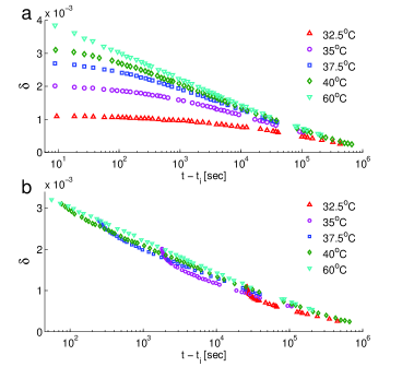
Figure 1: (color online) (a) Down-jumps with a fixed target temperature $T\!=\!30^{o}C$ in PVAc. Data digitized from Fig. 16 in Kovacs1963 . (b) The above measurements time-shifted onto the $60^{o}C\rightarrow 30^{o}C$ curve.

This observation seems to be in line with the common knowledge that glassy relaxation is characterized by a broad spectrum of relaxation times. A fundamental modeling approach would incorporate these various timescales in the time evolution of the probability distribution function of the volume $v$ of mesoscopic material elements $f(v,t)$, as it approaches the stationary equilibrium distribution $f_{T}^{eq}(v)$ at $T$ during structural relaxation. This is a daunting task that has been pursued only in simple models SOLLICH-97 ; 03BBDG . Our goal here is to show that while models that use only the macroscopic volume $V(t)\!=\!N\int_{0}^{\infty}\!vf(v,t)dv$ (where $N$ is the number of elements) cannot be complete, they can still teach us something and might serve as a starting point for constructing an adequate phenomenological model.

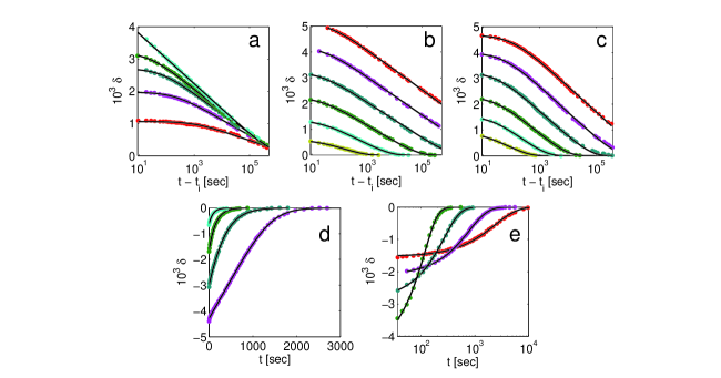
Figure 2: (color online) Fits of Eq. (2) to Kovacs’ data Kovacs1963 . The solid black curves are three-parameter fits. (a) Down-jumps in PVAc with fixed $T\!=\!30^{\circ}C$. See Fig. 1. (b) Down-jumps in PVAc from the same initial condition $T_{0}\!=\!40^{\circ}C$ to $T\!=\!25,...,37.5^{\circ}C$ (top to bottom). (c) Down-jumps in glucose from a fixed initial temperature $T_{0}\!=\!40^{\circ}C$ to $T\!=\!19.8,...,32.5^{\circ}C$ (top to bottom). (d) Up-jumps in PVAc. Note the linear scale. Here $T_{0}\!=\!30,..,37.5^{\circ}C$ (bottom to top) to $T\!=\!40^{\circ}C$. The measurement starts at $t_{i}\!=\!36$ sec. (e) Up-jumps in glucose where $T_{0}\!=\!25^{\circ}C$ is fixed while $T\!=\!30,..,37.4^{\circ}C$ (bottom to top). The measurement starts at $t_{i}\!=\!36$ sec.

There are two basic approaches for understanding logarithmic relaxations. The first approach sees the relaxation as a linear response, i.e. relaxation rates are independent of the state of the system. A logarithmic response can then be obtained by summing over a spectrum of exponential relaxation modes. This approach was suggested in Kovacs1963 , pursued in KimmelUhlmann , and was recently also invoked in the context of electron glasses Amir . Essentially, the evolution of the deviation from equilibrium is assumed to take the form $\delta(t)\!\propto\!\int_{0}^{\infty}\!p(\lambda)\exp(-\lambda\,t)d\lambda$, where $p(\lambda)$ is the distribution of relaxation rates. When $p(\lambda)\!\sim\!\lambda^{-1}$ in a certain range, logarithmic behavior emerges. The second approach, suggested in many contexts (e.g. in Nagel_crumpling ), describes logarithmic relaxation as a result of the dependence of rate on instantaneous state, e.g. slowing-down due to compaction. A nonlinear equation of the form $\dot{\delta}\!\propto\!-\exp(b\,\delta)$ is then proposed to yield $\delta\!\propto\!-\log(t)/b$.

We follow the latter approach and propose to describe structural relaxation by the following equation

$$\dot{\delta}=a\left(1-e^{b\,\delta}\right)\ .$$ (1)

Here $a$ is a basic relaxation rate and $b$ is a constant. The $1$ added in brackets ensures that $\dot{\delta}$ vanishes with $\delta$. Equation (1) admits the analytic solution

$$\delta(t)=-\frac{1}{b}\log\left[1-(1-e^{-b\,\delta_{0}})\,e^{-ab\,t}\right]\,,$$ (2)

where $\delta_{0}$ is the initial condition. For large enough initial amplitudes, for which $\exp(-b\,\delta_{0})\!\ll\!1$, and short times $ab\,t\ll 1$, we have $\delta(t)\!\simeq\!-\log(ab\,t)/b$. The final stage of the relaxation is exponential, $\delta(t)\!\propto\!\exp(-ab\,t)$. For large negative initial amplitudes, for which $\exp(-b\,\delta_{0})\!\gg\!1$, and short times $a\,t\!\ll\!-\delta_{0}$, the relaxation is linear $\delta\simeq\delta_{0}+a\,t$. Again, the final stage of relaxation is exponential, $\delta(t)\!\propto\!-\exp(-ab\,t)$. This marked asymmetry between $\delta>0$ and $\delta<0$ relaxations naturally emerges from the exponential $\delta\!\to\!-\delta$ asymmetry in Eq. (1).

To test the model we present in Fig. 2 fits of Eq. (2) to a significant portion of Kovacs’ original data Kovacs1963 . For each curve the parameters ${\delta_{0},a,b}$ were independently varied. Note, however, that $\delta_{0}$ is essentially determined by the first data point and hence is not a real fitting parameter. Down-jumps in PVAc with fixed target temperature $T$ (panel (a)) and fixed initial condition $T_{0}$ (panel (b)) are satisfactorily captured by Eq. (2). We checked the equation also against data for glucose (panel (c)) which appears in Kovacs1963 . Panels (d-e) show fits to up-jumps - experiments where the initial temperature $T_{0}$ is lower than $T$, making the initial condition $\delta_{0}<0$. Panel (d) is plotted in a linear scale to show the manifestly linear portion of the relaxation. Usually both up-jumps and down-jumps are plotted using a logarithmic time scale to show the asymmetry between the two responses. Here we suggest that this asymmetry can be understood to emerge from the nonlinearity of the response. Additional data were shown to be consistent with Eq. (1) sources .

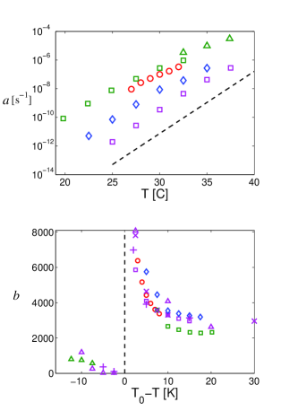
Figure 3: (color online) Variation of the parameters in Eq. (1) with initial temperature $T_{0}$ and target temperature $T$. Legend: ($\boldsymbol{\square}$) PVAc down-jumps from $T_{0}\!=\!40^{\circ}C$ Kovacs1963 ($\boldsymbol{\times}$) PVAc down-jumps to $T\!=\!30^{\circ}C$ Kovacs1963 ($\boldsymbol{\triangle}$) PVAc T-jumps to $T\!=\!40^{\circ}C$ Kovacs1963 ($\boldsymbol{+}$) PVAc T-jumps to $T\!=\!35^{\circ}C$ tau_eff ; Kovacs1963 ($\boldsymbol{\circ}$) PVAc down-jumps from $T_{0}=35^{\circ}C$ SvobodaPVAc ($\boldsymbol{\lozenge}$) PVAc down-jumps from $T_{0}\!=\!40^{\circ}C$ Kovacs1958 ($\boldsymbol{\square}$) Glucose down-jumps from $T_{0}\!=\!40^{\circ}C$ Kovacs1963 ($\boldsymbol{\triangle}$) Glucose up-jumps from $T_{0}\!=\!25^{\circ}C$ Kovacs1963 (a) Variation of relaxation rate $a$ with $T$ for experiments of fixed initial condition. The dashed line is an exponent $e^{T/\tilde{T}}$ with $\tilde{T}=1^{\circ}K$. The error bars are smaller than the symbols. (b) For PVAc and glucose $b$ shows a consistent dependence on jump magnitude $T_{0}\!-\!T$.

Is it a mere curve fitting? Equation (1) provides an excellent description of the data, at a price of independently varying the model parameters for each set of experimental conditions. In addition, we already know that a single variable approach as in Eq. (1) cannot constitute a predictive model. Nevertheless, we argue that the variation of the parameters $a$ and $b$ with experimental condition may be physically meaningful and provide us with physical insight into structural relaxation. Indeed, Fig. 3 shows that $a$ and $b$ do show systematic variations with $T_{0}$ and $T$. Panel (a) shows $a(T)$ for PVAc and glucose under a fixed initial temperature $T_{0}$ (in each experiment, both down and up-jumps). The first observation is that $a(T)$ is a function, i.e. it exhibits a smooth variation with $T$. The same is true for $b(T)$, see panel (b) for measurements with fixed $T_{0}$. In fact, $a$ exhibits a strong exponential dependence on $T$. This is a manifestation of the dramatic slowing down of dynamics associated with the glass transition. The possible origin of this dependence in thermally activated processes will be discussed below.

In the present context, the observation that the structural state of a glass cannot be described by a single non-equilibrium variable implies that $a$ and $b$ should depend on the initial temperature $T_{0}$. Indeed panel (b) demonstrates that $b$ depends on $T_{0}$. Here the parameter $b$ in PVAc and glucose is plotted against the jump size $T_{0}\!-\!T$ for both down-jumps and up-jumps and a wide range of variation of both $T$ and $T_{0}$. This shows that $b$ is in fact a function of both $T$ and $T_{0}$, which strikingly implies that a relaxing glass carries memory of its original state at $T_{0}$ for very long times, sometimes for days! The dependence of $a$ on initial $T_{0}$ (not shown here) is the opposite of that of $b$. In spite of this fact, we have not found any simple connection between the two. We also verified (not shown) that the final exponential relaxation rate, which is controlled by the product $a(T,T_{0})\,b(T,T_{0})$, depends on $T_{0}$ as well.

Another interesting feature of panel (b) is the approximate collapse of all measurements on a single curve as a function of $T_{0}\!-\!T$. This lends support to the view that $b$ has a physical meaning. We also note the apparent discontinuity of $b$ when passing from up-jumps to down-jumps. Discontinuity of this kind in relaxation times is known in the literature as the $\tau_{eff}$-paradox tau_eff . We take it to mean that as the asymptotic volume at $T$ is approached from above (through a down-jump) or from below (through an up-jump), the system explores disparate regions in phase space. This is yet another indication that the volume alone does not tell the whole story about glassy relaxation. This might also be related to the fact that the volume and other thermo-mechanical properties of glasses do not necessarily equilibrate simultaneously (see AngellReview section B.1.8).

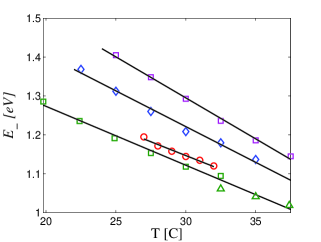
Figure 4: (color online) The volume dependent energy barrier $E_{-}(V_{T})=-k_{B}T\log(a/k_{0})$ for the parameter $a$ in Fig. 3 panel (a). Here $k_{0}=10^{12}$ sec^-1. Solid lines are linear fits.

Equation (1), with its parameters $a$ and $b$, does seem to contain meaningful physical information about the process of structural relaxation. In order to quantify this information, we propose to rationalize the equation using a simple two-state model. A common way to motivate such an equation is to assume that an Arrhenius-like process depends on an observable. In this spirit, let us assume that the volume evolves through activated jumps of volume elements between a contracted “$-$ state” and an expanded “$+$ state”. A rate equation that describes this evolution is

$$\dot{n}=-k_{-}n+k_{+}(1-n)\ ,$$ (3)

where $n$ is the fraction of elements in the $+$ state. A key assumption here is that the activation energies are volume dependent, i.e. $k_{\pm}\propto\exp(-E_{\pm}(n)/k_{B}T)$. $E_{\pm}(n)$ are energy barriers for expansion and contraction. They are assumed to grow with density – it is harder to move in a denser system. Taking into account the fact that $\delta V/V$ is small, of the order of $10^{-3}$, we approximate $n\!\simeq\!n_{T}+\delta n$, where $n_{T}$ is the equilibrium value of $n$ at temperature $T$. By neglecting terms of order $\delta n$, using the equilibrium condition $k_{-}(n_{T})n_{T}\!=\!k_{+}(n_{T})(1-n_{T})$ and writing $\delta_{n}\!=\!\delta n/n_{T}$, we find that

$$\dot{\delta}_{n}=k_{-}(n_{T})\left(e^{A_{+}\delta_{n}}-e^{A_{-}\delta_{n}}\right)\ ,$$ (4)

where $A_{\pm}\!=\!-(n_{T}/k_{B}T)\partial E_{\pm}(n_{T})/\partial n$ are expected to be non-negative, as barriers should become smaller with expansion. Equation (1) then emerges as a special case when $a(T)\!=\!k_{-}(n_{T})$, $A_{+}\!=\!0$ and $b(T)\!=\!A_{-}$.

This model allows us to extract an energy barrier scale from $a=k_{0}\exp(-E_{-}(V_{T})/k_{B}T)$, where $V_{T}$ is the equilibrium volume at $T$. Since $k_{0}$ is a pre-exponential factor, its exact value is not important. We take $k_{0}\!\sim\!10^{12}$ sec^-1, which is the typical scale of molecular vibration. In Fig. 4 we extract values of the energy barrier $E_{-}$ from the experiments summarized in Fig. 3(a). The activation barrier turns out to be on a 1eV scale, which might be indicative of cooperative rearrangements of tens of monomers.

To further test the latter possibility, we estimate the size of rearranging regions by a dimensional argument using the measured derivative $\partial E_{-}(V_{T})/\partial T$. We define a volume scale $v$ as

$$v\sim\kappa V\frac{\partial E_{-}}{\partial V}\sim-\frac{\kappa}{\alpha}\frac{\partial E_{-}}{\partial T}\ ,$$ (5)

where $\kappa\!=\!V^{-1}\partial V/\partial P$ is the isothermal compressibility and $\alpha=V^{-1}\partial V/\partial T$ is the thermal expansion coefficient. Linear regressions shown in Fig. 4 yield $\partial E_{-}/\partial T\!\sim-0.02$ eV/K. Taking for PVAc $\alpha\simeq 7\!\times\!10^{-4}$ K^-1 and $\kappa\!\simeq\!0.42$ GPa^-1 Kovacs1963 we find $v\!\sim\!2$ nm³. A similar estimate for glucose also results in a cubic nanometer scale. These estimates imply that structural rearrangements involve tens of basic units (e.g. monomers in a polymer), which seems consistent with the typical size of dynamical heterogeneities reported in the literature Ediger . Therefore, while the model cannot explain the dependence of the parameters on the initial temperature $T_{0}$, it does seem to be sensitive to the dominant scales of the underlying relaxation processes.

In summary, we proposed a simple mean-field equation to describe structural relaxation in glasses. Our analysis clearly demonstrates that the structural state of a relaxing glass cannot be fully accounted for using a single non-equilibrium variable. In fact, we explicitly showed that a glass may carry information about its thermal history for extremely long timescales. Furthermore, the simple analysis allows the estimation of typical energy and volume scales associated with thermally-activated structural relaxation processes. Theses estimates indicate the existence of cooperative rearrangements on a super-molecular scale.

I.K. is very grateful to R. Svoboda and G.B. McKenna for giving access to data and providing insightful comments. I.K. acknowledges the support of the U.S.–Israel Binational fund (Grant No. 2006288), the James S. McDonnell Fund, and the European Research Council (Grant No. 267256). E.B. acknowledges support from the James S. McDonnell Fund, the Harold Perlman Family Foundation and the William Z. and Eda Bess Novick Young Scientist Fund.

References

- (1) C.A. Angell, K.L. Ngai, G.B. McKenna, P.F. McMillan, and S.W. Martin, J. Appl. Phys. 88, 3113 (2000).
- (2) H.M. Jaeger, C.-h Liu, and S. R. Nagel, Phys. Rev. Lett. 62, 40 (1989).
- (3) J.B. Knight, C.G. Fandrich, C.N. Lau, H.M. Jaeger, and S.R. Nagel, Phys. Rev. E 51 3957 (1995).
- (4) K. Matan, R. B. Williams, T. A. Witten, and S. R. Nagel, Phys. Rev. Lett. 88, 076101 (2002).
- (5) B. Thiria and M. Adda-Bedia, Phys. Rev. Lett. 107, 025506 (2011).
- (6) O. Ben-David, S.M. Rubinstein and J. Fineberg, Nature (London) 463, 76 (2010).
- (7) Z. Ovadyahu and M. Pollak, Phys. Rev. B 68, 184204 (2003).
- (8) A. Amir, Y. Oreg and Y. Imry, Ann. Rev. Cond. Matt. Phys. 2, 235 (2011).
- (9) P.G. de Gennes, J. Phys. France 36, 1199 (1975).
- (10) M. Geoghegan, C.J. Clarke, F. Boué, A. Menelle, T. Russ, and D.G. Bucknall, Macromolecules 32, 5106 (1999).
- (11) C.T. Moynihan et al., Ann. N.Y. Acad. Sci. 279, 15 (1976).
- (12) A.J. Kovacs, J.J. Aklonis, J.M. Hutchinson and A.R. Ramos , J. Polym. Sci. 17, 1097 (1979).
- (13) S.L. Simon, P. Bernazzani, J. Non-Cryst. Solids 352, 4763 (2006).
- (14) A.J. Kovacs, Adv. Polym. Sci. 3, 394 (1963).
- (15) S. Mossa and F. Sciortino, Phys. Rev. Lett. 92, 045504 (2004).
- (16) L. Leuzzi, J. Non-Cryst. Solids 335, 686 (2009).
- (17) E. Bouchbinder and J.S. Langer, Phys. Rev. E 80, 031132 (2009).
- (18) E. Bouchbinder and J.S. Langer, Soft Matter 6, 3065 (2010).
- (19) P.C. Hiemenez and T.P. Lodge Polymer Chemistry 2nd Ed., pp. 474-476 (2007) CRC press.
- (20) P. Sollich, F. Lequeux, P. Hebraud and M. Cates, Phys. Rev. Lett. 78, 2020 (1997).
- (21) E.M. Bertin, J.-P. Bouchaud, J.-M. Drouffe and C. Godrèche, J. Phys. A 36, 10701 (2003).
- (22) R.M. Kimmel and D.R. Uhlmann, J. Appl. Phys. 40, 4254 (1969).
- (23) We tested our equation against data for PVAc from the group of R. Svoboda SvobodaPVAc , from an earlier paper by Kovacs Kovacs1958 and unpublished data from Kovacs’ lab obtained through G.B. McKenna.
- (24) G.B. McKenna et al., Polymer 40, 5183 (1999).
- (25) R. Svoboda, P. Pustková and J. Málek, J. Phys. Chem. Solids 68, 850 (2007).
- (26) J. Málek, R. Svoboda, P. Pustková and P. Čičmanec, J. Non-Cryst. Solids 355, 264 (2009).
- (27) R. Svoboda, P. Pustková and J. Málek, Polymer 49, 3176 (2008).
- (28) A.J. Kovacs, J. Polym. Sci., 30, 131 (1958).
- (29) M.D. Ediger, Ann. Rev. Phys. Chem. 51, 99 (2000).