Progenitor mass constraints for core-collapse supernovae from correlations with host galaxy star formation

Abstract

Using H$\alpha$ emission as a tracer of on-going ($<$16 Myr old) and near-UV emission as a tracer of recent (16-100 Myr old) star formation, we present constraints on the properties of core-collapse supernova progenitors through the association of their explosion sites with star forming regions. Amalgamating previous results with those gained from new data, we present statistics of a large sample of supernovae; 163.5 type II (58 IIP, 13 IIL, 13.5 IIb, 19 IIn and 12 ‘impostors’, plus 48 with no sub-type classification) and 96.5 type Ib/c (39.5 Ib and 52 Ic, plus 5 with no sub-type classification). Using pixel statistics we build distributions of associations of different supernova types with host galaxy star formation. Our main findings and conclusions are:
1) An increasing progenitor mass sequence is observed, implied from an increasing association of supernovae to host galaxy H$\alpha$ emission. This commences with the type Ia showing the weakest association, followed by the type II, then the Ib, with the Ic showing the strongest correlation to star forming regions. Thus our progenitor mass sequence runs Ia-II-Ib-Ic.
2) Overall the type Ibc supernovae are found to occur nearer to bright HII regions than supernovae of type II. This implies that the former have shorter stellar lifetimes thus arising from more massive progenitor stars.
3) While type IIP supernovae do not closely follow the on-going star formation, they accurately trace the recent formation. This implies that their progenitors arise from stars at the low end of the CC SN mass sequence, consistent with direct detections of progenitors in pre-explosion imaging.
4) Similarly the type IIn supernovae trace recent but not the on-going star formation. This implies that, contrary to the general consensus, the majority of these supernovae do not arise from the most massive stars.
Results and suggestive constraints are also presented for the less numerous supernovae of types IIL, IIb, and supernova ‘impostors’. Finally we present analysis of possible biases in the data, the results of which argue strongly against any selection effects that could explain the relative excess of type Ibc supernovae within bright HII regions. Thus intrinsic progenitor differences in the sense of the mass sequence we propose remain the most plausible explanation of our findings.

1 Introduction

Core-collapse (CC) supernovae (SNe) are the explosive fate of massive ($>$8-10${\rm\ M}_{\odot}$) stars. This occurs after successive stages of nuclear fusion lead to the formation of a degenerate iron core. Nuclear fusion is then energetically unfavorable and continued energy losses accelerate the collapse of the core. The bounce of this collapse once nuclear densities are reached, and its subsequent interaction with still infalling material aided by copious neutrino fluxes, is thought to produce a shock wave that expels the star’s envelope generating the transients we observe (see Mezzacappa 2005, for a review of the latter stages of stellar evolution that lead to core collapse and SN).
The immense temperatures, densities and energies reached during the explosive CC process lead to CC SNe playing a huge role in defining the evolution of their environments, and hence the Universe. They are responsible for a significant fraction of heavy elements produced, and their energetics impact into their local environments, driving galaxy evolution and possibly triggering further star formation (SF).
However, the community is still far from agreement on which types of progenitors give rise to the rich diversity in transient light curves and spectra we observe. Mapping the paths between progenitor characteristics and transient phenomena has become a key goal of SN science that is rapidly increasing our understanding of stellar evolution and the role parameters such as metallicity, rotation and binarity play in the final stages of the lives of massive stars.

1.1 CC SN types

SNe were initially separated into types I and II through the absence or presence of hydrogen in their spectra (Minkowski, 1941). While all type II events are thought to be produced through the CC mechanism, in addition the types Ib and Ic of the non-hydrogen class are also believed to occur through CC. Hence when speaking on the overall CC family we are discussing those SNe classified as II, Ib or Ic. SNe types Ib and Ic (throughout the rest of the paper when referring to ‘SNIbc’ we are discussing the group of all those SNe that are classified in the literature as ‘Ib’, ‘Ic’ or ‘Ib/c’) lack strong silicon absorption seen in SNe type Ia (SNIa; thermonuclear events), while the two are distinguished by the presence (in the former) and absence (in the latter) of helium in their spectra (see Filippenko 1997 for a review of SN spectral classifications). SNe type II (SNII henceforth) can be further split into various sub-types. SNIIP and SNIIL are differentiated by their light-curve shapes, with the former showing a plateau and the latter a linear decline (Barbon et al., 1979). SNIIn show narrow emission features in their spectra (Schlegel, 1990), indicative of interaction with pre-existing, slow-moving circumstellar material (CSM, Chugai & Danziger 1994). SNIIb are transitional objects as at early times they show hydrogen features, while later this hydrogen disappears and hence their spectra appear similar to SNIb (Filippenko et al., 1993). Finally, there is a group of objects known as ‘SN impostors’. These are transient objects which when discovered appear to be similar to SNe (i.e. events that are the end-points of a star’s evolution), but are likely to be non-terminal, and hence possibly recurring, explosions from massive stars (e.g. van Dyk et al. 2000; Maund et al. 2006, although see Kochanek et al. 2012).
While the exact reasons for differences in light-curves and spectra are unknown, they are likely to be the product of differences in initial progenitor characteristics (mass, metallicity, binarity and rotation) which affect the stellar evolution of the star prior to SN. Effectively, these differences change the final structure of the star and its surroundings prior to explosion and hence produce the diversity of transients we observe. The main parameter affecting the nature and evolution of the light we detect from a SN would appear to be the amount of stellar envelope that is left at the epoch of explosion, with the SNIIP retaining the most and the SNIc retaining the least. This outer envelope can be lost through stellar winds, or through mass transfer in a binary system. These processes are then dependent on 4 main progenitor characteristics: initial mass, metallicity, stellar rotation and the presence/absence of a close binary companion. Given the likely strong correlation between pre-SN mass loss and resultant SN type it has been argued (see e.g. Chevalier 2006) that the CC classification scheme can be placed in a sequence of increasing pre-SN mass-loss such as follows:

SNIIP $\rightarrow$ IIL $\rightarrow$ IIb $\rightarrow$ IIn $\rightarrow$ Ib $\rightarrow$ Ic

Our understanding of the accuracy of this picture and how it relates to progenitor mass or other characteristics is far from complete. However, it is a useful starting point and we will refer back to this sequence when later discussing our results which imply differences in progenitor lifetimes and hence initial masses.

1.2 CC SN progenitor studies

The most direct evidence on progenitor properties is gained from finding pre-SN stars on pre-explosion images after a nearby SN is discovered. This has had success in a number of cases (see e.g. Elias-Rosa et al. 2011 and Maund et al. 2011 for recent examples, and Smartt 2009 for a review on the subject), and long-term we are likely to gain the best insights into progenitor properties through this avenue. However, while the direct detection approach can give important information on single events, the need for very nearby objects limits the statistics gained from these studies. Therefore it is useful to explore other avenues to further our understanding of SN progenitors from a statistical viewpoint.
An easy to measure parameter of a single SN is the host galaxy within which it occurs. This separation of events by galaxy type was one of the initial reasons for the separation into CC (requiring a massive star) and thermonuclear (arising from a WD system) events, through the absence of the former in ellipticals (see e.g. van den Bergh et al. 2005) where the stellar population is almost exclusively dominated by evolved stars. More detailed studies have investigated how the relative SN rates change with, e.g. luminosities of host galaxies (e.g. Prantzos & Boissier 2003; Boissier & Prantzos 2009; Arcavi et al. 2010), to infer metallicity trends, or have obtained ‘direct’ host galaxy metallicity measurements through spectroscopic observations (Prieto et al., 2008). These valuable studies allow the inclusion of large numbers of SNe enabling statistically significant trends to be observed. However, in a typical star forming galaxy there are many distinct stellar populations, each with its own characteristic age, metallicity and possibly binary fraction. Therefore, to infer differences in progenitor properties a number of assumptions have to be made. For CC SNe, which have sufficiently short delay-times (period between epoch of SF and observed transient) that the position at which an event is found is close to its birth site, it is arguably more important to attempt to characterise the exact environment within host galaxies where SNe are found, in order to pursue progenitor studies.
This is the approach we proceed with in the current study; investigating correlations of SN type with the characteristics of their environments within host galaxies in order to constrain progenitor properties.

1.2.1 Core-collapse SN environments

The distribution of massive stars in galaxies is traced by the presence of HII regions and OB associations. Therefore, one can analyse the distribution of SNe within host galaxies and compare these with those of massive stars in order to attempt to constrain the former’s progenitors. After initial studies by Richter & Rosa (1984) and Huang (1987), van Dyk (1992) was the first to attempt to separate CC SNe into SNII and SNIbc with respect to host environments. He found no statistical difference between the association of the two with HII regions, albeit with low statistics. Further studies were achieved by Bartunov et al. (1994) and van Dyk et al. (1996) who again concluded that the degrees of association of the two types were similar and hence suggested that both types arose from similar mass progenitors (later a detailed discussion will be presented on how these associations can be interpreted). These studies measured distances to nearby HII regions to gauge associations with massive star populations. While this approach can give useful information on individual SNe associations, the irregular nature and large range of intrinsic sizes/luminosities of HII regions mean that objectively applying this technique can be difficult.
More recently, a pixel statistics technique has been developed (James & Anderson, 2006; Fruchter et al., 2006) which allows one to investigate SN distributions in a more systematic way. Kelly et al. (2008) used this technique to investigate the association of SNe and long-duration Gamma Ray Bursts (LGRBs) with host $g$-band light. They found that while the SNIa, SNII and SNIb followed the $g$-band distribution, the SNIc and LGRBs were found to occur more frequently on peaks of the flux, and hence they concluded that both type of events arose from similarly massive progenitors. Raskin et al. (2008) compared these distributions with predicted characteristic stellar ages from analytical models of star-forming galaxies, and derived mass limits for CC SNe, concluding that SNIc arise from progenitors with masses higher than 25${\rm\ M}_{\odot}$. Leloudas et al. (2010) looked specifically at the distribution of SNIbc locations and compared them with those of Wolf-Rayet (WR) stars in nearby galaxies, claiming that SNIbc were consistent with being produced by these stars.
In addition to investigating correlations of SNe with certain stellar populations, one can look at radial distributions of events and attempt to infer progenitor properties, by comparing these to parameters such as metallicity gradients within galaxies. Following Bartunov et al. (1992), van den Bergh (1997) found a suggestion that SNIbc are more centrally concentrated within host galaxies than SNII, a result which has been confirmed with increased statistics by Tsvetkov et al. (2004), Hakobyan (2008), Anderson & James (2009) and Boissier & Prantzos (2009). These differences have generally been ascribed to a metallicity dependence in producing additional SNIbc at the expense of SNII in the centres of galaxies which are believed to have enhanced (compared to the outer disk regions) metal abundances (see Henry & Worthey 1999). These trends are expected on theoretical grounds as at higher metallicity progenitor stars have higher mass-loss rates through radiatively driven winds (see e.g. Puls et al. 1996; Kudritzki & Puls 2000; Mokiem et al. 2007) and hence it is easier for a star to lose its outer envelopes and explode as a SNIbc. However, this simple interpretation has been questioned by recent work separating galaxies by the presence of interaction or disturbance (Habergham et al., 2010). This analysis found that the centralisation is much more apparent in disturbed galaxies. Given that these disturbed galaxies are likely to have much shallower (if any) metallicity gradients (Kewley et al., 2010) it was concluded that there was an IMF effect at play. A detailed follow-up paper addressing these issues is being prepared (Habergham et al. in preparation).
A more direct way to measure environment metallicities is to obtain spectra of the immediate environments of SNe and derive gas-phase metallicities from emission line diagnostics. This approach was first achieved by Modjaz et al. (2008) who looked specifically at the environments of GRBs and the broad-line SNIc which are associated with GRBs. Subsequent works have searched for differences between the CC types. Modjaz (2011) and Leloudas et al. (2011) investigated differences between SNIb and SNIc but came to different conclusions on whether there was any clear metallicity difference, while Anderson et al. (2010) included a sample of SNII in addition to SNIbc and found that the SNIbc show only a small, barely significant offset to higher metallicity than SNII, while also finding little difference between the SNIb and SNIc. These studies are continuing, with care being taken to include SNe from all types of host galaxy in order to remove possible biases (see Modjaz 2011, for a recent review of these results).
Most recently Kelly & Kirshner (2011) have combined many of the above techniques by using images and spectra from the Sloan Digital Sky Survey (SDSS) to investigate environmental colours and host galaxy properties of SNe of different types, and have used these observations to infer differences in progenitor properties.
Our first contribution to this growing field was published in James & Anderson (2006). Here we introduced a pixel statistic (which is the main analysis tool used for the current investigation), and used this together with other analyses to investigate how SNe are associated with SF within their host galaxies, as traced by H$\alpha$ emission. The CC SN pixel statistics analysis of this work was then updated with an increased sample size of 160 CC SNe in Anderson & James (2008) (AJ08 hereafter). In the current paper we repeat this analysis but with significantly larger samples. The current analysis is achieved on a sample of 260 CC SNe. After a thorough search of the literature this sample can be broken down to 58 SNIIP, 13 IIL, 13.5 IIb (one SN, 2010P is classified as IIb/Ib in the literature and is therefore added at half weighting to both distributions), 19 IIn, 12 SN ‘impostors’ and 48 SNe that only have ‘II’ classification, plus 39.5 SNIb, 52 Ic and 5 SNe which only have ‘Ib/c’ classification in the literature. We analyse the association of all these SNe to SF within their host galaxies and use these results to infer properties of their respective progenitors.
The rest of the paper is arranged as follows. Next we summarise the data used and reduction processes applied, followed by a summary of our pixel statistics technique in section 3. Then we present our results in section 4, followed by a discussion of their implications for the properties of CC SN progenitors in section 5. Finally we list our conclusions in section 6.

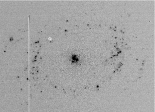
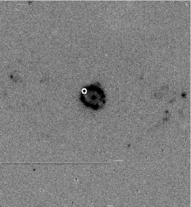
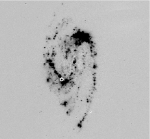
Figure 1: Examples of negative continuum-subtracted H$\alpha$ images used in our analysis. In all images the location of the SN is marked by the white circle and north is up with east to the left. The left hand panel shows an ESO 2.2m image of NGC 1433, the host galaxy of the type IIP SN1985P. Here the ‘NCR’ pixel value is 0.000. In the centre panel we show an LT image of NGC 1343, the host galaxy of the type Ic SN2008dv. The analysis of this image gives an ‘NCR’ value of 0.802 for the SN. Finally in the right hand panel we show an INT image of NGC 3627, the host galaxy of the type IIL SN2009hd. The ‘NCR’ value for SN2009hd is 0.398.

2 Data

The data used for this study have been assembled over a number of years from range of projects, many of which were not originally focused on SN environment studies. Therefore our sample is quite heterogenous in terms of SN and galaxy selection. While this means that the host galaxies analysed and the relative numbers of SNe contain significant biases, what we should have is a sample of SNe and their host galaxies which are a random selection of the, to-date, ‘observed’ local SNe, the only proviso being that we have favoured SNe with sub-type classification. The data now discussed are an amalgamation of ‘new’ data with that presented in AJ08.
All SNe within the sample have host galaxies with recession velocities less than 10000 kms^-1 (the majority have recession velocities less than 6000 kms^-1), with a median velocity of 1874 kms^-1. We exclude all SNe that occur within highly inclined disk galaxies with axis ratios higher than 4:1, in order to reduce the occurrence of chance superpositions of SNe onto foreground/background stellar populations. Data that were obtained specifically for this project were chosen where SNe sub-type information was available in the literature. This introduces the bias that many of the SNII with sub-type classification fall within galaxies at lower redshift than the SNIb/c population. We later discuss the origin of this bias and investigate whether this has any effect on our results and conclusions. SN types were originally taken from the Asiago catalogue, but the literature was extensively searched for further information, and in some cases SN types were changed (these instances are listed in table A1). We do not include any ‘02cx-like’ objects (see e.g. Jha et al. 2006; Foley et al. 2009) due to the unclear nature of their origin, while we also exclude ‘Ca-rich’ objects (see e.g. Filippenko et al. 2003; Perets et al. 2010, 2011), again due a possible distinct progenitor population. As we are interested in the stellar population within the environment of each SN we do not wish to detect any remaining emission from the SNe themselves. Therefore we introduce a criterion that host galaxy imaging must have been taken at least 1 year post SN discovery date for SNIbc and 1.5 years for SNII (which for the case of SNIIP, the most dominant type, are likely to have longer lasting light curves). This criterion is difficult to apply to SNIIn. These SNe sometimes show very long term (sometimes on the order of decades; e.g. Bauer et al. 2008) interaction, which can manifest as H$\alpha$ emission, and thus could easily mimic environment HII regions where none actually exist. However, given our results presented in section 4.1 of a non-association of SNIIn to SF as traced by H$\alpha$ emission, any ‘false’ associations, were they removed, would only increase the significance of our results. Therefore we apply the same criterion to these SNe as to other SNII.
Following AJ08 some of the data initially included in this analysis have now either been removed or a SN type classification has been changed. Here we list these changes:
SN 1996ae: SN removed from analysis due to axis ratio of host
SN 2002gd: SN removed from analysis due to axis ratio of host
SN 2002bu: type classification changed to ‘impostor’ following Smith et al. (2011)
SN 2004gt: type classification changed to SNIc following reclassification in Asiago catalogue
SN 2006jc: type classification changed to SNIb following reclassification in Asiago catalogue
SN 2001co: SN removed from analysis as classified as ‘Ca-rich’ object (Aazami & Li, 2001)
SN 2003H: SN removed from analysis as classified as ‘Ca-rich’ object (Graham et al., 2003)
We note that none of these changes would alter the overall results and conclusions presented in AJ08.
For the subsequent analysis we will use both H$\alpha$ and near-UV emission as tracers of SF of different characteristic ages. H$\alpha$ emission observed in SF galaxies is produced by the recombination of hydrogen ionised by massive stars. This emission is generally observed as bright HII regions within galaxies that are thought to be consistent with stellar ages of less than 16 Myr (Gogarten et al., 2009). Near-UV emission (defined here as that detected by the Galaxy Evolution Explorer; $GALEX$, near-UV pass-band which is centered at $\lambda$ = 2316Å) is that produced by hot massive stars (but including less massive stars than those needed to produce H$\alpha$ emission) and is thought to trace episodes of SF on timescales between 16 and 100 Myr (Gogarten et al., 2009). Hence, H$\alpha$ emission is tracing SF on shorter timescales than that traced by near-UV emission. Therefore we choose to define SF as traced by H$\alpha$ as on-going, while that seen at near-UV wavelengths as recent SF. This nomenclature will be used for the remainder of the paper.

2.1 New H$\alpha$ imaging

2.1.1 MPG/ESO 2.2m data

H$\alpha$ narrow- and $R$-broad band imaging (used for continuum subtraction) were obtained for 43 CC SNe host galaxies with the Wide Field Imager (WFI) mounted on the 2.2m MPG/ESO 2.2m telescope (referred to as ‘ESO’ in table A1) at La Silla, Chile, giving images with pixel sizes of 0.238 arcseconds per pixel. Data were obtained using the narrow-band ‘Halpha/7’ and ‘665/12’ filters, and exposure times of $\sim$900s (split into 3x300s to remove cosmic rays by median stacking) for the narrow band filters and 300s in $R$-band were generally used. Data were reduced in a standard way, which will be summarised for all instruments below.
In Fig. 1 we show examples of 3 continuum-subtracted H$\alpha$ images of SN host galaxies used in the current analysis.

2.1.2 Additional LT data

28 ‘new’ CC SNe were found to have occurred either in old data (i.e. SNe that were discovered in data presented in AJ08, Anderson & James 2009, but after their publication), or new data specifically obtained for this project, with RATCam mounted on the Liverpool Telescope (LT) at La Palma, the Canary Islands. These data were obtained using the narrow H$\alpha$ filter and broad $r^{\prime}$-band filter (used for continuum subtraction), and data were binned 2x2 giving pixel scales of 0.276 arcseconds per pixel. Images were obtained with exposure times of $\sim$900s (split into 3x300s to remove cosmic rays by median stacking) for the narrow band filter and 300s in the $r^{\prime}$-band. These data were automatically processed through the LT pipeline giving bias-subtracted and flat field-normalisation images that were then processed as outlined below before analysis.

2.1.3 Additional JKT data

H$\alpha$ and $R$-band galaxy imaging were recovered from previous projects of one of the authors (PAJ). These were generally projects to investigate the SF properties of nearby galaxies. The catalogues were searched and 14 ‘new’ CC SNe were found to have occurred within galaxies imaged by the Jacobus Kapteyn Telescope (JKT), on La Palma, the Canary Islands. These images have a pixel scale of 0.33 arcseconds per pixel. Data were obtained through a range of projects and hence different filters and exposure times were used for different galaxies. Details of examples of those data obtained for the H$\alpha$GS (H$\alpha$ galaxy survey), and their reduction, can be found in James et al. (2004). Data were generally obtained with exposure times giving similar H$\alpha$ sensitivity as other data presently analysed.

2.1.4 Additional INT data

Data were also recovered from other projects that were taken with the Wide Field Camera (WFC), mounted on the Isaac Newton Telescope, at La Palma, the Canary Islands. Either new data were found, or additional SNe had occurred within data presented previously, in 11 cases. Again these data were obtained in a similar fashion to that above, and were reduced in a similar way. The WFC pixel size is 0.333 arcseconds per pixel.

2.1.5 H$\alpha$ data reduction

All H$\alpha$ and $R$- (or $r^{\prime}$-) band data were reduced in a standard manner, which has been discussed in detail in James et al. (2004) and also in previous papers in this series (AJ08, Anderson & James 2009). The narrow- and broad-band data were processed through the usual stages of bias-subtraction and flat-field normalisation before H$\alpha$ images were continuum-subtracted using the broad-band exposures, using routines in IRAF and Starlink. The continuum subtraction was achieved by first aligning and scaling the narrow- to broad-band images, then stars within the field were used to estimate a continuum scaling flux factor between the two exposures. After using this factor to normalise the broad-band images to that of H$\alpha$, we used the former to remove the contribution of the continuum to the narrow-band images, leaving only the flux produced by H$\alpha$ (and [N ii]) line emission. In general this process works well, however in some cases individual images need to be re-processed through an iteration in order to obtain a satisfactory continuum subtraction.
Bright foreground stars often leave residuals after the subtraction process. These residuals are removed through ‘patching’ of the affected image regions (pixel values are changed to average values of those just outside the affected region). When the affected region covers a large portion of the galaxy, or is extremely close to the SN position we remove these cases from our statistics due to the uncertainties this may cause. Finally all images are processed to leave a mean sky value of zero.
In order to accurately derive the position where each SN exploded within its host galaxy, we require accurate (sub-arcsecond) astrometry. Therefore we determined our own astrometric solutions for all images within the sample using comparison of stars with known sky coordinates from second generation Palomar Sky Survey XDSS images downloaded from the Canadian Astronomy Data Centre website, and used the $Starlink$ routine ASTROM to calibrate images. Finally, all the above images are binned 3x3 to decrease the effects of uncertainty in SN coordinates on our analysis. Hence all images are analysed with effective pixel sizes of $\sim$1 arcsecond. The median recession velocity of the sample of host galaxies is 1874 kms^-1. Therefore, at this distance we are probing physical sizes of around 130 pc. At the distance of the closest galaxy (NGC 6946) we probe distances of $\sim$40 pc, while for the most distant galaxy (UGC 10415), the corresponding resolution is much coarser, $\sim$650 pc. Hence, in most cases we do not probe individual HII regions, but larger SF complexes within galaxies. Later in the paper we will show that splitting the sample by host galaxy distance makes little difference to the results obtained, hence we are confident in our analysis technique with respect to this issue.

2.2 GALEX data

As we will show below, many CC SNe do not follow the on-going SF as traced by H$\alpha$ emission. Therefore, we decided to probe the association of certain SN types with SF of longer characteristic lifetimes. To do this we chose to use GALEX near-UV images, and as outlined above we define that the emission detected in these images is that from recent SF, i.e. that on timescales between 16 and 100 Myr (Gogarten et al., 2009). We chose to use near-UV images in place of GALEX far-UV images for two reasons. 1) In terms of the ages of SF traced by the two, the near-UV emission gives a longer time baseline compared to that traced by H$\alpha$ emission, and hence we can hope to see larger differences in the association of the different SNe to the different emission. 2) There are fewer detections at far-UV wavelengths and therefore using the far-UV images would lead to larger uncertainties where no emission is detected.
For all those SNe where we require UV imaging, we use the $GALEX$ search form to download host galaxy images. $GALEX$ has obtained data for a range of projects from an all sky survey (AIS), to individual time requests of smaller samples (details of the surveys achieved can be found in Morrissey et al. 2007). Hence for some galaxies within our sample there is a range of images to choose from. For each galaxy we use the deepest images available. These near-UV images display the emission at wavelengths between 1770 and 2730 Å and have pixel sizes of 1.5 arcsecond per pixel. Hence, these images probe similar physical sizes to those taken with ground-based optical detectors as outlined above.

3 Pixel statistics analysis

The pixel statistic used throughout this paper has been used and described in detail in previous works. Here, we briefly summarise the formulation and use of this statistic, but we refer the reader to those previous papers (James & Anderson 2006, AJ08) for more in depth discussion of the technique and its associated errors. In latter sections we delve deeper into some un-addressed issues that may be important for the interpretation of the use of this statistic on our SN and galaxy samples.
Our ‘NCR’ (a shortened acronym of the ‘Normalised Cumulative Rank pixel function’, first presented in James & Anderson 2006) statistic gives, for each individual SN, a value between 0 and 1 which corresponds to the amount of emission within the pixel of a SN, in relation to that of the whole host galaxy. It is formed in the following way, from continuum-subtracted H$\alpha$ images (plus GALEX near-UV in the present paper). First, the images are trimmed so that we only include emission of the galaxy and the SN position. This helps to avoid large fluctuations in the sky background and/or bright foreground stars in the vicinity of the host, which sometimes prove difficult to remove. The pixels from each image are then ranked in terms of increasing count; i.e. from the most negative sky value, up to highest count from the pixel containing the most flux within the frame. We then form the cumulative distribution of this ranked pixel count, and finally normalise this to the total flux summed over all pixels. We set all negative values in this cumulative distribution to 0. Hence, NCR values of 0 correspond to the SN falling on zero emission or sky values, while a value of 1 means that the SN falls on the brightest pixel of the entire image. We proceed with this analysis for all SNe within the sample (using the same technique for both H$\alpha$ and near-UV images, where they are included), building distributions for the different CC SN types. If we assume that the SF pixel count scales by number of stars being formed (with near-UV emission simply tracing stars down to lower masses), then if a SN population accurately follows the stars being formed and mapped by that particular SF tracer, we expect that the overall NCR distribution for that SN type to be flat and to have a mean value of 0.5. We use this as a starting point for interpreting our results on the different SN types, and investigate differences in the association of different types with host galaxy SF.
The most logical assumption when interpreting these distributions is that a decreased association to the SF implies longer stellar lifetimes and hence lower pre-MS masses. Hence we can use this implication to probe differences in progenitor lifetime and mass of the different CC types. We will discuss the validity of this interpretation in section 5 and outline how this can be understood in terms of other progenitor and SF properties. Now we present the results achieved through this analysis.

4 Results

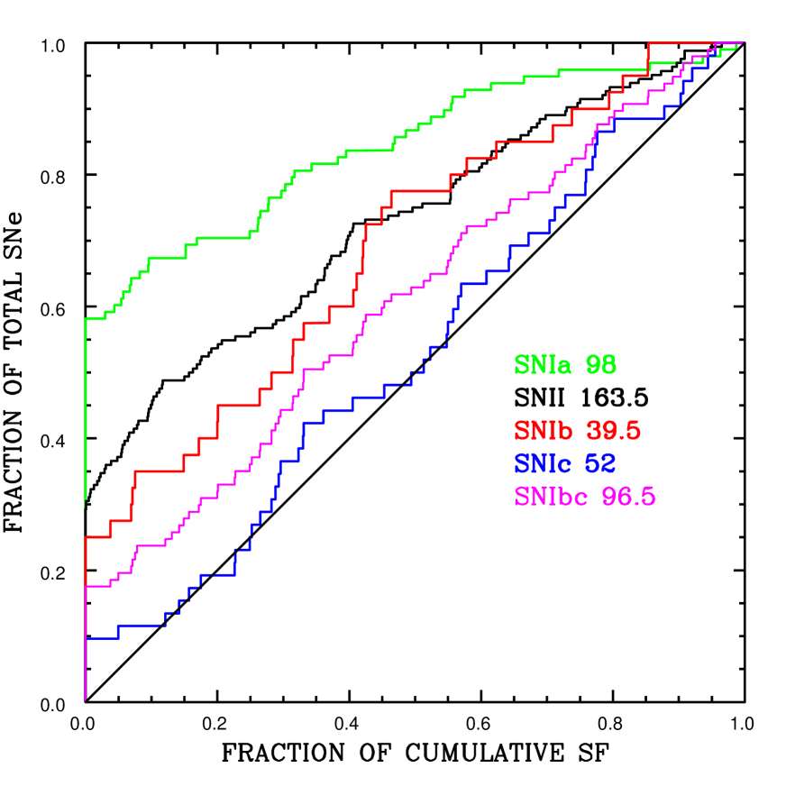
Figure 2: Cumulative pixel statistics plot of all the main SN types. SNIa (98 events) are shown in green, SNII (163.5) in black, SNIb (39.5) in red, the SNIc (52) in blue and the overall SNIbc (96.5) population in magenta. The black diagonal line illustrates a hypothetical, infinite in size distribution that accurately follows the on-going SF. As a distribution moves away to the top left-hand corner from this diagonal it is displaying a lower degree of association to the emission. Hence, a clear sequence is displayed, from the SNIa through the SNII, the SNIb and to the SNIc in terms of increasing association to the H$\alpha$ line emission.

SN type	N	Mean NCR	Std. err.
Ia	98	0.157	0.026
II	163.5	0.254	0.023
Ib	39.5	0.318	0.045
Ic	52	0.469	0.040
Ibc	96.5	0.390	0.031

Table 1: The NCR pixel statistics for each of the ‘main’ SN types. In the first column we list the SN type, followed by the number of events within that distribution in column 2. In column 3 we list the mean NCR value for each SN type, followed finally by the standard error on that mean. Note, there are more SNIbc than the sum of the SNIb and SNIc. This is because there are 5 events in our sample where only a ‘Ib/c’ classification is given in the literature.

The results of the pixel statistics analysis, with respect to host galaxy on-going SF (as traced by H$\alpha$ emission) are presented in table A1, along with SN types, galaxy properties and references.
First, we present results and distributions for the ‘main’ SN types of SNIa, SNII, SNIb and SNIc, while also grouping the SNIbc together (we present the SNIa distribution here for comparison to the CC SNe, however a full analysis and discussion of this distribution, splitting the population by light-curve parameters is being presented elsewhere; Anderson et al., in preparation). The mean NCR values for each distribution are presented in table 1 together with standard errors on the mean and the number of events in each sample. The distributions of each SN type are displayed in Fig. 2 as cumulative distributions.
We use the Kolmogorov-Smirnov (KS) test to probe differences between the distributions, and also between the distributions and a hypothetical, infinite in size flat distribution (i.e. one that accurately traces the SF of its host galaxies). This hypothetical distribution is shown by the diagonal black line in Fig. 2. The results of these tests are now listed, where a percentage is given for the likelihood that two populations are drawn from the same underlying distribution. If this percentage is higher than 10% then we conclude that there is no statistically-significant difference between the distributions.
Ia-II: $\sim$0.1%
II-Ib: $>$10%
Ib-Ic: $\sim$5%
II-Ibc $\sim$0.5%
Probability of being consistent with a flat distribution
II-flat: $<$0.1%
Ib-flat: $<$0.1%
Ic-flat: $>$10%
Ibc-flat: $\sim$0.5%
We find that SNIa show the lowest degree of association to host galaxy SF of all SN types, as expected if these SNe arise from WD progenitor stars, i.e. an evolved stellar population. Following the SNIa we find a sequence of increasing association to the on-going SF, which implies a sequence of decreasing progenitor lifetime and hence an increasing progenitor mass, if we make the simple assumption that a higher degree of association to SF equates to shorter ‘delay-times’ (time between epoch of SF and epoch of SN). This sequence progresses as follows:

SNIa $\Rightarrow$ SNII $\Rightarrow$ SNIb $\Rightarrow$ SNIc

The SNIc appear to arise from the highest mass progenitors of all CC SN types (indeed higher mass also than any of the other sub-types, given the mean values presented below). We note that while the SNIc accurately trace the on-going SF the SNIb do not, while statistically the SNIb show a similar degree of association to the SF as the overall SNII population.
When comparing the overall SNII and SNIbc populations we find that the latter show a significantly higher degree of association to the H$\alpha$ line emission. This implies that overall SNIbc arise from more massive progenitors than the SNII population. We note here that this does not necessarily imply single star progenitors for SNIbc. Our result solely implies that the SNIbc arise from shorter lived, higher mass progenitors, whether single or binary star systems. This issue is discussed in detail below. While all of these results were indicated in our earlier study (AJ08), the current data set is the first to clearly separate out the SN Ib from the SN Ic, with the latter now being seen to be significantly more strongly associated with on-going SF, and hence arising from higher mass progenitors.

4.1 CC SN sub-types

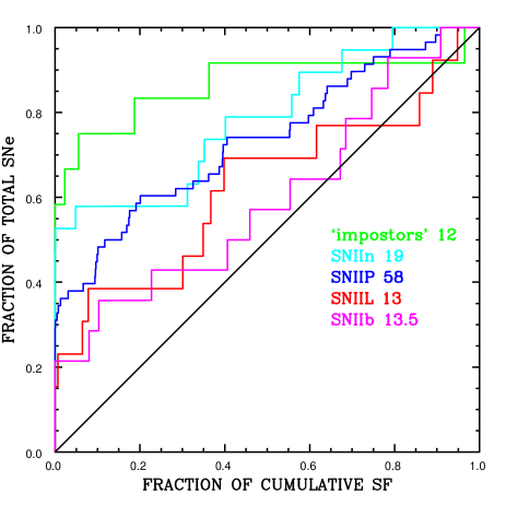
Figure 3: Cumulative pixel statistics plot of the CC SNII sub-types. SN ‘impostors’ (12 events) are shown in green, SNIIn (19) in cyan, SNIIP (58) in blue, SNIIL (13) in red, and SNIIb (13.5) in magenta. As in Fig. 2, lines that are further away from the black diagonal line show a lower degree of association to the on-going SF. Note, the surprising distributions of the SN ‘impostors’ and SNIIn, both of which lie towards the top left hand side of the figure.

SN type	N	Mean NCR	Std. err.
‘impostors’	12	0.133	0.086
IIn	19	0.213	0.065
IIP	58	0.264	0.039
IIL	13	0.375	0.102
IIb	13.5	0.402	0.095

Table 2: The NCR pixel statistics for each of the SNII sub-types. In the first column we list the SN type, followed by the number of events within that distribution in column 2. In column 3 we list the mean NCR value for each SN type, followed finally by the standard error on that mean.

We now further separate the CC SN types into various sub-type classifications that are given in the literature and were discussed earlier in the paper. The mean NCR pixel values together with their standard errors for the CC sub-types are presented in table 2, while we show the cumulative distributions of the different populations in Fig. 3.
We perform KS tests between various distributions together with tests between populations and a hypothetical flat distribution that directly traces the on-going SF. We now list these probabilities:
IIb-IIP: $>$10%
IIn-IIP: $>$10%
Probability of being consistent with a flat distribution
‘impostors’-flat: $<$0.1%
IIn-flat: $<$0.1%
IIP-flat: $<$0.1%
IIL-flat: $\sim$10%
IIb-flat: $>$10%
Again we can list these in terms of increasing association to the H$\alpha$ emission, as is displayed in Fig. 3 (however given the lower number of events within these distributions, the overall order of the sequence may not be intrinsically correct). We find the following sequence of increasing association to the line emission, implying a sequence of increasing progenitor mass:

‘impostors’ $\rightarrow$ IIn $\rightarrow$ IIP $\rightarrow$ IIL $\rightarrow$ IIb

The first observation that becomes apparent looking at this sequence and the distributions displayed in Fig. 3 is the position of the SN ‘impostors’ and the SNIIn. Indeed we find that $>$50% of the SNIIn do not fall on regions of detectable on-going SF (we will soon evaluate the physical meaning of this statement). These observations are perhaps surprising given the substantial literature claims that the progenitors of both of these transient phenomena are Luminous Blue Variable (LBV) stars. LBVs are massive, blue, hot stars that go through some extreme mass-loss events (Humphreys & Davidson, 1994). These pre-SN eruptions may provide the CSM needed to explain the signatures of interaction observed for these transients. However, these claims are inconsistent with their lower association to SF.
Regarding the other sub-types, we find that the SNIIP show a very similar degree of association to the on-going SF as the overall SNII distribution presented above. This is to be expected as a) the overall distribution is dominated by SNIIP and b) it is likely that a large fraction of the SNe simply classified as ‘II’ (48) in the literature are also SNIIP. The fact that a large fraction of the SNIIP population does not fall on regions of on-going SF suggests that large fraction of these SNe arise from progenitors at the lower end to the CC mass range.
The other sub-types included in this study are the SNIIL and SNIIb. Given the low number statistics involved (13 IIL and 12.5 IIb), definitive results and conclusions are perhaps premature. However, it may be interesting to note that both of these types appear to occur within or nearer to bright HII regions than the SNIIP, implying higher mass progenitors.

4.2 SNIIP H$\alpha$ vs near-UV

The mean NCR value for the 58 SNIIP with respect to H$\alpha$ is (as above) 0.264 (standard error on the mean of 0.039). This mean value together with the KS statistic test comparing the population to a flat distribution, shows that the SNIIP do not trace the SF as traced by H$\alpha$ emission. Indeed around 30% of these events fall on pixels containing no H$\alpha$ emission. If we assume that this implies that SNIIP arise from lower mass massive stars then we expect to see a stronger association to the recent SF as traced by near-UV emission. We test this using $GALEX$ near-UV host galaxy imaging and the resulting distribution is shown in Fig. 4 (for the 50 SNIIP from our sample where near-UV images are available). We also list the near-UV NCR values in table 3 together with their H$\alpha$ counterparts and host galaxy information.
We find that the SNIIP accurately trace the near-UV emission (although there are still almost 15% of events that do not fall on regions of SF down to the detection limits of $GALEX$ in the near-UV). The SNIIP near-UV NCR distribution is formally consistent (chance probability $>$10%) with being drawn from a flat distribution (i.e. accurately tracing the recent SF), while the distributions with respect to the on-going and recent SF are statistically not drawn from the same underlying population (KS test probability $<$0.1%). As above, this implies that SNIIP arise from the lower mass end of stars that explode as CC SNe (actual stellar age/mass limits are discussed below).

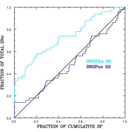
Figure 4: Cumulative plot for the pixel statistics of 50 SNIIP with respect to H$\alpha$ (cyan) and $GALEX$ near-UV emission (blue). While the SNIIP do not accurately trace the youngest SF measured by H$\alpha$ line emission they do follow the near-UV emission which traces SF down to older population ages.

4.3 SNIIn H$\alpha$ vs near-UV

As discussed above the SNIIn show an even lesser degree of association to the H$\alpha$ line emission than the SNIIP, with $>$50% of events having an NCR value of 0. Therefore, as for the SNIIP we re-do the NCR analysis using $GALEX$ near-UV galaxy imaging (using 18 SNIIn with available data). We list the near-UV NCR values in table 4 together with their H$\alpha$ counterparts and host galaxy information. We find a similar trend to that of the SNIIP; the SNIIn are formally consistent ($>$10%) with being randomly drawn from the distribution of recent SF, although we note a larger number of events (than the SNIIP) that fall on regions of zero near-UV emission (22% compared to 14% for the SNIIP). While there appears in Fig. 5 an obvious difference between the SNIIn distributions with respect to the two SF tracers, given the relatively small number of events in each sample a KS test is not conclusive. These results imply that the majority of SNIIn arise from relatively low mass progenitors.

SN	Galaxy	V${}_{\textit{r}}$ (kms-1)	NCRha	NCRuv
SNIIP
1936A	NGC 4273	2378	0.362	0.395
1937F	NGC 3184	592	0.000	0.000
1940B	NGC 4725	1206	0.000	0.000
1948B	NGC 6946	40	0.387	0.934
1965H	NGC 4666	1529	0.597	0.695
1965N	NGC 3074	5144	0.031	0.000
1965L	NGC 3631	1156	0.001	0.551
1969B	NGC 3556	699	0.191	0.219
1969L	NGC 1058	518	0.000	0.562
1971S	NGC 493	2338	0.174	0.617
1972Q	NGC 4254	2407	0.405	0.492
1973R	NGC 3627	727	0.325	0.218
1975T	NGC 3756	1318	0.000	0.102
1982F	NGC 4490	565	0.095	0.549
1985G	NGC 4451	864	0.641	0.933
1985P	NGC 1433	1075	0.000	0.135
1986I	NGC 4254	2407	0.000	0.914
1988H	NGC 5878	1991	0.000	0.000
1989C	UGC 5249	1874	0.689	0.993
1990E	NGC 1035	1241	0.000	0.644
1990H	NGC 3294	1586	0.000	0.270
1991G	NGC 4088	757	0.066	0.231
1997D	NGC 1536	1217	0.000	0.000
1999bg	IC 758	1275	0.632	0.937
1999br	NGC 4900	960	0.099	0.273
1999gi	NGC 3184	592	0.637	0.953
1999gn	NGC 4303	1566	0.897	0.873
2001R	NGC 5172	4030	0.000	0.000
2001X	NGC 5921	1480	0.698	0.543
2001du	NGC 1365	1636	0.101	0.837
2001fv	NGC 3512	1376	0.169	0.282
2002ed	NGC 5468	2842	0.395	0.683
2002hh	NGC 6946	40	0.000	0.653
2003Z	NGC 2742	1289	0.013	0.688
2003ao	NGC 2993	2430	0.157	0.498
2004cm	NGC 5486	1390	0.201	0.638
2004dg	NGC 5806	1359	0.554	0.855
2004ds	NGC 808	4964	0.250	0.678
2004ez	NGC 3430	1586	0.094	0.293
2005ad	NGC 941	1608	0.000	0.261
2005ay	NGC 3938	809	0.873	0.683
2005cs	NGC 5194	463	0.396	0.768
2005dl	NGC 2276	2416	0.730	0.835
2006my	NGC 4651	788	0.553	0.476
2006ov	NGC 4303	1566	0.284	0.885
2007aa	NGC 4030	1465	0.117	0.352
2007od	UGC 12846	1734	0.000	0.000
2008M	ESO 121-g26	2267	0.789	0.925
2008W	MCG -03-22-07	5757	0.005	0.405
2008X	NGC 4141	1897	0.609	0.494

Table 3: List of data for all SNIIP where $GALEX$ near-UV host galaxy images were available in the archive. In column 1 we list the SN name, followed by its host galaxy and recession velocity in columns 2 and 3. We then list the H$\alpha$ NCR values followed by their corresponding near-UV values.

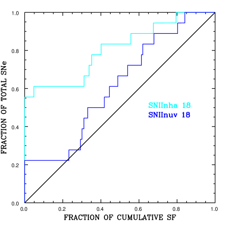
Figure 5: Cumulative plot for the pixel statistics of 18 SNIIn with respect to H$\alpha$ (cyan) and $GALEX$ near-UV emission (blue). While the SNIIn do not accurately trace the youngest SF measured by H$\alpha$ line emission they do follow the near-UV emission which traces rather older populations.

SN	Galaxy	V${}_{\textit{r}}$ (kms-1)	NCRha	NCRuv
SNIIn
1987B	NGC 5850	2556	0.000	0.000
1987F	NGC 4615	4716	0.352	0.541
1993N	UGC 5695	2940	0.000	0.000
1994Y	NGC 5371	2558	0.000	0.331
1994W	NGC 4041	1234	0.795	0.679
1994ak	NGC 2782	2543	0.000	0.311
1995N	MCG -02-38-17	1856	0.001	0.000
1996bu	NGC 3631	1156	0.000	0.000
1997eg	NGC 5012	2619	0.338	0.418
1999el	NGC 6951	1424	0.048	0.232
1999gb	NGC 2532	5260	0.676	0.489
2000P	NGC 4965	2261	0.393	0.620
2000cl	NGC 3318	2775	0.312	0.613
2002A	UGC 3804	2887	0.401	0.803
2002fj	NGC 2642	4345	0.558	0.841
2003dv	UGC 9638	2271	0.000	0.301
2003lo	NGC 1376	4153	0.000	0.293
2006am	NGC 5630	2655	0.000	0.445

Table 4: List of data for all SNIIn where $GALEX$ near-UV host galaxy images were available in the archive. In column 1 we list the SN name, followed by its host galaxy and recession velocity in columns 2 and 3. We then list the H$\alpha$ NCR values followed by their corresponding near-UV values

4.4 SN ‘impostors’ H$\alpha$ vs near-UV

Finally we repeat this analysis of H$\alpha$ against near-UV pixel statistics for the SN ‘impostors’ (11 events). Again we find similar trends that the population shows a higher degree of association to the recent than the on-going SF. We list the near-UV NCR values in table 5 together with their H$\alpha$ counterparts and host galaxy information. Given the low number statistics it is hard to fully trust the results. However, the two distributions as displayed in Fig. 6 suggest that while the ‘impostors’ show a higher degree of association to the near-UV compared to the H$\alpha$ emission, they are not accurately tracing the recent SF. Indeed, using a KS test we find only $\sim$3% chance probability that these events are drawn from the underlying distribution of near-UV emission. This either implies that these events arise from much lower mass progenitors than all other transients studied here, that there is some strong selection effect against finding these events within bright HII regions, or that the stellar birth processes of these objects differ from those which form ‘normal’ massive stars.
We have not chosen to pursue investigations of the correlation of all other types with near-UV emission. We chose the SNIIP, IIn and ‘impostors’ for study because these were the obvious events of interest, given their non-association to the H$\alpha$ emission.

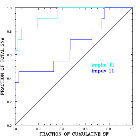
Figure 6: Cumulative plot for the pixel statistics of 11 SN ‘impostors’ with respect to H$\alpha$ (cyan) and $GALEX$ near-UV emission (blue). The ‘impostors’ do not accurately follow the youngest SF measured by H$\alpha$ emission, and while they display a higher association to the near-UV emission they do not appear to accurately trace it.

SN	Galaxy	V${}_{\textit{r}}$ (kms-1)	NCRha	NCRuv
SN ‘impostors’
1954J	NGC 2403	131	0.187	0.738
1961V	NGC 1058	518	0.363	0.000
1997bs	NGC 3627	727	0.023	0.328
1999bw	NGC 3198	663	0.000	0.466
2001ac	NGC 3504	1534	0.000	0.000
2002bu	NGC 4242	506	0.000	0.000
2002kg	NGC 2403	131	0.055	0.654
2003gm	NGC 5334	1386	0.000	0.468
2006fp	UGC 12182	1490	0.000	0.000
2008S	NGC 6946	40	0.031	0.000
2010dn	NGC 3184	463	0.000	0.762

Table 5: List of data for all SN ‘impostors’ where $GALEX$ near-UV host galaxy images were available in the archive. In column 1 we list the SN name, followed by its host galaxy and recession velocity in columns 2 and 3. We then list the H$\alpha$ NCR values followed by their corresponding near-UV values

4.5 Progenitor age and mass constraints

The most robust results presented here are the relative differences between the distributions of the different SN types with respect to host galaxy SF. However, given estimates of the SF ages traced by the two wave-bands used in our analysis, we can go further and make some quantitative constraints.
Earlier, we defined the H$\alpha$ to be tracing the on-going SF, on timescales of less 16 Myr, while defining the near-UV to be tracing recent SF on timescales of 16-100 Myr (both timescales are taken from Gogarten et al. 2009). Hence, we can use these timescales to quantitatively constrain the ages (and hence masses) of different progenitors. We do this by simply asking if a SN distribution accurately traces (i.e. a KS test between a SN population and a ‘flat’ distribution gives a probability of $>$10%) either the on-going or recent SF and then apply the above timescales to the results. We then use table 1 from Gogarten et al. (2009), taken from the models of Marigo et al. (2008) to obtain progenitor mass constraints. As above, the constraints we present below are based on the assumption that a decreasing association to SF equates to longer lived, less massive progenitors.
Before proceeding we need to make an important caveat to the results presented in this subsection. While it is generally accepted that near-UV emission traces SF on timescales longer than that of H$\alpha$, the definitive timescales we present above are less secure. While it may be that stars with ages $\sim$16 Myr produce a small amount of ionizing flux, contributing to that which produce HII regions, the flux will be dominated by the most massive stars. Hence, it has been argued (P. Crowther, private communication 2012) that only the most massive stars will be found to reside within large HII regions. Therefore it could be that only stars with much shorter timescales than 16 Myr accurately trace the spatial distribution of H$\alpha$ emission within galaxies. However, these much higher mass (shorter lifetime) values have not been convincingly shown observationally. Hence, in this section we continue with the age (and therefore mass) ranges that we take from Gogarten et al. (2009) (which were for one environment within one SF galaxy). Finally, we stress that our main results and conclusions are not dependent on the strength of these age limits.
The positions of SNIIP within host galaxies show that they accurately trace the recent and not the on-going SF. Hence we can put an upper limit for the majority of SNIIP to arise from progenitors with ages $>$ 16 Myr and masses $<$ 12${\rm\ M}_{\odot}$ (given the age to mass conversions in table 1 from Gogarten et al. 2009). We note that the upper mass constraint does not exclude progenitor masses above 12${\rm\ M}_{\odot}$, just that the majority will be produced from stars below this mass. Given the shape of the IMF (e.g. Salpeter 1955), even if the possible range of progenitors extends out to above 20${\rm\ M}_{\odot}$ we still expect the majority to be from the low mass end. This is consistent with the direct detections thus far for SNIIP (see Smartt 2009 for a review).
Moving next to the SNIc, these events accurately trace the on-going SF and hence the shortest lived, most massive stars. Using the timescale above we constrain these progenitors to be above 12${\rm\ M}_{\odot}$, hence more massive than the SNIIP. Given that the masses of these SNe if they arise from single stars are probably more than 25${\rm\ M}_{\odot}$ (from observational upper limits of red supergiants; Levesque et al. 2007, and predictions from single star models; e.g. Heger et al. 2003; Eldridge & Tout 2004; Georgy et al. 2009), this constraint does not allow us to differentiate between single and binary star scenarios.
In Fig. 2 we see that the SNIb fall in between the SNIc and SNII in terms of their association to the on-going SF. Indeed they are inconsistent with being drawn from the H$\alpha$ emission distribution. As with the SNIIP, if we take the limits for the production of HII regions detected through H$\alpha$ as 16 Myr then this would constrain the majority of SNIb progenitors to be stars less massive than $\sim$12${\rm\ M}_{\odot}$. Keeping the insecure nature of this mass limit in mind, this would then constrain SNIb to arise from binaries (e.g. Podsiadlowski et al. 1992), as single stars less massive than $\sim$25${\rm\ M}_{\odot}$ are not thought to be able to lose their hydrogen envelopes prior to SN (e.g. Heger et al. 2003; Eldridge & Tout 2004; Georgy et al. 2009).
Given the small statistics for the SNII sub-types, quantitative constraints are more difficult. Therefore we only apply this argument to the SNIIn. The SNIIn do not (KS probability $<$0.1%) trace the on-going SF, and hence as for the SNIIP, this argues that the majority of the events within our sample had progenitor stars with ages of more than 16 Myr and therefore masses of less than 12${\rm\ M}_{\odot}$.

4.6 SNe falling on ‘zero’ star formation

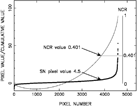
Figure 7: Example of the formation of the NCR pixel statistic (figure reproduced from James & Anderson 2006). The thicker black curve shows the distribution of increasing pixel count, while the thinner curve shows the corresponding cumulative distribution. On the right a scale is shown to represent the NCR values of these distributions. We show this here to draw attention to how this statistic is formed with respect to sky or zero detected emission pixels.

The above analysis has shown that many CC SNe do not fall on regions of on-going and/or recent SF. Here we investigate this further and determine whether this is due to our detection limits or whether there is a significant fraction of events that do indeed explode away from HII regions. This can be achieved by evaluating SN pixel values and determining where these fall in the overall NCR pixel distribution. In Fig. 7 (taken from James & Anderson 2006) we show an example of how the NCR statistic is formed in relation to the rank of the pixels of the host galaxies and their cumulative distributions.
The NCR statistic is formed by ranking all pixels of the host galaxy, including those from the surrounding sky, into a sequence of increasing pixel count. From this count the cumulative distribution is formed. The NCR statistic is considered to have a non-zero value when this distribution becomes positive. In Fig. 7, this occurs where the thin line crosses the cumulative value of zero, where the thick line of individual pixel values has a small but non-zero positive value. Therefore there are many positive pixel counts that have an NCR value of zero. Hence, in forming the NCR statistic we are effectively putting a limit per pixel for detection of emission. This means that there will be pixels which correspond to an NCR value of zero but contain emission, just emission that falls below our detection limit. Now, we can evaluate the cases where a SN has an NCR value of zero and see where this lies within the pixel distribution that is considered as zero. If indeed these SNe are arising from regions consistent with zero intrinsic SF then the distribution of these NCR=0 pixel counts should be evenly distributed either side of zero (the mean sky flux in this statistic).
We do this analysis for the 15 SNIIP that fall on zero H$\alpha$ NCR values. We determine the pixel count on which the SN falls and normalise this so that for each SN we have a value between -1 and 1, where a value of -1 means that the SN falls on the most negative count of the image, and a value of 1 means that the SN falls on the most positive count before the NCR distribution becomes non-zero. We plot the resulting distribution in Fig. 8. We find that the distribution is indeed biased towards positive pixel values. If the SNe were consistent with being drawn from sky or true zero emission pixels we would expect the same number to have negative and positive pixel values within the NCR=0 distribution. Given that there are 3 SNe with negative values and 12 with positive values we find an excess of 9 SNe which fall on zero NCR values but fall on emission which is below our detection limits.
There is no way of knowing which of these 12 positive values are the 9 which fall on intrinsic emission. To estimate the detection limits per pixel of our imaging (and hence our NCR statistic), we estimate SF rates (SFRs) per SN containing pixel. For 5 of the galaxies SFRs have been published in James et al. (2004). For these we take the count for the SN containing pixel and divide this by the overall galaxy H$\alpha$ count. This then gives us a scaling factor to apply to the SFR of the host which we use to calculate a SFR for the SN containing pixel. We use these 5 ‘calibrated’ galaxies as representative of the overall sample of 12 galaxies (this is reasonable given that the SN to total pixel counts ratio is very similar between the ‘calibrated’ and ‘uncalibrated’ samples). The mean SFR in SN containing pixels is 2.1$\times$10^-5 solar masses per year. We assume this to be our NCR median detection limit for our H$\alpha$ imaging. Hence, when we are talking about a certain fraction of a SN population that fall on ‘zero NCR’ values, we are talking about the fraction of events that fall on pixels consistent with (on average) SFRs of around, or below 2.1$\times$10^-5 ${\rm\ M}_{\odot}$ per year. For reference the SFR for the Orion nebula is $\sim$7.9$\times$10^-5 (taking the H$\alpha$ luminosity from Kennicutt 1984, and converting to a SFR using eq. 2 from Kennicutt 1998). Therefore, within the median of our SNIIP host galaxies, we would expect to detect SF regions of the size/luminosity of Orion, but not those with smaller SFRs.

Figure 8: Histogram showing the distribution of the normalised pixel values for the 15 SNIIP which have H$\alpha$ NCR value equal to zero. If these SNe really were falling on regions of zero intrinsic H$\alpha$ emission then we would expect this distribution to be evenly distributed between -1 and 1. As the displayed distribution is clearly biased towards positive pixel values this shows that some of these SNe fall on emission which is not detected in our imaging.

A small number of SNe (IIP, IIn and ‘impostors’) also fall on zero near-UV NCR values. Hence, we ask the same question as above, whether these are really SNe that are falling on zero SF or whether this is simply a detection sensitivity issue.
On inspection of the images used it is clear that we cannot form the same distribution as displayed in Fig. 8. This is because the vast majority of $GALEX$ ‘sky’ pixel counts are simply zero (meaning that when one subtracts the mean sky value an image is left with many negative count pixels of the same value). Duplicated values are unhelpful for proceeding with the analysis presented above for H$\alpha$. Therefore, here we simply calculate whether the pixel where each SN falls is positive or negative.
For the combined sample of SNIIP, IIn and ‘impostors’ there are 16 SNe which fall on zero near-UV NCR pixels. We find that 10 have positive sky values and 6 have negative counts. Taking the number of ‘negative’ SNe as 6 means that there will also be 6 ‘positive’ SNe that are falling on regions consistent with zero emission. Therefore there are only 4 SNe which do fall on regions of emission, but that which is below our detection limits. We conclude that there is a small but not insignificant number of CC SNe which fall on regions of zero intrinsic SF as traced by H$\alpha$ and $GALEX$ near-UV emission.
One may ask the question of whether the differences between the degree of association of the different SN types to host SF are merely due to the overall number of events which fall on NCR=0 pixels. Indeed, when we look at Fig. 2 we see both a sequence of populations moving away from the flat distribution, while also seeing a sequence of NCR=0 fractions when looking only at the y-axis (the position where each distribution starts from the left hand side of this plot gives the fraction of events within the distribution that fall on NCR=0 pixels). To investigate whether additionally there are differences in the shape of each distribution, we re-plot the populations removing these NCR=0 objects. The resulting cumulative distributions are shown in Fig. 9. We see that there still appears to be a sequence of increasing association to the on-going SF within these samples. The KS test of the modified SNII and SNIc distributions indicates that these are still significantly different, at the 2.5% level, while both the SNII and SNIb populations are still not consistent with being drawn from a flat distribution (probabilities of $<$0.1% and $\sim$5% respectively). We therefore observe that SNII and SNIb show both a higher fraction of events falling on zero on-going SF and less frequently explode within bright HII regions than SNIc.

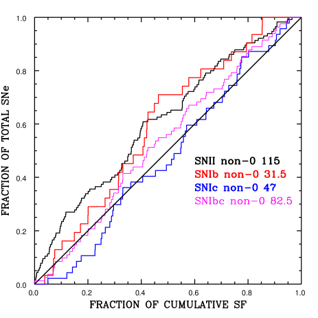
Figure 9: Cumulative pixel statistics with respect to H$\alpha$ host galaxy emission for the main CC SN types, with those NCR values equal to zero removed. SNII (115 events) are shown in black, SNIb (31.5) in red, SNIc (47) in blue, and the overall SNIbc sample (82.5) in magenta. We see that even when these zero values are removed differences remain between the distributions.

4.7 Selection effects and possible sample biases

In this section we test for several possible biases that may be affecting our results. The main result from this paper is, that SNIbc show a higher degree of association to host galaxy on-going SF than SNII. The SNII sample is dominated by SNIIP. One possible source of concern is that the peak brightness luminosity function of SNIIP is seen to extend to lower values than SNIbc. While this difference is observed, the mean luminosities for the IIP and Ibc samples presented by Li et al. (2011) are very similar, and the only differences in the distributions concern a faint tail of $\sim$ 30 per cent of SNII. Nevertheless SNIIP may be harder to detect against bright HII regions, and be affected by a selection effect.
If this is strongly affecting our sample then we would expect to see two trends. Firstly, we would expect the SNII to SNIbc ratio to decrease with increasing distance. This is because as one goes to larger distances it becomes harder to detect objects against the background galaxy emission. Given the (possible) luminosity differences between the two samples we may then expect this effect to be worse for the SNIIP than the SNIbc. Secondly, we would expect that for both SNIIP and SNIbc as one goes to larger distances it would become harder to detect both sets of events against bright HII regions. This would then manifest itself as decreasing NCR pixel values for each sample. In the analysis and discussion below we test these hypotheses.

SN type	N	Mean Vr	Median Vr
II	163.5	2183	1566
Ibc	96.5	2833	2513
IIP	58	1697	1484
IIL	13	1285	1238
IIb	13.5	2526	2426
IIn	19	2779	2619
imp	13	852	628
Ib	39.5	2809	2798
Ic	52	2919	2443
II (no sub-type)	47	3080	2407

Table 6: Mean and median recession velocities for the host galaxies of the different SN types. In the first colum the SN group is listed, followed by the number of events within that group in column 2. In column 3 and 4 we list the mean and median host galaxy recession velocities

In table 6 we list the mean and median recession velocities (which equate to distances) of the host galaxies of each sample and sub-sample of SNe analysed within this work. This initial analysis shows that the SNII sample is nearer in distance than that of the SNIbc. This trend is also shown in Fig. 10. However, there is an obvious target selection bias which is affecting these distributions. Namely, as outlined in section 2, our target SNe host galaxies were chosen to give SNe with sub-type classifications. To classify a SN as a Ibc one needs only a spectrum. However, to classify a SN as a bona-fide IIP or IIL one needs a light-curve of reasonable quality. The community is more likely to take the photometry needed to make this distinction for nearby events. Indeed, apart from the ‘impostors’ the SNIIP and SNIIL have the closest host galaxies, while the events only classified as ‘II’ have considerably larger distances. Adding this to the fact that SNIbc are simply rarer and therefore one has to go to further distances to compile a significant sample and this explains the trend seen in Fig. 10.

Figure 10: The SNII to SNIbc ratio as a function of host galaxy recession velocity. The data is simply split into quartiles of recession velocity and the ratio of events is calculated for each bin. Error bars are calculated using Poisson statistics.

Next we split both the SNIIP and SNIbc samples into 4 equal bins of recession velocity. For each of these bins we calculate the mean NCR value. We then plot these NCR distributions in Fig. 11. While we see the obvious offset in recession velocities of the SNIIP and SNIbc described above, both distributions appear to be very flat with host galaxy velocity. Hence, we conclude that there is no selection effect which preferentially detects SNIbc within bright HII regions with respect to SNII.
Armed with this last conclusion we now discuss all the above results in more detail, confident that we are seeing true intrinsic differences in the association of different SNe with host galaxy SF.

Figure 11: The distribution of mean H$\alpha$ NCR values for the SNIIP and SNIbc samples, split into quartiles of recession velocity. The SNIIP are shown in red triangles while the SNIbc are shown in blue squares. Error bars are the standard error on the mean of each sub-sample.

5 Discussion

The major assumption employed in this work is that an increasing association to SF equates to shorter pre-transient lifetimes. This would appear to be the most logical way to interpret these results. Here we delve deeper into the physical causes of these associations and how one can interpret these in terms of various parameters at play within SN host environments. To motivate this discussion we start by outlining different reasons a SN will occur at different distances from HII regions within hosts.
1) Only very massive stars (i.e. larger than 15-20${\rm\ M}_{\odot}$, Kennicutt 1998; Gogarten et al. 2009) produce sufficient quantities of ionizing flux to produce a bright HII region visible as H$\alpha$ line emission. When these stars explode as SNe the HII region from an episode of SF ceases to exist, and hence when lower mass stars from the same SF episode go SN they will do so in an environment devoid of emission. Therefore, the higher mass progenitors will better trace the on-going SF than their lower mass counterparts.
2) Longer lived, lower mass stars have more time to drift away from their places of birth, i.e. HII regions. Therefore, these lower mass progenitors will explode in regions of lower SF density and overall will trace the SF to a lesser degree. This scenario is also important for continuous SF within the same environment. We can envisage continuous SF where SNe from an initial SF episode trigger further formation events. In this scenario the most massive stars have little time pre-explosion to move away from their host HII regions, while lower mass events have an increasingly long duration of time to drift away.
3) Hydrogen gas which is ionized to produce bright HII regions (through recombination) is blown away by winds from the most massive stars, and their subsequent explosions. Hence, even if lower mass stars still have the necessary ionizing flux to produce HII regions, there is simply not enough gas within the environment. Therefore, while the most massive stars are observed to explode within a dense SF region, the lower mass stars explode into a sparse region devoid of H$\alpha$ emission, again producing differences in the degrees of association of different mass stars with HII regions.
4) Stars that are found away from bright HII regions can be ‘runaway’ events with high velocities, and have as such moved considerable distances between epoch of SF and epoch of SN. Lower mass stars are more likely to be influenced by this effect through both the binary-binary (Poveda et al., 1967) and supernova (Blaauw, 1961) proposed formation mechanisms, due to preferential ejection of the lowest mass star in the former, and the lower mass star being ‘kicked’ by the explosion of the higher mass companion in the latter (indeed this scenario has been addressed in detail for SNe progenitors; Eldridge et al. 2011). Hence, as above, SNe produced by lower mass progenitors would be found to occur further away from SF regions than those of higher mass. This scenario was investigated in James & Anderson (2006) to explain the high fraction of SNII exploding away from the on-going SF of host galaxies.
Using these arguments as a base, we now further discuss the progenitor mass constraints and sequences outlined above.

5.1 Progenitor mass sequences

Fig. 2 shows a striking sequence of increasing progenitor mass. This starts with the SNIa arising from the lowest mass progenitors, through the SNII, the SNIb and finally the SNIc arising from the highest mass stars. With respect to the SNIa this is to be expected as these events are considered to arise from WD systems, i.e. those produced by low mass stars. Indeed this has been observed previously, through the presence of SNIa, and absence of CC SNe within old elliptical galaxies (e.g. van den Bergh et al. 2005). The next group in this sequence are the SNII. (Given the dominance of SNIIP we consider this discussion relevant for the overall SNII population but also of that of the SNIIP.) These SNe, while showing the expected increase of association and hence increase in progenitor mass compared to the SNIa, are not seen to trace bright HII regions within hosts. We explain this result with the conclusion that these events arise from the lower end of the mass range of CC SNe. This is strengthened by the fact that these events accurately trace the recent SF.
Next in the sequence we find the SNIb. These SNe only show a slightly higher correlation than the SNII, but the difference between the SNIb and SNIc is significant. Therefore there is a strong suggestion that SNIb arise from less massive progenitor stars than SNIc. The final transients in this sequence are the SNIc. These events are consistent with being drawn randomly from the spatial distribution of on-going SF, and hence are consistent with being produced by stars at the higher end of the CC mass range.
While we believe that this is the first time observationally these mass differences between ‘normal’ CC SNIIP and other types has been convincingly shown, these differences have been previously predicted. Single star models (Heger et al., 2003; Eldridge & Tout, 2004; Georgy et al., 2009) predict that CC events which have lost part of their outer envelopes arise from more massive progenitors than those of SNIIP. These models also predict the overall progenitor mass sequence we have outlined, with SNIb arising from more massive stars than SNIIP, and SNIc arising from even higher mass progenitors. While these mass differences are likely to be more pronounced in single star scenarios, binary system models (Podsiadlowski et al., 1992; Nomoto et al., 1996) also seem to predict some correlation of SN type with progenitor mass. Observationally there have been suggestions of mass differences through previous work on environments (e.g. Van Dyk et al. 1999; Kelly et al. 2008; AJ08), comparison of these environment studies with galaxy models (Raskin et al., 2008), and also hints from direct detection studies which will be discussed below. However, the study of a large number of SNe and their host environments we present here, together with the use of H$\alpha$ imaging tracing only the sites of the most massive stars, significantly strengthen this progenitor mass sequence picture.

5.2 The SNIIn and ‘impostors’

Probably the most surprising results to emerge from this study (although this was already shown in AJ08) is the low correlation of SN ‘impostors’ and SNIIn with host galaxy SF. This is shown in Fig. 3 and the sub-type progenitor mass sequence outlined in section 4.1. The general consensus is that both of these transients have LBV progenitor stars. This is because of the high mass loss rates needed to provide the CSM required to produce the observed signs of interaction. It has been claimed (see e.g. Smith 2008) that only the most massive stars going through eruptive stages of mass-loss can provide this material. Also, a number of authors have linked LBVs to individual SNIIn and SN ‘impostors’ (e.g. Trundle et al. 2008; Smith et al. 2010; Kiewe et al. 2012), while the one direct detection of a SNIIn that exists points to a very massive star (Gal-Yam et al., 2007). However, the validity of associating the majority of these transients with LBV progenitors has been questioned by Dwarkadas (2011) and Kochanek et al. (2012). Indeed, it appears that the SNIIn and ‘impostor’ family is extremely heterogenous with the possibility of a significant fraction arising from lower mass stars in dusty environments (e.g. Thompson et al. 2009; Kochanek et al. 2012). Unfortunately our sample sizes of these events are too small to further separate them. For both SNIIn and SN ‘impostors’ we find that they do not trace HII regions within their galaxies and this implies that the majority of these events arise from relatively low mass progenitors. This result would seem to be inconsistent with the majority of these transients arising from very high mass stars. We note that this does not exclude a small fraction events such as SN2005gl (Gal-Yam et al., 2007), arising from very massive stars.
While SNIIn are generally considered to be part of the CC SN family, there have been several claims in the literature of SNIa-like events showing strong signs of interaction with a dense CSM. For two SNe; 2002ic (Hamuy et al., 2003) and 2005gl (Aldering et al., 2006) it has been argued that they are part of a hybrid ‘Ia-IIn’ classification. While it seems unlikely that all SNIIn arise from thermonuclear explosions, the possibility remains that there are further cases of SNIa events which are linked to SNIIn, but their spectral features are hidden beneath the continuum dominated spectra observed for interaction driven SNIIn. This discussion is driven by our results that SNIIn show a lesser degree of association to SF than SNIIP, with the distribution lying between those of SNII and SNIa as shown in Fig. 12. This result could be naturally explained if a significant fraction of SNIIn had progenitors consistent with SNIa events; i.e. lower mass than those which explode through CC. While further examples of this hybrid class are needed to strengthen these arguments, we find the distributions as shown in Fig. 12 intriguing; those of SNIIn and SNIa are very similar, and statistically are consistent with being drawn from the same parent population (KS probability $>$10%).

Figure 12: Cumulative pixel statistics with respect to H$\alpha$ host galaxy emission for the SNIa (97 events) shown in green, the SNIIn (19) in cyan, and the SNII (163.5) shown in black. The SNIIn distribution falls almost exactly in the middle of the SNIa and SNII populations.

If one wishes to retain high mass LBV stars as the progenitors of both the ‘impostors’ and SNIIn then one needs to find reasons why some high mass stars explode far from HII regions. Indeed, Smith et al. (2011) specifically predict that SNIIn, given the assumption of LBV progenitors, will be found to occur closer to HII regions than SNIIP. One could hypothesize that we do not observe these transients near to bright HII because the gas geometry is such that the transients are observed but the tracers we use of SF are not. It follows that one would, in addition, observe these events explode outside near-UV traced SF regions. However, earlier we showed that they follow near-UV emission of their host galaxies better than H$\alpha$. If this were an issue of dust extinction we may expect it to be worse at UV wavelengths (than in the optical where we detect H$\alpha$). This closer association to near-UV emission appears to strengthen the conclusion that these events are arising from lower mass progenitors.
For the SN ‘impostors’ there is one strong caveat to these conclusions. Events classified as ‘impostors’ are generally at the low end of the CC luminosity function. Hence, there will be a strong selection effect against finding these transients within bright background regions (this is seen in the median recession velocity of these transients within our sample as listed in table 6). However, we note that if this were the case, and the ‘impostors’ intrinsically followed distributions of high mass stars, this would imply that even in very nearby galaxies we are missing the vast majority of these events, and therefore that the SN ‘impostor’ rate is considerably higher than assumed. For the SNIIn this effect does not appear a viable option as these events are often brighter than ‘normal’ SNII.

5.3 Comparison with Smith et al. (2011)

Smith et al. (2011) recently used local SN rates from the Lick Observatory Supernova Search (Li et al., 2011) to investigate mass ranges for different SN types by comparison to a standard IMF, and attempted to constrain whether single stars, binary systems or a hybrid of both could best explain nearby SN rates. These authors concluded that single stars cannot account for the relative rates of different CC SNe. They tested various scenarios and suggested mass constraints for different SN types. In their favoured scheme (a hybrid of single and binary systems, their Fig. 7) SNIIP, SNIIL and SNIIn are produced by single stars and form a sequence of increasing progenitor mass. SNIIb and SNIb are produced by binaries and form over the entire CC mass range. Finally SNIc are produced by both single and binary systems and have progenitors of high mass. We now discuss each SN type in turn with respect to our results.
SNIIP arise from the lowest mass bin in all scenarios of Smith et al., which is consistent with our results. In their preferred scenario, SNIIL trace slightly higher mass stars than SNIIP, again consistent with our results and the mass sequence presented in section 4.1. In all presented scenarios these authors predict (or assume) that SNIIn arise from higher mass progenitors than SNIIP. We see the opposite trend with the SNIIn showing the lowest degree of association to the on-going SF. Smith et al. constrain SNIIb to arise from binaries from the entire CC mass range. Our results suggest that these SNe arise from higher mass stars than both the SNIIP and SNIIL, but given the low numbers, it is hard to discriminate between different scenarios. SNIb arise from moderately massive stars in both our and their mass sequences, while SNIc arise from the most massive stars. We conclude that overall our results are consistent with those of Smith et al., and their hybrid scenario of single and binary progenitors, with one major exception; the SNIIn.

5.4 Consistency with direct detections and previous results

In the introduction we outline the method of ‘direct detections’ for constraining SN progenitor masses. This technique affords much information on individual events, but is restricted by small number statistics. Here we compare those results with those currently presented. The only type of CC SN to be studied in a statistical sense with relation to direct detections are the SNIIP. Smartt et al. (2009) used the available progenitor mass constraints (plus upper limits) to estimate lower and upper limits for SNIIP progenitors of 8.5 and 16.5 ${\rm\ M}_{\odot}$ respectively. Here we have constrained that the majority of SNIIP arise from the low end of the CC mass range. This is completely consistent with the direct detections to date. We note that our results are completely independent of those from Smartt et al. (2009), and hence strengthen the argument for SNIIP progenitor masses extending down to low values. Recently a number of progenitor identifications have been published for SNIIL (Elias-Rosa et al. 2010, 2011, although the clear identification of one as a definitive IIL has been questioned by Fraser et al. 2010). These detections appear to point towards progenitor stars above 15${\rm\ M}_{\odot}$, and also suggest yellow supergiant progenitors rather than the red supergiant progenitors determined for SNIIP (Smartt et al., 2009). Therefore, we are seeing the same trend; SNIIL have higher mass progenitors than SNIIP. A similar trend has been observed for the SNIIb. Two very close explosions have occurred with IIb spectra; SN1993J and SN2011dh. In both cases, whether one assumes a single or binary scenario, the progenitors appear to be in the 15-20${\rm\ M}_{\odot}$ range (Aldering et al., 1994; Maund et al., 2004; Maund & Smartt, 2009; Maund et al., 2011; Van Dyk et al., 2011). In terms of differences to the SNIIP, this appears consistent with our results; SNIIb arise from more massive stars than SNIIP (whether binary or single systems). There are neither enough direct detections, nor SNe within our samples to evaluate differences between the SNIIL and SNIIb.
There has been one definitive direct detection of a SNIIn; SN2005gl (Gal-Yam et al., 2007). This constrained the progenitor star to be extremely massive; $\sim$50${\rm\ M}_{\odot}$. If we were to generalise to the whole SNIIn population and conclude that all SNIIn have similarly massive progenitors this result would seem very inconsistent with our environment constraints. However, SNIIn are extremely heterogenous and different events may have different origins; the evidence of interaction simply betrays the close (circum-stellar) environment into which an event explodes. Hence, it is probable that there exists multiple channels through which transients display SNIIn-type spectra. We therefore conclude that SN2005gl must be a special case, and that the majority of nearby SNIIn have lower mass progenitors, as suggested by our statistics.
Unfortunately we are still awaiting a direct detection of a SNIbc (Smartt, 2009). This lack of detection (there have been a number of upper limits) has been argued as evidence that SNIbc arise from lower mass binary systems and not single stars. However, the low number statistics, plus the uncertain nature of current modelling of WR stars (the possible progenitors of SNIbc; e.g. Gaskell et al. 1986) means that constraints are less reliable than for SNIIP. With a lack of information from direct detections, our work, together with that presented in Kelly et al. (2008), appears to be the only convincing evidence that SNIbc arise from more massive progenitors than SNII.
Besides our own previous work on environments, there have been a number of investigations on the positions of SNe within their host galaxies. Of particular relevance is the work published by Kelly et al. (2008) and Kelly & Kirshner (2011). The first of these works employed a very similar pixel technique to that used by ourselves but using host galaxy $g^{\prime}$-band light in place of H$\alpha$ emission as a tracer of massive stars. They found similar results; the SNIc much more frequently explode on bright $g^{\prime}$-band regions of their hosts, less so the SNIb and even less so the SNII. The similarity of these results is encouraging. Kelly & Kirshner (2011) also looked at colours of environments, finding that the host environments of SNIb and SNIc are intrinsically bluer than those of SNII and use this to argue further for higher mass progenitors, again consistent with the current and previous work using pixel statistics. Finally, these authors found, as we do, that the environments of SNIIn are similar to those of the overall SNII population.

5.5 Progenitor metallicity

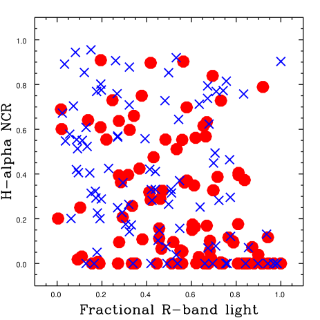
Figure 13: H$\alpha$ NCR pixel values plotted against a normalised parameter tracing the radial location of each SN, with 0 meaning a central location, and 1 meaning an outlying location. The SNIIP plus SNII (all those with no further type classification) are shown as red circles, while the SNIbc are plotted as blue crosses.

Thus far we have not outlined the role of metallicity within our discussion of the implications and conclusions gained from our results. Increased progenitor metallicity is thought to affect the evolution of stars through increasing the metallicity dependent line driven winds and hence increasing the rate of mass loss (e.g. Puls et al. 1996; Kudritzki & Puls 2000; Mokiem et al. 2007). An increase in metallicity could thus increase the ability of a star to lose sufficient amounts of its outer envelope and explode as a SNIbc rather than SNII (see e.g. Heger et al. 2003; Eldridge & Tout 2004; Georgy et al. 2009, for predictions on how the ratio of SN types changes with metallicity). Hence, the effect environment metallicity has on our NCR statistic may need to be taken into account. It has been found by many authors that SNIbc are more centrally concentrated within host galaxies than SNII (e.g. Bartunov et al. 1992; van den Bergh 1997; Tsvetkov et al. 2004; Hakobyan 2008; Boissier & Prantzos 2009; Anderson & James 2009). Until recently these radial differences have been almost exclusively ascribed to metallicity effects, with the central parts of galaxies being more metal rich than the outer environments (see e.g. Henry & Worthey 1999). Therefore one may speculate that higher NCR values for SNIbc (with respect to SNII) are due to the centralisation of these events where more central SNe fall on brighter HII regions. Hence, the hypothesis would be that the relatively higher pixel values for SNIbc is actually a metallicity and not a mass effect. We rule this out on the basis of the following arguments:
a) The validity of the assumption that the brightest regions of SF within galaxies are centralised is unclear. We see within our sample a huge variety of distributions of SF and this is also shown in the 3 example images displayed in Fig. 1. We can see a clear case (that on the right) of a galaxy where the dominant H$\alpha$ regions are in the spiral arms and not the central parts of the galaxy.
b) Habergham et al. (2010) (also see Habergham et al. in preparation; these studies used the same sample we present here) showed that the centralisation of SNIbc is dominated by those SNe occurring within disturbed galaxies, where one observes shallower if any metallicity gradients (Kewley et al., 2010). Therefore, even if there were some correlation between radial position and NCR value, this could not be explained by metallicity.
c) In Anderson et al. (2010), using host HII region spectroscopy of a random subset of the SNe we use for the current sample, we showed that there is no significant metallicity difference between the environments (and hence progenitors) between SNIbc and SNII.
To test this hypothesis further we show in Fig. 13 a scatter plot of the H$\alpha$ NCR values for SNII and SNIbc against the radial positions of each SN with respect to host galaxy $R$-band light (a full analysis of these radial distributions will be presented in Habergham et al. in preparation). If this hypothesis of higher NCR values being centralised were correct, for both samples we would expect to see a clear trend of more events in both the top left and bottom right corners of the plot. While there appears to be some evidence that those SNe having NCR values of 0 are more often found in the outer regions of their hosts (the bottom right part of Fig. 13) this does not seem to be strong, and we see no evidence for the highest pixel counts arising from the most central regions.
We conclude, through the arguments outlined above plus the distributions shown in Fig. 13, that metallicity cannot explain our results of an increased association of SNIbc to SF with respect to SNII.

5.6 Progenitor binarity

A major debate within the SN community currently hinges on whether SNe arising from progenitor stars that have had their envelopes stripped before explosion arise from single or binary star systems. In the single star scenario (see Heger et al. 2003; Eldridge & Tout 2004; Georgy et al. 2009 for such models), stars more massive than 25-30${\rm\ M}_{\odot}$ lose their envelopes through strong stellar winds, the strengths of which are dependent on metallicity. In the binary scenario (see e.g. Podsiadlowski et al. 1992; Nomoto et al. 1996) progenitor masses for the SNIbc (plus SNIIb and possibly SNIIL) extend down further in mass as envelope removal is aided by binary companions. The lack of direct detections of SNIbc would seem to favour binary progenitors, but as we discuss above, thus far this is inconclusive. For at least one CC SN; 1993J, convincing evidence for a binary progenitor system has been observed (Maund & Smartt, 2009).
We conclude that overall the SNIbc population has higher mass progenitor stars than SNII. However, as noted, this does not differentiate between binary or single scenarios. If one envisages an IMF from 8 to 100${\rm\ M}_{\odot}$ with single stars up to e.g. 25${\rm\ M}_{\odot}$ (generally the highest mass red giant stars; Levesque et al. 2007) producing SNIIP (and possibly other SNII), while stars in the full mass range that are binaries explode as SNIbc, then on average progenitors of SNIbc would still be more massive than their SNII counterparts. We speculate here that our results are consistent with SNIb arising from binaries or single stars in an intermediate mass range (above the SNIIP but below the SNIc), with the possibility that SNIc could arise from more massive binaries, very massive single stars, or a combination of both.
A recent study by Eldridge et al. (2011) specifically looked at the production of CC SNe through binaries and how the initially most massive stars explode and ‘kick’ their lower mass companions with velocities meaning that the lower mass stars explode further away from their places of birth than their high mass companions. This is then broadly consistent with the results we find in terms of the increasing association to SF of II to Ib and finally Ic. However, we note that these models only predicted offsets of at most 100 pc from their birth place, distances that are generally not probed by the present study.
A final question that can be asked in this section is whether a change in the percentage of close binaries with environment could explain our results without any need for progenitor mass differences. One may imagine that in denser environments; e.g. bright HII regions, the fraction of close binaries may differ from that in the field. However, we know of no theoretical models or observational constraints which shed light on whether this explanation is feasible, or even on the sense of any such effects. It is possible that the close binary fraction would be higher in denser regions solely because of the higher number of stars in close proximity during SF, but equally, a dense environment may prevent the formation of close binaries. If the fraction of close binaries were higher within HII regions then this could explain our result without resorting to progenitor mass differences. However, we currently see no reason to favour this interpretation over the most logical assumption that an increasing association to HII regions means higher mass progenitor stars.

6 Conclusions

We have presented constraints on the relative progenitor ages, and therefore implied masses of the different CC SN types, using a pixel statistics method applied to H$\alpha$ and near-UV imaging of their host galaxies. Using the assumption that a higher degree of association of a population to host on-going SF means shorter lifetimes we constrained differences in the progenitor masses of CC SNe. Where distributions show a low degree of association to the line emission, we also investigated the association to a longer lived SF component; the recent SF, as traced by near-UV emission. We now list our main results and conclusions achieved with this study.

• SNIbc show a much higher degree of association to the on-going SF of their host galaxies than the SNII. Whether the main progenitor channel for the former is a single or binary scenario, this implies for both channels that SNIbc arise from shorter lived and therefore more massive progenitor stars than SNII.

• Including the SNIa for comparison, we find a strong trend of increasing progenitor mass, starting with the SNIa from the lowest, through the SNII, then the SNIb, with the SNIc arising from the highest mass progenitor stars.

• The SNIc show the highest degree of association of all SNe types, arguing that these SNe arise from the most massive stars that explode as visible transients. Indeed, they are seen to correlate with SF on the shortest timescales much more than the SNIb. This argues that SNIc arise from more massive stars than SNIb.

• While the SNIIP do not follow the underlying distribution of the on-going host galaxy SF, these SNe do follow the distribution of recent SF as traced by near-UV emission. This result suggests that the majority of the progenitors of these SNe populate the lower mass range of massive stars that explode as CC SNe.

• We find that the SNIIn show an even lesser degree of association with the on-going SF than the SNIIP. The most logical explanation for this result is that the majority of these SNe do not arise from the deaths of the most massive stars, in contradiction to several previous studies of these SNe.

Appendix A SN and host galaxy data

SN	Host galaxy	Galaxy type	V${}_{\textit{r}}$ (kms-1)	SN type	NCR value	Telescope	Reference
1936A	NGC 4273	SBc	2378	IIP	0.362	LT
1982R	NGC 1187	SBc	1390	Ib	0.000	LT
1983V	NGC 1365	SBb	1636	Ic	0.330	ESO
1984L	NGC 991	SABc	1532	Ib	0.853	LT
1984F	MCG +08-15-47	Im	2254	II	0.112	JKT	SAI SN catalogue
1984I	ESO 323-G99	SABc	3219	Ib	0.000	ESO
1985P	NGC 1433	SBab	1075	IIP	0.000	ESO
1987B	NGC 5850	SBb	2556	IIn	0.000	ESO
1988H	NGC 5878	SAb	1991	IIP	0.000	LT
1990B	NGC 4568	SAbc	2255	Ic	0.776	JKT
1990I	NGC 4650A		2880	Ib	0.000	ESO
1990W	NGC 6221	SBbc	1499	Ic	0.642	ESO	Van Dyk et al. (1999)
1993N	UGC 5695	S	2940	IIn	0.000	ESO
1994N	UGC 5695	S	2940	II	0.000	ESO
1994W	NGC 4041	SAbc	1234	IIn	0.795	LT	Filippenko & Barth (1994)
1994ai	NGC 908	SAc	1509	Ic	0.523	ESO
1995X	UGC 12160	Scd	1555	II	0.903	LT
1996D	NGC 1614	SBc	4778	Ic	0.361	JKT
1996N	NGC 1398	SBab	1396	Ib	0.315	ESO
1996cr	ESO 97-G13	SAb	434	IIn	0.575	ESO
1997B	IC 438	SAc	3124	Ic	0.644	ESO
1997D	NGC 1536	SBc	1217	IIP	0.000	ESO	Elmhamdi et al. (2003)
1999bg	IC 758	SBcd	1275	IIP	0.632	LT
1999el	NGC 6951	SABbc	1424	IIn	0.048	LT
1999ga	NGC 2442	SABbc	1466	IIL	0.349	ESO
1999go	NGC 1376	SAcd	4153	II	0.363	ESO
2000H	IC 454	SBab	3945	Ib	0.623	ESO	Branch et al. (2002)
2000P	NGC 4965	SABd	2261	IIn	0.000	ESO
2000cl	NGC 3318	SABb	2775	IIn	0.312	ESO
2000fn	NGC 2526	S	4603	Ib	0.282	ESO
2001X	NGC 5921	SBbc	1480	IIP	0.698	LT
2001bb	IC 4319	SAbc	4653	Ic	0.282	ESO
2001db	NGC 3256	Pec	2804	II	0.319	ESO
2001du	NGC 1365	SBb	1636	IIP	0.101	ESO
2002J	NGC 3464	SABc	3736	Ic	0.331	ESO
2002ao	UGC 9299	SABd	1539	Ib	0.000	LT	Pastorello et al. (2008)
2002hc	NGC 2559	SBbc	1559	IIL	0.948	ESO
2002hy	NGC 3464	SABc	3736	Ib	0.411	ESO
2002jp	NGC 3313	SBb	3706	Ic	0.903	ESO
2003I	IC 2481	S	5322	Ib	0.000	ESO
2003dv	UGC 9638	Im	2271	IIn	0.000	LT
2003gm	NGC 5334	SBc	1386	impostor	0.000	LT	Patat et al. (2003)
2003id	NGC 895	SAcd	2288	Ic	0.252	LT
2003lo	NGC 1376	SAcd	4153	IIn	0.000	ESO
2005bf	MCG +00-27-05	SBb	5670	Ib	0.069	ESO
2004cc	NGC 4568	SAbc	2255	Ic	0.608	JKT
2004ch	NGC 5612	SABb	2699	II	0.371	ESO
2004cm	NGC 5486	SAm	1390	IIP	0.201	JKT
2004ds	NGC 808	SABbc	4964	IIP	0.250	ESO
2004ez	NGC 3430	SABc	1586	IIP	0.094	LT
2004gn	NGC 4527	SABbc	1736	Ic	0.558	INT
2005U	ARP 299	IBm/SBm	3088	IIb	0.672	INT
2005bq	IC 4367	SBbc	4090	Ic	0.227	ESO
2005dg	ESO 420-G03	SAbc	4131	Ic	0.249	ESO
2005my	ESO 302-G57	SABc	4441	II	0.839	ESO
2006T	NGC 3054	SABbc	2426	IIb	0.000	LT
2006ba	NGC 2980	SABc	5720	IIb	0.227	ESO
2006bc	NGC 2397	SABb	1363	IIP	0.750	ESO
2006bv	UGC 7848	SABcd	2513	impostor	0.000	LT	Smith et al. (2011)
2006fp	UGC 12182	S	1490	impostor	0.965	LT	Blondin et al. (2006)
2006my	NGC 4651	SAc	788	IIP	0.553	LT
2006lv	UGC 6517	Sbc	2491	Ib/c	0.000	JKT
2007C	NGC 4981	SABbc	1680	Ib	0.264	LT
2007Y	NGC 1187	SBc	1390	Ib	0.000	LT

SN	Host galaxy	Galaxy type	V${}_{\textit{r}}$ (kms-1)	SN type	NCR value	Telescope	Reference
2007aa	NGC 4030	SAbc	1465	IIP	0.117	LT
2007ay	UGC 4310	SAm	4355	IIb	0.000	ESO
2007fo	NGC 7714	SBb	2798	Ib	0.149	LT
2007gr	NGC 1058	SAc	518	Ic	0.157	JKT
2007od	UGC 12846	Sm	1734	IIP	0.000	LT
2007rw	UGC 7798	IBm	2568	IIb	0.784	ESO
2008M	ESO 121-G26	SBc	2267	IIP	0.789	ESO
2008S	NGC 6946	SABcd	40	IIn	0.000	LT	Smith et al. (2011)
2008V	NGC 1591	SBab	4113	IIb	0.685	ESO
2008W	MCG -03-22-07	Sc	5757	IIP	0.005	ESO
2008X	NGC 4141	SBcd	1897	IIP	0.609	LT
2008aq	MCG -02-33-20	SBm	2390	IIb	0.909	ESO
2008bo	NGC 6643	SAc	1484	IIb	0.103	LT	Navasardyan et al. (2008)
2008cn	NGC 4603	SAbc	2592	IIP	0.008	ESO	Elias-Rosa et al. (2009)
2008dv	NGC 1343	SABb	2215	Ic	0.802	LT
2008dw	UGC 8932	Im	3728	II	0.826	JKT
2008ij	NGC 6643	SAc	1484	IIP	0.096	JKT	Challis (2008)
2008im	UGC 2906	Sb	2494	Ib	0.000	LT
2008iz	NGC 3034	I0	203	II	0.496	INT
2009dd	NGC 4088	SABbc	757	II	0.601	JKT
2009kr	NGC 1832	SBbc	1939	IIL	0.890	INT
2009hd	NGC 3627	SABb	727	IIL	0.398	INT	Elias-Rosa et al. (2011)
2009jf	NGC 7479	SBc	2381	Ib	0.464	JKT
2009js	NGC 918	SABc	1507	IIP	0.000	JKT
2010O	ARP 299	IBm/SBm	3088	Ib	0.421	INT
2010P	ARP 299	IBm/SBm	3088	Ib/IIb*	0.406	INT
2010br	NGC 4051	SABbc	700	Ib/c	0.000	INT
2010dn	NGC 3184	SABcd	592	impostor	0.000	INT	Smith et al. (2011)
2011aq	NGC 1056	Sa	1545	II	0.554	JKT
2011ca	NGC 4495	Sab	4550	Ic	0.121	INT
2011dh	NGC 5194	SAbc	463	IIb	0.000	INT
2011fd	NGC 2273B	SBcd	2101	IIP	0.000	JKT

Table 1: SN and host galaxy information for all those ‘new’ SNe analysed in this work (the ‘old’ events being those presented in AJ08). In column 1 we list the SN name followed by its host galaxy in column 2. Then the host Hubble type is given in column 3 and its recession velocity in column 4. The SN type is then listed followed by the H$\alpha$ NCR value. In column 7 we show the telescope used to obtain the observations for that particular host galaxy. Cases where a different SN type was used from that documented on the Asiago catalogue are listed together with a reference in column 8. Note, SN1987B is listed as ‘IInL’ in the Asiago catalogue. Here we put this in the ‘IIn’ class for our investigation. Finally, we note that in AJ08 the NCR values were wrongly listed as 0.000 for SN1964L, SN1986I and SN1999bu. The true values are 0.453, 0.005 and 0.226 respectively.

References

- Aazami & Li (2001) Aazami A. B., Li W. D., 2001, IAUC CBET, 7643, 2
- Aldering et al. (2006) Aldering G., et al., 2006, ApJ, 650, 510
- Aldering et al. (1994) Aldering G., Humphreys R. M., Richmond M., 1994, AJ, 107, 662
- Anderson et al. (2010) Anderson J. P., Covarrubias R. A., James P. A., Hamuy M., Habergham S. M., 2010, MNRAS, 407, 2660
- Anderson & James (2008) Anderson J. P., James P. A., 2008, MNRAS, 390, 1527
- Anderson & James (2009) Anderson J. P., James P. A., 2009, MNRAS, 399, 559
- Arcavi et al. (2010) Arcavi I., et al., 2010, ApJ, 721, 777
- Barbon et al. (1979) Barbon R., Ciatti F., Rosino L., 1979, A&A, 72, 287
- Bartunov et al. (1992) Bartunov O. S., Makarova I. N., Tsvetkov D. I., 1992, A&A, 264, 428
- Bartunov et al. (1994) Bartunov O. S., Tsvetkov D. Y., Filimonova I. V., 1994, PASP, 106, 1276
- Bauer et al. (2008) Bauer F. E., Dwarkadas V. V., Brandt W. N., Immler S., Smartt S., Bartel N., Bietenholz M. F., 2008, ApJ, 688, 1210
- Blaauw (1961) Blaauw A., 1961, BAIN, 15, 265
- Blondin et al. (2006) Blondin S., Masters K., Modjaz M., Kirshner R., Challis P., Matheson T., Berlind P., 2006, Central Bureau Electronic Telegrams, 636, 1
- Boissier & Prantzos (2009) Boissier S., Prantzos N., 2009, A&A, 503, 137
- Branch et al. (2002) Branch D., et al., 2002, ApJ, 566, 1005
- Bruenn et al. (2009) Bruenn S. W., Mezzacappa A., Hix W. R., Blondin J. M., Marronetti P., Messer O. E. B., Dirk C. J., Yoshida S., 2009, Journal of Physics Conference Series, 180, 012018
- Challis (2008) Challis P., 2008, Central Bureau Electronic Telegrams, 1627, 1
- Chevalier (2006) Chevalier R. A., 2006, ArXiv Astrophysics e-prints
- Chugai & Danziger (1994) Chugai N. N., Danziger I. J., 1994, MNRAS, 268, 173
- Dwarkadas (2011) Dwarkadas V. V., 2011, MNRAS, 412, 1639
- Eldridge et al. (2011) Eldridge J. J., Langer N., Tout C. A., 2011, MNRAS, 414, 3501
- Eldridge & Tout (2004) Eldridge J. J., Tout C. A., 2004, MNRAS, 353, 87
- Elias-Rosa et al. (2009) Elias-Rosa N., et al., 2009, ApJ, 706, 1174
- Elias-Rosa et al. (2010) Elias-Rosa N., et al., 2010, ApJ Let., 714, L254
- Elias-Rosa et al. (2011) Elias-Rosa N., et al., 2011, ApJ, 742, 6
- Elmhamdi et al. (2003) Elmhamdi A., Chugai N. N., Danziger I. J., 2003, A&A, 404, 1077
- Filippenko (1997) Filippenko A. V., 1997, ARA&A, 35, 309
- Filippenko & Barth (1994) Filippenko A. V., Barth A. J., 1994, IAUC CBET, 6046, 2
- Filippenko et al. (2003) Filippenko A. V., Chornock R., Swift B., Modjaz M., Simcoe R., Rauch M., 2003, IAUC CBET, 8159, 2
- Filippenko et al. (1993) Filippenko A. V., Matheson T., Ho L. C., 1993, ApJ Let., 415, L103+
- Foley et al. (2009) Foley R. J., et al., 2009, AJ, 138, 376
- Foley et al. (2007) Foley R. J., Smith N., Ganeshalingam M., Li W., Chornock R., Filippenko A. V., 2007, ApJ Let., 657, L105
- Fraser et al. (2010) Fraser M., et al., 2010, ApJ Let., 714, L280
- Fruchter et al. (2006) Fruchter A. S., et al., 2006, Nature, 441, 463
- Gal-Yam et al. (2007) Gal-Yam A., et al., 2007, ApJ, 656, 372
- Gaskell et al. (1986) Gaskell C. M., Cappellaro E., Dinerstein H. L., Garnett D. R., Harkness R. P., Wheeler J. C., 1986, ApJ Let., 306, L77
- Georgy et al. (2009) Georgy C., Meynet G., Walder R., Folini D., Maeder A., 2009, A&A, 502, 611
- Gogarten et al. (2009) Gogarten S. M., et al., 2009, ApJ, 691, 115
- Graham et al. (2003) Graham J., Li W., Puckett T., Toth D., Qiu Y. L., 2003, IAUC CBET, 8045, 1
- Habergham et al. (2010) Habergham S. M., Anderson J. P., James P. A., 2010, ApJ, 717, 342
- Hakobyan (2008) Hakobyan A. A., 2008, Astrophysics, 51, 69
- Hamuy et al. (2003) Hamuy M., et al., 2003, Nature, 424, 651
- Hanke et al. (2011) Hanke F., Marek A., Mueller B., Janka H.-T., 2011, ArXiv e-prints
- Heger et al. (2003) Heger A., Fryer C. L., Woosley S. E., Langer N., Hartmann D. H., 2003, ApJ, 591, 288
- Henry & Worthey (1999) Henry R. B. C., Worthey G., 1999, PASP, 111, 919
- Huang (1987) Huang Y.-L., 1987, PASP, 99, 461
- Humphreys & Davidson (1994) Humphreys R. M., Davidson K., 1994, PASP, 106, 1025
- James & Anderson (2006) James P. A., Anderson J. P., 2006, A&A, 453, 57
- James et al. (2004) James P. A., et al., 2004, A&A, 414, 23
- Jha et al. (2006) Jha S., Branch D., Chornock R., Foley R. J., Li W., Swift B. J., Casebeer D., Filippenko A. V., 2006, AJ, 132, 189
- Kelly & Kirshner (2011) Kelly P. L., Kirshner R. P., 2011, ArXiv e-prints
- Kelly et al. (2008) Kelly P. L., Kirshner R. P., Pahre M., 2008, ApJ, 687, 1201
- Kennicutt (1984) Kennicutt Jr. R. C., 1984, ApJ, 287, 116
- Kennicutt (1998) Kennicutt Jr. R. C., 1998, ARA&A, 36, 189
- Kewley et al. (2010) Kewley L. J., Rupke D., Jabran Zahid H., Geller M. J., Barton E. J., 2010, ApJ Let., 721, L48
- Kiewe et al. (2012) Kiewe M., et al., 2012, ApJ, 744, 10
- Kochanek et al. (2011) Kochanek C. S., Szczygiel D. M., Stanek K. Z., 2011, ApJ, 737, 76
- Kochanek et al. (2012) Kochanek C. S., Szczygiel D. M., Stanek K. Z., 2012, ArXiv e-prints
- Kudritzki & Puls (2000) Kudritzki R.-P., Puls J., 2000, ARA&A, 38, 613
- Leloudas et al. (2011) Leloudas G., et al., 2011, A&A, 530, A95
- Leloudas et al. (2010) Leloudas G., Sollerman J., Levan A. J., Fynbo J. P. U., Malesani D., Maund J. R., 2010, A&A, 518, A29
- Levesque et al. (2007) Levesque E. M., Massey P., Olsen K. A. G., Plez B., 2007, ApJ, 667, 202
- Li et al. (2011) Li W., et al., 2011, MNRAS, 412, 1441
- Marigo et al. (2008) Marigo P., Girardi L., Bressan A., Groenewegen M. A. T., Silva L., Granato G. L., 2008, A&A, 482, 883
- Maund et al. (2006) Maund J. R., et al., 2006, MNRAS, 369, 390
- Maund et al. (2011) Maund J. R., et al., 2011, ApJ Let., 739, L37
- Maund & Smartt (2009) Maund J. R., Smartt S. J., 2009, Science, 324, 486
- Maund et al. (2004) Maund J. R., Smartt S. J., Kudritzki R. P., Podsiadlowski P., Gilmore G. F., 2004, Nature, 427, 129
- Mezzacappa (2005) Mezzacappa A., 2005, Annual Review of Nuclear and Particle Science, 55, 467
- Minkowski (1941) Minkowski R., 1941, PASP, 53, 224
- Modjaz (2011) Modjaz M., 2011, Astronomische Nachrichten, 332, 434
- Modjaz (2012) Modjaz M., 2012, ArXiv e-prints
- Modjaz et al. (2008) Modjaz M., Kewley L., Kirshner R. P., Stanek K. Z., Challis P., Garnavich P. M., Greene J. E., Kelly P. L., Prieto J. L., 2008, AJ, 135, 1136
- Mokiem et al. (2007) Mokiem M. R., et al., 2007, A&A, 473, 603
- Morrissey et al. (2007) Morrissey P., et al., 2007, ApJS, 173, 682
- Navasardyan et al. (2008) Navasardyan H., Benetti S., Harutyunyan A., Agnoletto I., Bufano F., Cappellaro E., Turatto M., 2008, Central Bureau Electronic Telegrams, 1325, 1
- Nomoto et al. (1996) Nomoto K., et al., 1996, in van Paradijs J., van den Heuvel E. P. J., Kuulkers E., eds, Compact Stars in Binaries Vol. 165 of IAU Symposium, The Origin of Type Ib-Ic-IIb-IIL Supernovae and Binary Star Evolution. p. 119
- Nordhaus et al. (2010) Nordhaus J., Burrows A., Almgren A., Bell J., 2010, ApJ, 720, 694
- Pastorello et al. (2008) Pastorello A., et al., 2008, MNRAS, 389, 113
- Patat et al. (2003) Patat F., Pastorello A., Aceituno J., 2003, IAUC CBET, 8167, 3
- Perets et al. (2010) Perets H. B., et al., 2010, Nature, 465, 322
- Perets et al. (2011) Perets H. B., et al., 2011, ApJ Let., 728, L36
- Podsiadlowski et al. (1992) Podsiadlowski P., Joss P. C., Hsu J. J. L., 1992, ApJ, 391, 246
- Poveda et al. (1967) Poveda A., Ruiz J., Allen C., 1967, Boletin de los Observatorios Tonantzintla y Tacubaya, 4, 86
- Prantzos & Boissier (2003) Prantzos N., Boissier S., 2003, A&A, 406, 259
- Prieto et al. (2008) Prieto J. L., Stanek K. Z., Beacom J. F., 2008, ApJ, 673, 999
- Puls et al. (1996) Puls J., et al., 1996, A&A, 305, 171
- Raskin et al. (2008) Raskin C., Scannapieco E., Rhoads J., Della Valle M., 2008, ApJ, 689, 358
- Richter & Rosa (1984) Richter O.-G., Rosa M., 1984, A&A, 140, L1
- Salpeter (1955) Salpeter E. E., 1955, ApJ, 121, 161
- Schlegel (1990) Schlegel E. M., 1990, MNRAS, 244, 269
- Smartt (2009) Smartt S. J., 2009, ARA&A, 47, 63
- Smartt et al. (2009) Smartt S. J., Eldridge J. J., Crockett R. M., Maund J. R., 2009, MNRAS, 395, 1409
- Smith (2008) Smith N., 2008, in IAU Symposium Vol. 250 of IAU Symposium, Episodic Mass Loss and Pre-SN Circumstellar Envelopes. pp 193–200
- Smith et al. (2010) Smith N., et al., 2010, AJ, 139, 1451
- Smith et al. (2011) Smith N., Li W., Filippenko A. V., Chornock R., 2011, MNRAS, 412, 1522
- Smith et al. (2011) Smith N., Li W., Silverman J. M., Ganeshalingam M., Filippenko A. V., 2011, MNRAS, 415, 773
- Thompson et al. (2009) Thompson T. A., Prieto J. L., Stanek K. Z., Kistler M. D., Beacom J. F., Kochanek C. S., 2009, ApJ, 705, 1364
- Trundle et al. (2008) Trundle C., Kotak R., Vink J. S., Meikle W. P. S., 2008, A&A, 483, L47
- Tsvetkov et al. (2004) Tsvetkov D. Y., Pavlyuk N. N., Bartunov O. S., 2004, Astronomy Letters, 30, 729
- van den Bergh (1997) van den Bergh S., 1997, AJ, 113, 197
- van den Bergh et al. (2005) van den Bergh S., Li W., Filippenko A. V., 2005, PASP, 117, 773
- van Dyk (1992) van Dyk S. D., 1992, AJ, 103, 1788
- Van Dyk et al. (2011) Van Dyk S. D., et al., 2011, ApJ Let., 741, L28
- van Dyk et al. (1996) van Dyk S. D., Hamuy M., Filippenko A. V., 1996, AJ, 111, 2017
- Van Dyk & Matheson (2012) Van Dyk S. D., Matheson T., 2012, ApJ, 746, 179
- Van Dyk et al. (1999) Van Dyk S. D., Peng C. Y., Barth A. J., Filippenko A. V., 1999, AJ, 118, 2331
- van Dyk et al. (2000) van Dyk S. D., Peng C. Y., King J. Y., Filippenko A. V., Treffers R. R., Li W., Richmond M. W., 2000, PASP, 112, 1532