H i Power Spectra and the Turbulent ISM of Dwarf Irregular Galaxies

Abstract

H i spatial power spectra (PS) were determined for a sample of 24 nearby dwarf irregular galaxies selected from the LITTLE THINGS (Local Irregulars That Trace Luminosity Extremes – The H i Nearby Galaxy Survey) sample. The two-dimensional (2D) power spectral indices asymptotically become a constant for each galaxy when a significant part of the line profile is integrated. For narrow channel maps, the PS become shallower as the channel width decreases, and this shallowing trend continues to our single channel maps. This implies that even the highest velocity resolution of 1.8 km s^-1 is not smaller than the thermal dispersion of the coolest, widespread H i component. The one-dimensional PS of azimuthal profiles at different radii suggest that the shallower PS for narrower channel width is mainly contributed by the inner disks, which indicates that the inner disks have proportionally more cooler H i than the outer disks. Galaxies with lower luminosity ($M_{B}$ $>$ $-$14.5 mag) and star formation rate (SFR, log(SFR ($M_{\odot}\;{\rm yr}^{-1}$)) $<$ $-$2.1) tend to have steeper PS, which implies that the H i line-of-sight depths can be comparable with the radial length scales in low mass galaxies. A lack of a correlation between the inertial-range spectral indices and SFR surface density implies that either non-stellar power sources are playing a fundamental role in driving the interstellar medium (ISM) turbulent structure, or the nonlinear development of turbulent structures has little to do with the driving sources.

1. Introduction

Pervasive interstellar medium (ISM) turbulence regulates star formation (SF) by creating local density enhancements and countering gravitational collapse. Hierarchical SF (e.g. Efremov & Elmegreen 1998a; Gladwin et al. 1999; Zhang, Fall & Whitmore 2001) is a manifestation of a fractal, turbulent ISM. Kinematic motions from turbulence prevent giant molecular clouds from collapsing to stars on the order of a free-fall timescale (Mac Low & Klessen 2004). Turbulent motion is also the dominant contributor of the total mid-plane pressure in the solar neighborhood (Boulares & Cox 1990; Jenkins & Tripp 2001). In addition, the stellar initial mass function may be primarily shaped by turbulent fragmentation (Padoan & Nordlund 2002). Fast decay ($\sim$ a crossing time across the driving scale, Stone et al. 1998; Mac Low 1999) of the turbulent energy suggests a continuous driving mechanism is in operation. It has been suggested that among the various power sources for turbulence, such as magnetorotational instabilities (MRI, e.g. Sellwood & Balbus 1999), gravitational instabilities (e.g. Wada et al. 2002), thermal instabilities (e.g. Kritsuk & Norman 2002), and stellar energy (e.g. winds, supernovae), supernovae dominate the energy input to the ISM (e.g. Norman & Ferrara 1996; Mac Low & Klessen 2004). Nevertheless, as pointed out by Elmegreen & Scalo (2004), gravitational energy, which has an energy input rate an order of magnitude lower than that of supernovae, may have a higher efficiency for conversion into turbulence. Indeed, recent hydrodynamic galaxy simulations (Bournaud et al. 2010; Hopkins et al. 2012) found that ISM turbulence can be driven by gravitational processes on scales larger than or comparable to the Jeans length, with stellar feedback on smaller scales being essential also in maintaining a stable ISM cloud structure. Observationally, it remains to be seen how ISM turbulence is related to SF. 

Fourier transform power spectra, which characterize the relative importance of structures at different scales, have been extensively used as a diagnostic for ISM structures. A power-law behavior of the power spectra of H i-emission line intensities was found in the Milky Way (e.g. Crovisier & Dickey 1983; Green 1993; Dickey et al. 2001; Khalil et al. 2006), Small Magellanic Cloud (SMC, Stanimirović et al. 2000), and Large Magellanic Cloud (LMC, Elmegreen et al. 2001). The power-law power spectrum is usually attributed to ISM turbulence. In unmagnetized, incompressible Kolmogorov turbulence (Kolmogorov 1941), kinetic energy is injected at large scale (the driving scale), and significant dissipation by viscosity occurs only at small scales (dissipation scale). The scale range in between the driving scale and dissipation scale, which has a power-law energy spectrum ($E(k)$ $\sim$ $k^{-5/3}$), is known as the inertial range. The kinetic energy injected on large scales cascades to small scales without much loss in the inertial range.

In incompressible, subsonic turbulence, density fluctuations passively follow the velocity field, which obeys Kolmogorov scaling (Lithwick & Goldreich 2001). In other words, density and velocity have similar Kolmogorov power spectra $P\sim$ $k^{-11/3}$, where $k$ is the three-dimensional (3D) wavevector. However, the transonic (e.g. warm neutral medium, WNM) or supersonic (e.g. cold neutral medium, CNM) nature of the ISM implies compressible turbulence. The ISM turbulence also involves self-gravity and magnetic fields. Numerical simulations (Kim & Ryu 2005; Kowal, Lazarian, & Beresnyak 2007; Gazol & Kim 2010) suggest that the spatial power spectrum is sensitive to the sonic Mach number and the Alfvén Mach number, in the sense that higher sonic Mach number and Alfvén Mach number (i.e. weaker magnetic forces) lead to steeper velocity power spectra and shallower density power spectra due to the formation of stronger shocks. Krumholz & McKee (2005) proposed that the sonic Mach number $\mathit{M}$ is a factor in determining the star formation rate (SFR $\propto$ $\mathit{M}^{-0.32}$).

H i is an important component of the ISM. Especially in gas-rich dwarf irregular (dIrr) galaxies, neutral H i usually dominates the baryonic component (e.g. Zhang et al. 2012). Observationally, the intensity fluctuations of individual H i channel maps are caused by both 3D real space projection and velocity mapping. Lazarian & Pogosyan (2000, hereafter LP00) found that the intensity fluctuations within thin velocity slices (less than the turbulent velocity dispersion at the studied scale) of the observed position-position-velocity (PPV) data cubes are generated or significantly affected by the turbulent velocity field, whereas intensity fluctuations in thick velocity slices are dominantly caused by density fluctuations because the velocity fluctuations are averaged out. Stanimirović & Lazarian (2001) applied this velocity channel analysis technique to the H i-emission line data of the SMC. They found that the power-law power spectra become steeper with increasing velocity slice width, from which the power spectral indices were derived for both the density and velocity fields.

To investigate the relationship between the spatial power spectra and SF, we present a velocity channel analysis for a subsample of LITTLE THINGS dIrr galaxies. The paper is structured as follows. In Section 2 we briefly describe the H i-emission line data used in this work. The power spectrum variations with channel width are presented in Section 3. Section 4 gives a comparison between our image-domain-based and the visibility-based estimation of power spectra in the literature. In Section 5, we give the indication of the trend that power spectra become shallower as the channel width gets narrower. Section 6 explores various correlations between power spectral indices and SF-related quantities. Discussion about obtaining velocity spectral indices from our observations is given in Section 7. The summary follows in Section 8.

2. Sample and Data

The 24 dIrr galaxies studied in this work (Table 1) were selected from the LITTLE THINGS sample (Hunter et al., in preparation) which were drawn from the large optical survey of dwarf galaxies by Hunter & Elmegreen (2006).  The LITTLE THINGS is a large NRAO Very Large Array (VLA) project, which was granted nearly 376 hours of VLA time in the B-, C- and D-array configurations to perform 21-cm H i-emission line observations of a representative sample of 41 nearby ($D\lesssim$ 10 Mpc) dIrr galaxies. The sub-sample of 24 galaxies is chosen to be relatively face-on (inclination $<$ 55^∘), and these galaxies cover a large range of galactic parameters, such as integrated luminosity ($-$18 $<$ $M_{B}$ $<$ $-$10 mag), central surface brightness (18.5 $<$ $\mu_{0}^{V}$ $<$ 25.5 mag arcsec^-2), SFR surface density ($-$4 $<$ log($\Sigma_{\rm SFR}(M_{\odot}\;{\rm yr}^{-1}\;{\rm kpc}^{-2})$) $<$ $-$1.3), and atomic gas richness (0.2 $<$ $M_{\rm gas}/M_{*}$ $<$ 26, see Zhang et al. 2012). Note that all but three (DDO 50, NGC 3738, NGC 4214, Table 1) of our galaxies are fainter than the SMC ($M_{B}$ = $-$16.35 mag, Bekki & Stanimirović 2009).

To better handle extended emission, LITTLE THINGS adopted the multi-scale clean (msclean) algorithm implemented in the Astronomical Image Processing System (AIPS). In particular, four different scale sizes, i.e.  0^′′, 15^′′, 45^′′ and 135^′′, were chosen for mapping both small- and large-scale emission (Hunter et al., in preparation). For this work, we use the H i data cubes in the image-domain created with the robust = 0.5 weighting scheme in the AIPS task imagr. The cubes are cleaned down to a flux level of 2 times the rms noise, determined in line-free channels. After the cleaning and mapping processes, we use the task blank to remove the noise. Briefly speaking, we first convolve the cube to a spatial resolution of 25^′′, then in this low-resolution cube only regions containing emission ($>$ 2 – 3 $\sigma$) in at least three consecutive channels are considered as areas of real emission and the rest is blanked (set to zero), and then we apply this Master Blanking cube to blank our full-resolution cube.

The typical spatial resolution of the robust maps is $\sim$ 7^′′. Thirteen galaxies have a channel width of 1.3 km s^-1, with a real velocity resolution of 1.8 km s^-1. The other 11 galaxies have a channel width of 2.6 km s^-1, with a velocity resolution of 2.6 km s^-1. Limited by the shortest baseline of the VLA’s compact array configuration, our observations are blind to emission from structures with angular scales $>$ $\sim$ 15^′. For our sample, except for IC 10, all the galaxies have an H i extent (the largest scale for power spectrum analysis) well below 15^′. The VLA primary beam is 32^′ at 21 cm. The data cubes in the image-domain were corrected for primary beam attenuation, and then de-projected using geometrical parameters (galactic center, position angle and axial ratio) derived from ellipse fitting to the velocity-integrated H i maps. An intrinsic axial ratio of 0.3 (Hodge & Hitchcock 1966) was adopted when converting the axial ratios to inclination angles. We point out that adopting a slightly different intrinsic axial ratio introduces negligible uncertainties to our results in this work.

3. Power spectrum variations with channel width

We determined the two-dimensional (2D) spatial power spectra of velocity slices with different width, by gradually rebinning the channels with bin size increasing from the single channel width of 1.3 km s^-1 (or 2.6 km s^-1) to a sum over whole line profiles. Line-emission channels with at least 20 per cent of the peak flux of the global H i velocity profile were used in the analysis. The power spectra were obtained using the Fast Fourier Transform algorithm. Note that the power spectra presented in this paper are the average within each annulus (1 spatial frequency unit wide) in the 2D wavenumber $k$ ($k_{x},k_{y}$) space. The finite size of the synthesized beam results in a pronounced decline at high spatial frequencies of the power spectrum (Figure 1). Also, toward the lowest spatial frequencies of the power spectrum, some galaxies exhibit an obvious up-bending trend compared to higher spatial frequencies, which may be caused by some large-scale symmetric structures in the galaxies. Therefore, we fit each power spectrum with a power law ($P\propto k^{\beta}$) for linear scales from 1.5 times the beam size up to the point where the power spectrum starts bending upward.

For a given slice width, the power spectral indices of individual velocity slices with the same width are averaged to get the average spectral index $<\beta>$ for that width. Most of our galaxies have non-zero inclinations, which means that an individual channel map shows only part of the galaxy, due to the galactic rotation. Thus galactic rotation may restrict the lowest spatial frequencies of the power spectra of narrow channel maps. If the fitted power spectral indices with and without the lowest one or two spatial frequencies are significantly different, we removed the lowest one or two spatial frequencies from the power spectrum fitting. As an example, Figure 2 shows some 2.6 km s^-1 channel maps (black contours) of DDO 133 overlaid on the integrated map (grey scale image). Our result suggests that, at a given channel width, different channel maps have about the same power spectrum, although they may show different parts of the galaxy.

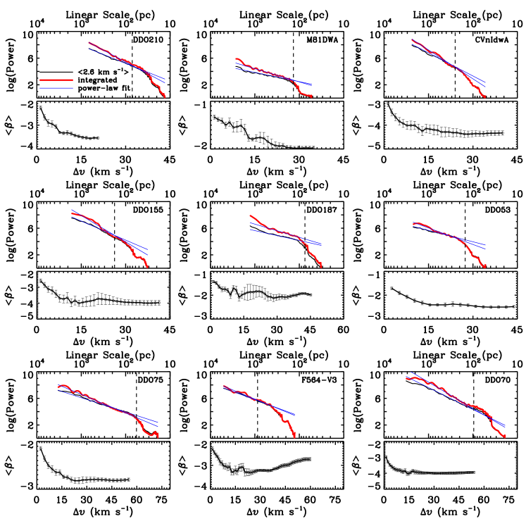
Figure 1.— Power spectrum variations as a function of channel width. The average power spectra of 2.6 km s^-1 thick channel maps (thin black solid line), and power spectra of velocity-integrated maps (thick red solid line) are shown in the upper panel of each galaxy plot. The power-law fit to the power spectrum is overplotted as thin blue solid line. The power spectra have been arbitrarily shifted vertically. The vertical dashed lines mark the linear scales of the synthesized beam. Note that finite size of the synthesized beam causes the decline of power on linear scales smaller than the beam size. Variations of power-law spectral indices with channel width (in velocity units) are shown in the lower panel of each galaxy plot.

Fig. 1–Continued

Fig. 1–Continued

The variations of $<\beta>$ with increasing slice width are shown in Figure 1. The error bars in Figure 1 are determined as the standard deviation of $\beta$ divided by $\sqrt{n}$, where $n$ is the number of slices that were averaged together. In Figure 1, we also present the average power spectra of the 2.6 km s^-1 channel maps (thin black solid lines) and the power spectra of the velocity-integrated maps (thick red solid lines). The vertical dashed lines in Figure 1 mark the linear scales of the synthesized beam. Table 2 lists the linear ranges used in the power-law fitting, the spectral indices of the velocity-integrated and the 1.3 km s^-1 and 2.6 km s^-1 channel maps, the approximate slice width at which the power spectra start getting shallower for smaller slice widths, and the velocity spectral indices, discussed below.

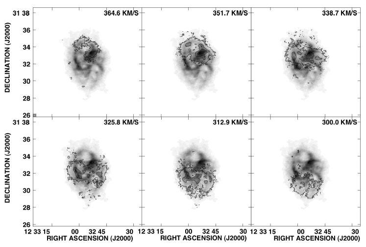
Figure 2.— Every fifth 2.6 km s^-1 channel map of DDO 133 used in our power spectrum analysis is shown as black contours. The grey scale image in each panel is the integrated intensity map. The synthesized beam is indicated at the left-bottom corner of the upper-left panel. The contour levels are 2, 10, and 20 times the rms noise. 

As shown in Figure 1, the power spectra are described very well by a single power law on large scales. Except for the two nearest galaxies (i.e. IC 1613, IC 10), the robust linear scales of the derived power spectra are $\gtrsim$ 100 pc. DDO 187 and F564-V3 have the smallest range (less than a factor of 5) of linear scales used in the power spectrum fitting. As the slice width decreases, the power spectra of F564-V3 and DDO 101 get steeper first, then get shallower. Except for F564-V3 and DDO 101, the others exhibit gradually steeper power spectra as the velocity slice gets thicker, and the spectral index approaches a constant as a significant part of the line profile is integrated together.

The turbulent velocity field is correlated with spatial scales, in the sense that the velocity dispersion on larger scales is usually larger than that on smaller scales. In incompressible turbulence, the turbulent density field passively follows the velocity field. In a narrow channel map, small-scale structures from independent gas elements on the line of sight combine to give relatively more power on smaller scales. This results in a shallower power spectrum for a narrower channel map. However, if the spatially-uncorrelated thermal velocity is non-negligible in a given channel map, then small-scale structures with turbulent velocity dispersions smaller than the thermal speed will lose their distinction. If the thermal velocity is much larger than the turbulent velocity dispersion even on the largest scales, then the thermal velocity component will totally smooth out the spatial correlation present in the turbulent velocity field. Therefore, the shallowing trend for power spectra of narrower channel maps is a reflection of the spatially-correlated turbulent velocity field, modulated by the thermal velocity.

According to the theoretical calculations of LP00, the power-law indices of turbulent density and velocity power spectra can be obtained by changing the width of velocity slices of the PPV data cube. If the effective velocity slice width, which is jointly determined by the instrumental channel width and the thermal velocity (see below), is significantly smaller than the turbulent velocity dispersion on the studied scales, then the velocity slice is regarded to be thin, and the power spectral indices remain constant as the slice width further decreases. If the effective velocity slice width is significantly larger than the turbulent velocity dispersion on the studied scales, then the velocity slice is regarded to be thick, and the power spectral indices remain constant as the slice width further increases. The spectral indices of thick slices are determined solely by the turbulent density fluctuations. In the $\beta$-$\Delta\upsilon$ plot of Figure 1, the asymptote on the side of thick velocity slices suggests that density fluctuations determine the intensity fluctuations there. The shallower power spectra of intensity fluctuations in narrower velocity slices implies more influence from velocity fluctuations.

4. Comparison with a visibility-based estimation of power spectra

Dutta et al. (2009b) have determined H i power spectra of a sample of dwarf galaxies using a different method. They used data from the Giant Metrewave Radio Telescope (GMRT), and the range of baselines roughly corresponds to those of the VLA D and C array configurations. They determined the power spectra directly from the observed visibilities in the $uv$ plane rather than producing maps first and then taking the Fourier Transform and determining the power spectra. This avoids an unnecessary step (converting visibilities into maps) since the $uv$ data are already in the Fourier domain. Here we prefer to identify real emission from the target by working in the image plane. Also, the correction for inclination and primary beam can only be properly done in the image plane.

The Dutta et al. (2009b) study has two galaxies in common with our sample: DDO 210 and DDO 155. They found that DDO 210 has power spectral indices of $-$2.1 $\pm$ 0.6 and $-$2.3 $\pm$ 0.6 for velocity-integrated and single channel (1.7 km s^-1) velocity slices, respectively, and DDO 155 has power spectral indices of $-$0.7 $\pm$ 0.3 and $-$1.1 $\pm$ 0.4 for velocity-integrated and single channel velocity slices, respectively. These are compared to our values of $-$3.66 $\pm$ 0.05 and $-$2.17 $\pm$ 0.09 for DDO 210, and $-$3.97 $\pm$ 0.15 and $-$2.59 $\pm$ 0.12 for DDO 155. Recall that the single channel of 1.3 km s^-1 is narrower than the real velocity resolution of $\sim$ 1.8 km s^-1. The power spectra of DDO 155 are not power-law for linear scales above 1.5 times the beam size, and thus the quality of power-law fitting is very poor (Figure 1). We notice that the power spectra of DDO 155 determined by Dutta et al. (2009b) show similar behavior on large scales. So DDO 155 may not be a good case for comparison. For DDO 210, our single channel spectral index is consistent with that determined by Dutta et al. within the uncertainty of their measurement. Our velocity-integrated spectral index of DDO 210 is much steeper than that determined by Dutta et al. (2009b). Based on figure 8 of Dutta et al. (2009b), the multi-channel-integrated power spectrum of DDO 210 is a very good power law for linear scales above $\sim$ 0.18 kpc, below which the spectrum becomes very noisy and (thus) flat. Dutta et al. included the noisy, flat part of the power spectrum in their power-law fitting, which leads to a much less negative spectral index.

The key difference between the image-domain-based and visibility-based power spectra lies in the different ways used to avoid noise bias. Noise present in the visibilities or images shallows the derived power spectrum. To reduce the effect of noise in the $uv$ plane, Dutta et al. determined the power spectrum by correlating the visibilities at slightly different baselines for which the noise is assumed to be uncorrelated. This method works on the assumption that the angular extent of the galaxy is much smaller than the primary beam of the telescope. The compromise present in this method is that, on the one hand, sufficient visibility pairs are needed to get good statistics and on the other hand, the baseline differences should be as small as possible ($<1/\theta_{0}$, where $\theta_{0}$ is the angular extent of the target galaxy) to have strong enough correlations between visibilities of different baselines.

In the image plane, we distinguish between real emission and noise primarily in two steps. First, in the dirty map, only peaks 2 $\sigma$ above the noise level are regarded as signal and msclean-ed. Second, as described above, only regions with flux $>$ 2 – 3 $\sigma$ in at least three consecutive channels in the smoothed cubes are regarded as real emission, and the rest is blanked. We found that the power spectral indices of both DDO 210 and DDO 155 would be about $-$1.5 regardless of the channel width if we do not apply blanking to the cubes. This implies that non-blanked cubes are predominantly affected by noise on small scales. msclean has been shown to work excellently in recovering extended structures (Cornwell 2008; Rich et al. 2008). Compared to the classical clean, msclean, with its scale-sensitive nature, can clean down to the noise level without leaving skewed noise on the residual map. Furthermore, the recovered fluxes from msclean (and blank) were found to be consistent with those from single-dish observations (Hunter et al., in preparation). Nevertheless, the noise present in the $uv$ data can definitely affect the non-linear deconvolution involved in the image restoration process.

Given these different approximations and assumptions in the two methods, it is not obvious to tell which method is better in determining power spectra. In this work, however, we point out that, 1) by including the deep VLA B-array data, the outer part (longer baseline length) of the $uv$ plane is better sampled in our data; 2) the two galaxies in common all have non-negligible inclinations.

5. Effective velocity slice width and multi-phase neutral H i

The distinction between the thin and thick regimes depends on a comparison between the squared turbulent velocity dispersion on the studied scale $\sigma_{turb,~{}l}^{2}$ and the squared effective velocity slice width $\delta V^{2}$ (LP00)

$$\begin{split}\sigma_{turb,~{}l}^{2}\ll\delta V^{2},~{}{\rm thick}\\ \sigma_{turb,~{}l}^{2}\gg\delta V^{2},~{}{\rm thin}\end{split}$$ (1)

The thermal motion ($v_{T}$), which is spatially incoherent, acts like a smoothing along the velocity dimension. Thermal broadening, together with the instrumental channel width, determine the effective velocity slice width. Assuming a uniform sensitivity across individual channels, the effective velocity slice width is given by

$${\delta V\sim 2(\Delta\upsilon^{2}/6+2v_{T}^{2})^{1/2}}$$ (2)

where $\Delta\upsilon$ and $v_{T}$ are the individual channel width and typical thermal velocity, respectively (LP00). It is the effective velocity slice width, rather than the channel width, that determines the effective slice thickness, and thus the variation of power spectral indices.

The thermal velocity of the gas restricts the minimum effective velocity slice width that can be achieved. For an isothermal gas with temperature $T$, the effective velocity slice width remains nearly constant when the channel width becomes smaller than the thermal velocity $v_{T}$ ($\sqrt{2k_{\rm B}T/m\pi}$), and thus the power spectral indices do not change. Empirically, the median channel width at the point where the power spectra start to get shallower for narrower channel width is $\sim$ 15 km s^-1 for our sample galaxies (Table 2). A two-phase (WNM and CNM) description of the neutral H i was suggested by Field, Goldsmith, & Habing (1969). Wolfire et al. (2003) demonstrate that the interstellar H i at a temperature of $\sim$ 100 K and of $\sim$ 8000 K can coexist in thermal equilibrium. Therefore, if there is only thermally stable WNM, the power spectral indices would not change for channel widths narrower than $\sim$ 6.5 km s^-1 (the thermal velocity of H i gas with a temperature of 8000 K). For the thirteen galaxies with a channel width of 1.3 km s^-1, the power spectra keep getting shallower for narrower channel width, down to 1.3 km s^-1. This suggests widespread H i with a temperature $\sim$ 600 K (corresponds to a thermal velocity of 1.8 km s^-1) or even lower, considering that the real velocity resolution is 1.8 km s^-1. In the Milky Way, Heiles & Troland (2003) found that more than 48% of the WNM, which accounts for $\sim$ 60% of the total H i, is in the thermally unstable regime with a broad temperature range from $\sim$ 500 – 5000 K. A temperature of $\sim$ 600 K lies in the broad boundary between the WNM and CNM.

The typical velocity dispersion from H i emission line observations of nearby star-forming galaxies is $\sim$ 10 km s^-1 (e.g. Côté, Carignan & Freeman 2000; Leroy et al. 2008), which is the combination of turbulent and thermal velocity dispersions. Therefore, $\sim$ 10 km s^-1 can be regarded as an upper limit on the turbulent velocity on galactic scales. Also, since the maximum temperature $T_{\rm max}$ of neutral H i is $\sim$ 10⁴ K, the minimum possible turbulent velocity dispersion $\sigma_{turb}$ should be $\sim$ 4 km s^-1 ($\sqrt{10^{2}-v_{T_{\rm max}}^{2}}$). For a given scale, the thin (thick) regime is reached if the squared effective slice width is much smaller (larger) than the squared turbulent velocity dispersion (Inequality 1). In the $\beta$ vs. $\Delta\upsilon$ plot, two asymptotes are expected for the two regimes of thin and thick effective velocity slices. As mentioned above, the H i gas with a temperature of $\sim$ 600 K has a thermal velocity $v_{T}$ $\sim$ 1.8 km s^-1 which is the highest spectral resolution for our data. With $v_{T}$ = 1.8 km s^-1 and $\Delta\upsilon$ = 1.8 km s^-1, Equation 2 gives an effective velocity slice width of $\sim$ 5 km s^-1. Since we do not see the asymptotic behavior towards the single channel width in the $\beta$ vs. $\Delta\upsilon$ plot (Figure 1), the single channel, and thus the effective velocity slice width of 5 km s^-1 does not reach the thin regime, at lease for the thermally unstable WNM components with a temperature $\lesssim$ 600 K. Based on Inequality 1, the turbulent velocity dispersion $\sigma_{turb,~{}l}$ for the neutral H i gas with a temperature $\lesssim$ 600 K is not much higher (i.e. by less than a factor of 3) than $\sim$ 5 km s^-1, which is mildly supersonic.

The line profiles of our galaxies cover a velocity range from $\sim$ 20 to 130 km s^-1. The velocity-integrated slices lie in the thick slice regime, as implied by the asymptotes seen in Figure 1. As mentioned above, our galaxies start reaching the thick regime at a channel width of $\sim$ 15 km s^-1 on average. With $v_{T}$ = 6.5 km s^-1 ($T_{\rm WNM,stable}$ = 8000 K) and $\Delta\upsilon$ = 15 km s^-1, Equation 2 gives an effective velocity slice width of 22 km s^-1. Therefore, to be in the thick regime defined in Inequality 1, the turbulent velocity dispersion of the thermally stable WNM should be much smaller (i.e. by at least a factor of 3) than 22 km s^-1. Therefore, the maximum Mach number for the thermally stable WNM components should be smaller than $\sim$ 1 ($\sigma_{turb,~{}l}$/$v_{T_{\rm WNM,stable}}$, $\sigma_{turb,~{}l}$ $<$ 22/3).

The intensity fluctuations of the velocity-integrated maps are determined by density fluctuations including all possible phases of H i. On the other hand, as explained above, the shallowing trend for power spectra of channel maps narrower than 6.5 km s^-1 is only caused by turbulent velocity fluctuations of cooler H i, including the thermally unstable components and (possibly) some CNM. The large H i self-absorption survey by Gibson et al. (2005) found a smoothly distributed, albeit fluffy, cold phase of H i in the Milky Way Galaxy, which is in line with our finding that H i gas with a temperature of 600 K or even lower is widespread in dIrr galaxies.

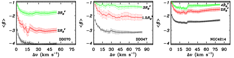
Figure 3.— Variations of 1D spectral indices as a function of channel width for three galaxies. The red triangles denote the spectral indices of azimuthal scans at an inner radius, measured in units of $V$-band disk scalelength. The green upside down triangles denote the spectral indices of azimuthal scans at an outer radius. The 2D spectral indices presented in Figure 1 are shown as black circles. 

Zhang et al. (2012) found that star-forming disks of most local dIrr galaxies have been shrinking at least during the past $\sim$ Gyr. Cold atomic gas is the precursor to molecular cloud formation which shows an almost linear correlation with the SFR in nearby star-forming galaxies (e.g. Leroy et al. 2008). Possible radial variations of the $\beta$-$\Delta\upsilon$ relation would reflect the relative spatial distributions of H i gas with different temperatures. We took one-dimensional (1D) power spectra of azimuthal scans at different radii (e.g. Elmegreen et al. 2003) for our galaxies. Figure 3 presents the results for three of our galaxies (DDO 70, DDO 47 and NGC 4214). The 1D power spectra in Figure 3 are the average of adjacent azimuthal scans with a radial extent of two synthesized beams. We used the same geometric parameters derived above for the extraction of azimuthal profiles. The black symbols correspond to the 2D power spectra as shown in Figure 1. The red and green symbols, respectively, denote the spectral indices at inner and outer radii, in units of the $V$-band disk scalelength $R_{D}^{V}$. In an isotropic field, the 1D power spectra of azimuthal profiles are expected to be shallower than the 2D power spectra by $\sim$ 1 because of the reduced dimension (see the power spectra of inner radii in Figure 3). The azimuthal scans at the outer radii have systematically shallower power spectra than those at the inner radii, which may signify a gradual change from 3D to 2D geometry, possibly due to the longer azimuthal scans at the outer radii. Obviously, the inner regions exhibit a much stronger shallowing trend toward narrower channel width. This suggests that the shallowing trend observed for the 2D power spectra, and thus the structure associated with the cooler H i, is dominantly contributed by the inner, more actively star-forming regions. The more widespread cool H i in the inner disk may be caused by a higher mid-plane gas pressure (Wong & Blitz 2002; Blitz & Rosolowsky 2004) or a higher average gas volume density (Gao & Solomon 2004) there. Braun (1997) studied the neutral H i properties of a sample of 11 nearby spiral galaxies. He found positive radial gradients of the H i kinematic temperature, and that there are more H i components with narrow ($\lesssim$ 6 km s^-1) emission line profiles in the inner disks.

6. Power spectral index vs. SF

The ISM structure in dIrr galaxies can be significantly influenced by stellar feedback. Shells and holes of up to $\sim$ kpc scales are often seen in the H i gas distribution of dwarf galaxies (e.g. Sargent et al. 1983; Puche et al. 1992; Young & Lo 1997; Walter & Brinks 1999; Ott et al. 2001; Muller et al. 2003; Simpson, Hunter & Knezek 2005; Cannon et al. 2011). It has been shown that stellar feedback can provide sufficient energy to produce the observed shells and holes (Warren et al. 2011).  Stellar energy, such as winds, ionizing radiation, and supernova explosions, dominates the energy injection into the ISM (Mac Low & Klessen 2004) on the corresponding scales, at least in star-forming galaxies. By studying the visibility-based power spectra of seven dwarf galaxies, Dutta et al. (2009b) found that the galaxies with higher SFR surface density tend to have steeper H i power spectra, implying more large-scale structures of H i for more intense SF. With a much larger sample, we can explore the possible relationship between the power spectra and SF.

For most of the galaxies (Table 2), the minimum linear scales covered by our power spectra are $\gtrsim$ 100 pc, which is probably comparable with the expected disk scale height of dIrr galaxies (e.g. van den Bergh 1988; Staveley-Smith et al. 1992; Carignan & Purton 1998; Elmegreen, Kim & Staveley-Smith 2001; Banerjee et al. 2011). A break in the power-law power spectrum of the H i emission distribution has been observed for a few galaxies (LMC – Elmegreen et al. 2001; NGC 1058 – Dutta et al. 2009a). The power spectral index for smaller scales (compared to the break scale) is steeper than for larger scales by $\sim$ 1, which is found both in the LMC (Elmegreen et al. 2001) and simulations of gas-rich galaxies (Bournaud et al. 2010). The flattening of the power spectrum on larger scales is understood as the transition from isotropic 3D turbulence on smaller scales to anisotropic 2D turbulence on larger scales (Bournaud et al. 2010). The break is about the gas disk scale height (Elmegreen et al. 2001; Bournaud et al. 2010).

Figure 4.— The synthesized beam size (pc) is plotted against the velocity-integrated power spectral indices determined by fitting a linear scale range from 1 to 1.5 times the beam size. 

As described in Section 3, we did power law fitting to the power spectra for linear scales larger than 1.5 times the synthesized beam. This is because the finite size of the synthesized beam results in a pronounced decline at high spatial frequencies of the power spectra (Figure 1). Nevertheless, we expect the power spectra at high spatial frequencies, although being noticeably influenced by the beam, still partially reflect the intrinsic power spectra of the galaxy at the resolution limit. Figure 4 presents the relation between the beam size (in units of pc) and the velocity-integrated power spectra fitted over linear scales from 1 to 1.5 times the beam size. Our galaxies fall into two groups in Figure 4, separated around a beam size of $\sim$ 200 – 300 pc, below which the galaxies have more negative indices. The two groups are also roughly divided by a spectral index of $-$3. This may reflect the effect of the disk thickness, because anisotropic 2D turbulence on large scales is expected to have much shallower power spectra than isotropic 3D turbulence on small scales.

The SMC, which is like the most luminous galaxies in our sample in terms of stellar and gas masses, does not have a break in the power spectrum between linear scales of 30 pc and 4 kpc (Stanimirović et al. 1999). This lack of a break indicates that the maximum transverse scale is comparable to or smaller than the H i line-of-sight depth. Perhaps the 3D behavior of the power spectrum of the SMC across a large range of linear scales is a result of the tidal interaction with the LMC during the past few Gyr. The numerical simulations by Bekki & Chiba (2007) found that almost 20% of the SMC’s gas may have been accreted by the LMC during their recent interaction, and this may explain the origin of the LMC’s intermediate-age stellar populations with distinctively low metallicities (e.g. Geisler et al. 2003). So it is possible that the SMC’s gas disk may have been stretched during the recent interaction, resulting in a thicker disk. For the two nearest galaxies in our sample, IC 10 and IC 1613, the power spectra also can be well fitted with a single power law between linear scales of $\sim$ 50 pc and $\sim$ 2 kpc. IC 1613 has a tidal index $\sim$ 0.9 (Karachentsev et al. 2004), which indicates that this galaxy has been significantly influenced by the neighboring galaxies (e.g. M 33). Our H i kinematics analysis (Oh et al. in preparation) suggests that these two galaxies, and also the very low luminosity galaxies, such as DDO 210 and DDO 155, have ratios of the maximum rotational velocity to velocity dispersion $\lesssim$ 2, which indicates that the gas distribution may be a relatively thick disk or even triaxial ellipsoid. We note that, Roychowdhury et al. (2010, see also Sánchez-Janssen et al. 2010) found a mean intrinsic axial ratio of $\sim$ 0.6 for the H i disks of dIrr galaxies with $M_{B}$ $>$ $-$14.5 mag, which suggests very thick gas disks in faint dIrr galaxies.

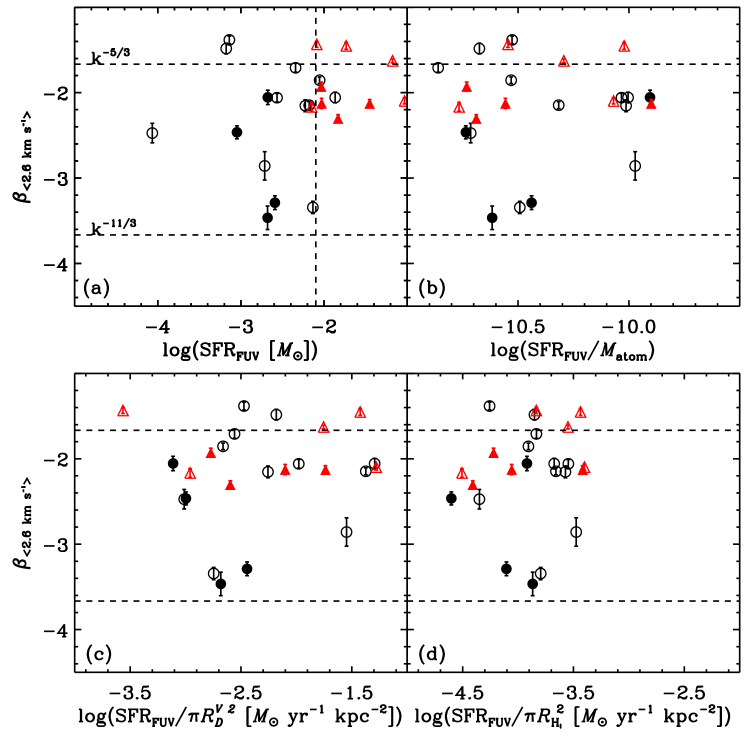
Figure 5.— Power spectral indices of 2.6 km s^-1 channel maps are plotted against the SFR determined from the FUV (a), SF efficiency (b), SFR normalized by the area enclosed by the radius of one $V$-band disk scale length (c), and SFR normalized by the area enclosed by the radius where the H i column density falls off to 10¹⁹ cm^-2 (d). The open and filled symbols respectively denote the galaxies with spectral indices measured at high spatial frequencies (linear scales between 1 and 1.5 times the beam size) more negative and less negative than $-$3. The black circles and red triangles respectively denote the galaxies with $M_{B}$ $>$ $-$14.5 mag and $M_{B}$ $<$ $-$14.5 mag. The horizontal dashed lines mark the expected 1D ($P\sim k^{-5/3}$) and 3D ($P\sim k^{-11/3}$) power spectral indices of a Kolmogorov-type turbulence. The vertical dashed line in panel (a) marks the division (log(SFR_FUV) = $-$2.1) of the bimodality discussed in the text. We notice that there is a slight trend for the galaxies with $M_{B}$ $<$ $-$14.5 mag in panel (d), in the sense that higher SFR surface density corresponds to shallower power spectra, but the scatter is too large to be sure.

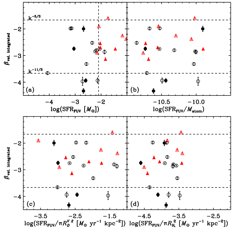
Figure 6.— Same as Figure 5 but for velocity-integrated maps. The slight correlation found in Figure 5d is also present here in panel (d).

Figures 5 and 6 plot the power spectral indices against SF-related quantities derived from the far-UV (FUV, SFR_FUV): SF efficiency of the atomic gas (SFR_FUV/$M_{\rm atom}$), SFR surface density normalized to the area within one $V$-band disk scalelength (SFR/$\pi{{R_{D}^{V}}^{2}}$), and SFR surface density within the radius where the H i column density falls off to $10^{19}$ cm^-2(SFR/$\pi$${\it R}_{\rm H\textsc{i}}$²), for 1.3 and 2.6 km s^-1 thick slices and for the velocity-integrated maps, respectively. For the formula used to derive SFR_FUV from the FUV, the reader is referred to Hunter et al. (2010) and Zhang et al. (2012). The total atomic gas mass $M_{\rm atom}$ (1.34$\times$ $M_{\rm H\textsc{i}}$ to account for He) used here was collected from single-dish observations in the literature (see Hunter & Elmegreen 2004 for the references). The open and filled symbols respectively denote the galaxies with spectral indices measured at high spatial frequencies (1–1.5 times the beam) more negative and less negative than $-$3, i.e. the two groups mentioned above. The black circles and red triangles respectively denote the galaxies with $M_{B}$ $>$ $-$14.5 mag and $M_{B}$ $<$ $-$14.5 mag. There is no strong correlation in these plots. However, Figure 5 suggests that all the galaxies with log(SFR) $>$ $-$2.1 have narrow channel spectral indices around $-$2, whereas galaxies with lower SFR exhibit a much larger scatter toward more negative spectral indices. The vertical dashed line in panel (a) of Figure 5 marks the division at log(SFR) = $-$2.1. Similarly, in Figure 6, the spectral indices of velocity-integrated maps exhibit a larger scatter (toward more negative indices) in galaxies with lower SFR.

Figure 7.— Power spectral indices of 2.6 km s^-1 channel maps ($left~{}panel$) and velocity-integrated maps ($right~{}panel$) are plotted against $B$-band absolute magnitude $M_{B}$. The open and filled symbols respectively denote the galaxies with spectral indices measured at high spatial frequencies (linear scales between 1 and 1.5 times the beam size) more negative and less negative than $-$3. The horizontal dashed lines mark the expected 1D ($P\sim k^{-5/3}$) and 3D ($P\sim k^{-11/3}$) power spectral indices of a Kolmogorov-type turbulence. The vertical dashed lines mark the division of the bimodality ($M_{B}$ = $-$14.5 mag) discussed in the text.

Given that the spectral indices show the bimodality with the SFR but not the SFR surface density, the bimodality may just reflect the correlation between spectral indices and the mass (or size) of galaxies. In Figure 7, the spectral indices of 2.6 km s^-1 channel maps and spectral indices of velocity-integrated maps are plotted against $B$-band absolute magnitude $M_{B}$. There exists a similar bimodality as that present between power spectral indices and the SFR. The vertical dashed lines in Figure 7 mark the division of the bimodality at $M_{B}$ = $-$14.5 mag. Brighter galaxies tend to have flatter power spectra. This could be a result of disk thickness, in the sense that brighter galaxies tend to have a higher ratio of radial length to thickness, and so are more 2D on average. The three galaxies which have the most negative spectral indices (for both narrow channel maps and velocity-integrated maps) are CVnIdwA, DDO 70 and DDO 133. The negative tidal indices of these three galaxies (Karachentsev et al. 2004) suggest that they do not have significant interactions with neighboring galaxies.

This ratio of radial length to thickness also affects the regularity of galactic structure because the thickness is approximately the turbulent Jeans length, and therefore the typical size for stellar complexes. When the radial length is large compared to the thickness, there is room in the disk for a lot of star-forming clumps, giving the disk a somewhat uniform appearance. But when the radial length is small compared to the thickness, there may be only a few star-forming complexes with large stochasticity, which can lead to an irregular appearance of the disk. Thus the correlation we find between the slope of the power spectrum and the galaxy absolute magnitude (or total SFR) may explain the findings of Lee et al. (2007), who explored the distribution of the Local Volume galaxies in the $M_{B}$-H$\alpha$ equivalent width plane. They found a bimodality around $M_{B}\sim$ $-$15 mag in the sense that galaxies with lower luminosity exhibit a larger (by a factor of 2) scatter in H$\alpha$ equivalent width than galaxies with higher luminosity ($-$19 $\lesssim M_{B}\lesssim$ $-$15 mag).

The lack of a strong correlation between the inertial range spectral indices and SFR surface density (and also SF efficiency) may be unsurprising. In the classical Kolmogorov turbulence, the energy transfer occurs locally (cascade) in the wavenumber space in the inertial range, and the driving only affects the energy input at the top of the cascade. Unlike this ideal Kolmogorov turbulence which has a single driving source on the large scale, the driving of turbulence in the ISM may span a wide range of scales. The stellar energy can drive turbulence from parsec-scale supernovae up to hundred-parsec-scale superbubbles (Mac Low & Klessen 2004). Similarly, gravitational energy may feed the turbulence through sub-parsec gravitational collapse, up to galactic-scale gravitational instabilities (e.g. Wada et al. 2002; Elmegreen et al. 2003; Agertz et al. 2009) and galaxy interactions (e.g. Elmegreen & Scalo 2004), etc. Therefore, the single power-law behavior of H i power spectra suggests that the turbulence may be driven (by whatever energy sources) over a wide range of physical scales, otherwise the power spectra should exhibit features, such as a flattening at low wavenumbers, at the primary driving scale (e.g. Nakamura & Li 2007; Padoan et al. 2009). Supernovae are the largest contributers of energy input to the ISM on scales comparable to or smaller than the disk thickness (Mac Low & Klessen 2004). However, it was suggested that supernova driven turbulence alone cannot explain the broad H i emission lines, at least in the outer parts of disk galaxies (e.g. Dib, Bell & Burkert 2006; Tamburro et al. 2009). Furthermore, simulations (e.g. Agertz et al. 2009; Bournaud et al. 2010) found that gravitational instabilities alone can reproduce the observed power-law power spectra, the stellar feedback does not significantly change the ISM statistical properties established by gravitational instabilities. In addition, the multi-phase nature of the ISM implies that thermal instabilities (e.g. Field 1965) may also be an important driving agent of turbulence (e.g. Hennebelle & Audit 2007; Gazol & Kim 2010). Thus turbulence may be driven by many sources and the properties of this turbulence on scales smaller than the sources may be independent of these sources, so a correlation between spectral index and SFR surface density might not be expected.

The slope of the power spectrum may depend on the nature of the driving force (no matter whether it is stellar or non-stellar). Recent simulations done by Federrath, Klessen, & Schmidt (2009) suggest that, at a given Mach number, compressive forcing can lead to steeper density spectra than solenoidal forcing (rotational, incompressible). Kim & Ryu (2005), Kowal, Lazarian, & Beresnyak (2007), and Gazol & Kim (2010) found a correlation between power spectral index and Mach number from magnetohydrodynamic (MHD) simulations, in the sense that higher sonic Mach number leads to shallower density power spectra. This correlation was interpreted as the result of more small-scale density structures generated by stronger shocks in supersonic flows. In the present observations, the lack of a correlation between the power spectral indices and the SFR surface density may imply that stellar feedback and other energy sources share similar characteristics of driving on average. Burkhart et al. (2010) also found little correlation between SF activity and Mach number in a 2D map based on kurtosis of H i line profiles in the SMC. They found that regions with the highest sonic Mach number lie around the bar. Chappell & Scalo (2001) arrived at a similar conclusion using a multifractal spectrum analysis of low-mass star-forming cloud complexes: there is little correlation between the geometrical properties of the gas and the level of internal SF.

As we discussed above, higher-luminosity galaxies ($M_{B}$ $<$ $-$14.5 mag) in our sample may have 2D turbulence on the studied scales and 3D turbulence on unresolved scales, whereas lower-luminosity galaxies may have only 3D turbulence because the disks are thick relative to their radial length scales. Therefore, it may be desirable to explore the relationship between SFR surface density and power spectral indices for higher-luminosity and lower-luminosity galaxies separately. Figures 5 and 6 suggest that our claim of a lack of a correlation between SFR surface density and spectral indices is valid for galaxies with both $M_{B}$ $<$ $-$14.5 mag or $M_{B}$ $>$ $-$14.5 mag. The lack of a correlation for the more luminous galaxies makes sense according to the above discussion if their power spectra are dominated by 2D turbulence and stellar feedback has little effect on scales larger than the disk thickness. The lack of a correlation for less luminous galaxies, which have relatively thicker disks than more luminous galaxies, suggests that local SF does not strongly affect the spectral index of turbulence.

7. The turbulent velocity field

Unlike the spectra that reflect density fluctuations, velocity spectra (specific kinetic energy spectra) are directly related to the turbulent energy distribution across different scales. Intensity fluctuations within channel maps are contributed by both the density and velocity fields. However, the relevant importance of density and velocity fields changes with the amplitude of the density fluctuations. For example, intensity fluctuations simply follow the velocity field if the density field is constant. Our thick velocity slices, especially the velocity-integrated ones, have intensity fluctuations dominated by variations in the density field. According to LP00, the spectral index of (2D) thick velocity slices $\beta_{\rm thick}$ (e.g. $\beta_{\rm integrated}$ listed in Table 2) is equal to the 3D density spectral index $\beta_{\rm density}$, provided the maximum transverse scale is comparable to or smaller than the line-of-sight depth. In an isotropic 3D turbulent medium, if the density spectral index $<-3$, the velocity spectral index $\beta_{\rm velocity}$ is equal to $-2\beta_{\rm thin}-9$, where $\beta_{\rm thin}$ is the spectral index of intensity fluctuations within thin velocity slices. $\beta_{\rm velocity}$ is equal to $-3-2(\beta_{\rm thin}-\beta_{\rm thick})$ if the density spectral index $>-3$.

As discussed in Section 4, the velocity resolution of 2.6 km s^-1 does not yet reach the thin slice regime. Assuming the 2.6 km s^-1 velocity slice is thin (i.e. $\beta_{\rm thin}$ = $\beta_{\rm 2.6}$) and the line-of-sight depth is comparable to the maximum transverse scale we studied, we can obtain the velocity spectral indices $\beta_{\rm velocity}$ which are listed in Table 2. Sixteen galaxies have velocity power spectra steeper than that of Kolmogorov turbulence (for which $\beta_{\rm velocity}$ would be $-$11/3 for 3D turbulence). The real velocity spectral indices can be even steeper because we do not yet reach the “thin” regime. If the line-of-sight depth is smaller than the maximum transverse scale, the measured $\beta_{\rm thick}$ and $\beta_{\rm thin}$ should be subtracted by $\sim$ 1 to be used for the calculation of $\beta_{\rm density}$ and $\beta_{\rm velocity}$, and thus the resultant $\beta_{\rm density}$ would be $\beta_{\rm thick}$ $-$ 1, and $\beta_{\rm velocity}$ would be shallower than those listed in Table 2 by $\sim$ 2 when the $\beta_{\rm density}$ $<$ $-$3, whereas $\beta_{\rm velocity}$ determined for the galaxies with $\beta_{\rm density}>-$ 3 is not affected (see the relations in the preceding paragraph). We point out that, if the steepening factor of 2D turbulence relative to 3D turbulence is not 1, then we would not know how to obtain $\beta_{\rm density}$, and, in the case of $\beta_{\rm thick}$ $<$ $-$3, $\beta_{\rm velocity}$ when the line-of-sight depth is smaller than the maximum transverse scales.

MHD isothermal simulations (e.g. Kritsuk et al. 2007; Federrath et al. 2009; Gazol & Kim 2010) suggest that fluids with higher Mach number (thus stronger compressibility) have steeper velocity power spectra (and shallower density power spectra). However, the isothermal assumption adopted in most simulations may not be valid for the multi-phase H i for which thermal instabilities can be an important driving mechanism of turbulence (Hennebelle & Audit 2007; Gazol & Kim 2010). We emphasize that the multi-phase nature of the H i makes the velocity spectral indices derived here questionable, because the density power spectra determined from thick velocity slices may invoke density fields of all different phases of H i, whereas the turbulent velocity fields as reflected by the shallower power spectra within narrower velocity slices only include contributions from the thermally unstable WNM and (possibly) some CNM.

8. Summary

We have studied the H i power spectral index variations with channel width for a sample of nearby dIrr galaxies. The majority of the 2D power spectra cover more than one decade of linear scales, from $\sim$ hundred pc to several kpc. The main results are summarized as follows.

1. The power spectral indices asymptotically become a constant for each galaxy when a significant part of the line profile is integrated, consistent with the theoretical calculations of LP00. This indicates that density fluctuations, including all possible temperature components of H i, determine the intensity fluctuations of our “thick” velocity slices.

2. Starting at a channel width of $\sim$ 15 km s^-1 on average for our sample, narrower channel maps have shallower power spectra. The shallowing trend, which is caused in part by turbulent velocity dispersions of the thermally unstable WNM and possibly some CNM, continues down to the single channel maps (1.3 km s^-1). This continuation indicates that, first, even the highest velocity resolution of 1.8 km s^-1 is not smaller than the thermal dispersion of the coolest H i ($\lesssim$ 600 K) which is widespread in our galaxies; if it were, then the spectral index would remain constant. Second, the turbulent velocity dispersion of the coolest H i ($\lesssim$ 600 K) probed at our highest velocity resolution is not much larger than $\sim$ 5 km s^-1, which means that the turbulence in this phase of H i is mildly supersonic.

3. Toward narrower channel width, the 1D power spectra of azimuthal profiles at the inner radii have a stronger shallowing trend than those at the outer radii, which implies that the shallower power spectra for narrower channel maps are mainly contributed by the inner disks, and thus the inner, more actively star-forming regions have proportionally more cooler H i than the outer regions.

4. The power spectra of IC 1613 and IC 10, which are the two nearest galaxies in our sample, can be well fitted with a single power law between linear scales of $\sim$ 50 pc and $\sim$ 2 kpc. This suggests that the H i line-of-sight depth may be comparable with the maximum transverse scales in these two galaxies.

5. Our sample galaxies exhibit a bimodality in the spectral indices versus $M_{B}$ (and also SFR) plane. The division of the bimodality is at $M_{B}\sim$ $-$14.5 mag and log(SFR ($M_{\odot}\;{\rm yr}^{-1}$)) $\sim$ $-$2.1. Galaxies with higher luminosity and SFR tend to have shallower power spectra with a smaller scatter, whereas galaxies with lower luminosity and SFR exhibit a much larger scatter toward more negative spectral indices. The bimodality may signify that higher-luminosity galaxies tend to have bigger gas disks compared to their thicknesses, whereas lower-luminosity galaxies may be better described as thick disks or even triaxial ellipsoids.

6. The inertial range spectral indices of single channel maps and velocity-integrated maps are not correlated with the SFR surface density. This may imply that either stellar and non-stellar energy sources can excite turbulence with about the same power spectral index, or non-stellar energy sources are more important in driving ISM turbulence. The single power-law behavior of the power spectra indicates that the ISM turbulence may be driven, from whatever energy sources (stellar or non-stellar), over a wide range of physical scales, otherwise we should see features, such as a flattening of power spectra at low wavenumbers, at the primary driving scale.

The multi-phase (i.e. different temperature components) nature of galactic neutral H i means that the power spectra determined for different velocity slice widths trace different temperature components of H i. Therefore, determining the turbulent velocity spectral indices may be difficult, and more theoretical work taking into account the multi-phase nature of neutral H i is needed.

Table 1Galaxy Sample

Galaxy	Other Names	D	MB	log(SFR)	log(M${}_{\rm atomic~{}gas}$)	${\it R}_{\rm H\textsc{i}}$	$R_{D}^{V}$	Incl.
		(Mpc)	(mag)	($M_{\odot}$ yr-1)	($M_{\odot}$)	(kpc)	(kpc)	(degrees)
(1)	(2)	(3)	(4)	(5)	(6)	(7)	(8)	(9)
DDO 210	Aquarius Dwarf	0.9	$-$10.38	$-$4.07	6.52	0.78	0.17	47
M81dwA	KDG 052	3.6	$-$11.46	$-$3.14	7.26	2.04	0.26	0
CVnIdwA	UGCA 292	3.6	$-$12.16	$-$2.68	7.81	2.22	0.57	41
DDO 155	UGC 8091, GR 8	2.2	$-$12.25	$-$2.71	7.13	1.35	0.15	48
DDO 187	UGC 9128	2.2	$-$12.38	$-$3.14	7.37	1.23	0.18	32
DDO 53	UGC 4459, VIIZw 238	3.6	$-$13.43	$-$2.34	8.39	3.14	0.72	43
DDO 75	UGCA 205, Sextans A	1.3	$-$13.72	$-$2.18	8.01	3.09	0.22	34
F564-V3	LSBC D564-08	8.7	$-$13.67	$-$3.05	7.56	3.37	0.53	53
DDO 70	UGC 5373, Sextans B	1.3	$-$13.74	$-$2.59	7.72	3.22	0.48	24
NGC 4163	UGC 7199	2.9	$-$13.95	$-$1.73	7.34	0.60	0.10	0
IC 1613	UGC 668, DDO 8	0.7	$-$14.17	$-$2.23	7.66	2.66	0.58	38
Haro 29	UGCA 281, Mrk 209, IZw 36	5.9	$-$14.39	$-$1.87	8.01	4.52	0.29	42
DDO 46	UGC 3966	6.1	$-$14.36	$-$2.05	8.35	4.76	1.14	29
DDO 133	UGC 7698	3.5	$-$14.36	$-$2.13	8.23	3.82	1.14	43
DDO 63	UGC 5139, Holmberg I	3.9	$-$14.58	$-$2.09	8.33	4.22	3.09	0
DDO 87	UGC 5918, KDG 072, VIIZw 347	7.7	$-$14.52	$-$2.15	8.49	8.51	1.43	28
DDO 101	UGC 6900	6.4	$-$14.40	$-$2.68	7.10	2.36	0.93	49
DDO 43	UGC 3860	7.8	$-$14.75	$-$2.03	8.40	5.82	0.61	46
DDO 52	UGC 4426	10.3	$-$15.05	$-$2.03	8.57	6.99	1.32	53
DDO 47	UGC 3974	5.2	$-$15.17	$-$1.83	8.73	10.97	1.36	19
IC 10	UGC 192	0.7	$-$15.75	$-$1.73	8.16	4.00	0.40	41
DDO 50	UGC 4305, Holmberg II	3.4	$-$16.39	$-$1.18	8.99	8.67	1.10	47
NGC 3738	UGC 6565, Arp 234	4.9	$-$16.70	$-$1.45	8.32	5.42	0.78	46
NGC 4214	UGC 7278	3.0	$-$17.26	$-$1.03	8.91	8.62	0.75	26

Note. — (1) Galaxy name. (2) The other commonly used names in the literature. (3) Distance from D. A. Hunter et al. (2012, in preparation and references therein). (4) $B$-band absolute magnitude. (5) Logarithm of SFR derived from the FUV luminosity (Hunter et al. 2010; Zhang et al. 2012). (6) Logarithm of the atomic gas mass (1.34$\times$$M_{\rm H\textsc{i}}$) is collected from single-dish observations in the literature (see Hunter & Elmegreen 2004 for the references). (7) The radius where the H i column density falls off to 10¹⁹ cm^-2. (8) Disk scale length measured on the $V$-band images. (9) The inclination angles derived by fitting the iso-intensity contours on the velocity-integrated H i maps.

Table 2Power Spectra

Galaxy	Minscale	Maxscale	$<\beta_{\tt 1.3}>$	$\sigma_{\beta}$	$<\beta_{\tt 2.6}>$	$\sigma_{\beta}$	$\beta_{\tt integrated}$	$\sigma_{\beta}$	Chchange	$\beta_{\tt velocity}$
	(kpc)	(kpc)							(km s-1)
(1)	(2)	(3)	(4)	(5)	(6)	(7)	(8)	(9)	(10)	(11)
DDO 210	0.11	0.68	$-$2.17	0.09	$-$2.47	0.11	$-$3.66	0.05	15	$-$4.05
M81DWA	0.20	1.35	$-$1.33	0.04	$-$1.38	0.04	$-$1.98	0.04	27	$-$4.19
CVnIdwA	0.38	2.37	$-$3.09	0.13	$-$3.47	0.14	$-$4.33	0.09	23	$-$2.07
DDO 155	0.27	1.65	$-$2.59	0.12	$-$2.86	0.16	$-$3.97	0.15	6	$-$3.28
DDO 187	0.11	0.43	$-$1.43	0.05	$-$1.48	0.06	$-$1.98	0.04	9	$-$4.00
DDO 53	0.23	2.23	$\cdots$	$\cdots$	$-$1.71	0.05	$-$2.48	0.04	15	$-$4.54
DDO 75	0.09	1.67	$\cdots$	$\cdots$	$-$2.15	0.04	$-$2.80	0.03	23	$-$4.31
F564-V3	1.31	5.09	$-$2.30	0.08	$-$2.46	0.08	$-$2.74	0.07	9	$-$3.56
DDO 70	0.14	1.61	$-$2.97	0.06	$-$3.29	0.08	$-$3.94	0.07	12	$-$2.42
NGC 4163	0.16	2.54	$-$1.73	0.04	$-$2.06	0.05	$-$3.32	0.04	24	$-$4.88
IC 1613	0.05	2.37	$\cdots$	$\cdots$	$-$2.15	0.07	$-$2.85	0.02	26	$-$4.38
Haro 29	0.39	2.07	$-$1.80	0.05	$-$2.06	0.06	$-$2.87	0.07	17	$-$4.62
DDO 46	0.32	2.29	$-$1.59	0.04	$-$1.85	0.04	$-$2.75	0.02	14	$-$4.80
DDO 133	0.43	4.61	$\cdots$	$\cdots$	$-$3.34	0.07	$-$3.94	0.10	13	$-$2.31
DDO 63	0.22	2.05	$\cdots$	$\cdots$	$-$1.44	0.04	$-$1.90	0.03	28	$-$3.93
DDO 87	0.48	4.50	$\cdots$	$\cdots$	$-$2.17	0.05	$-$2.90	0.03	15	$-$4.46
DDO 101	0.59	3.06	$\cdots$	$\cdots$	$-$2.05	0.08	$-$2.00	0.10	10	$-$2.88
DDO 43	0.65	5.87	$\cdots$	$\cdots$	$-$2.13	0.06	$-$2.56	0.06	13	$-$3.86
DDO 52	0.85	4.93	$-$1.59	0.05	$-$1.93	0.05	$-$2.54	0.05	14	$-$4.23
DDO 47	0.42	3.91	$\cdots$	$\cdots$	$-$2.30	0.05	$-$3.14	0.05	21	$-$4.39
IC 10	0.04	2.46	$\cdots$	$\cdots$	$-$1.45	0.04	$-$1.59	0.02	13	$-$3.28
DDO 50	0.25	2.72	$\cdots$	$\cdots$	$-$1.63	0.02	$-$2.25	0.02	26	$-$4.25
NGC 3738	0.32	3.04	$-$1.82	0.04	$-$2.13	0.05	$-$2.75	0.04	13	$-$4.24
NGC 4214	0.18	9.26	$-$1.92	0.03	$-$2.10	0.03	$-$2.31	0.05	14	$-$3.43

Note. — (1) Galaxy name. (2) The minimum linear scale in the power-law fitting to the power spectra. Min_scale is equal to 1.5 times the beam size. (3) The maximum linear scale in the power-law fitting to the power spectra. (4) The average 2D power spectral index of the 1.3 km s^-1 velocity slices. (5) The uncertainty of the power spectral index of the 1.3 km s^-1 velocity slices. (6) The average power spectral index of the 2.6 km s^-1 velocity slices. (7) The uncertainty of the power spectral index of the 2.6 km s^-1 velocity slices. (8) The power spectral index of the velocity-integrated map. (9) The uncertainty of the power spectral index of the velocity-integrated map. (10) The approximate channel width smaller than which the power spectra start to get shallower. (11) The velocity spectral index determined under the assumption that 1.3 km s^-1 velocity slices reach the thin regime and the line-of-sight depth is comparable to the maximum transverse scales.

References

- (1) Agertz, O., Lake, G., Teyssier, R., et al. 2009, MNRAS, 392, 294
- (2) Banerjee, A., Jog, C. J., Brinks, E., & Bagetakos, L. 2011, MNRAS, 415, 687
- (3) Begum, A., Chengalur, J. N., & Bhardwaj, S. 2006, MNRAS, 372, 33
- (4) Bekki, K., & Chiba, M. 2007, MNRAS, 381, 16
- (5) Bekki, K., & Stanimirović, S. 2009, MNRAS, 395, 342
- (6) Bell, E. F., & de Jong, R. S. 2001, ApJ, 550, 212
- (7) Blitz, L., & Rosolowsky, E. 2004, ApJ, 612, 29
- (8) Boulares, A., & Cox, D. P. 1990, ApJ, 365, 544
- (9) Bournaud, F., Elmegreen, B. G., Teyssier, R., Block, D. L., & Puerari, I. 2010, MNRAS, 409, 1088
- (10) Braun, R. 1997, ApJ, 484, 637
- (11) Burkhart, B., Stanimirović, S., Lazarian, A. & Kowal, G. 2010, ApJ, 708, 1204
- (12) Cannon, J. M., Most, H. P., Skillman, E. D., et al. 2011, ApJ, 735, 35
- (13) Carignan, C., & Purton, C. 1998, ApJ, 506, 125
- (14) Chappell, D., & Scalo, J. 2001, ApJ, 551, 712
- (15) Cho, J., Lazarian, A., & Vishniac, E. 2002, ApJ, 564, 291
- (16) Cot̂é, S., Carignan, C., & Freeman, K. C. 2000, AJ, 120, 3027
- (17) Combes, F., Boquien, M., Kramer, C., et al. 2012, A&A, 539, 67
- (18) Cornwell, T. J. 2008, IEEE Journal of Selected Topics in Signal Processing, 2, 793
- (19) Crovisier, J., & Dickey, J. M. 1983, A&A, 122, 282
- (20) de Blok, W. J. G., & Walter, F. 2006, AJ, 131, 363
- (21) Dib S., Bell, E., & Burkert, A. 2006, ApJ, 638, 797
- (22) Dickey, J. M., & Brinks, E. 1993, ApJ, 405, 153
- (23) Dickey, J. M., Mebold, U., Stanimirović, S., & Staveley-Smith, L. 2000, ApJ, 536, 756
- (24) Dutta, P., Begum, A., Bharadwaj, S., & Chengalur, J. N. 2009a, MNRAS, 397, 60
- (25) Dutta, P., Begum, A., Bharadwaj, S., & Chengalur, J. N. 2009b, MNRAS, 398, 887
- (26) Dickey, J. M., Mebold, U., Stanimirović, S., & Staveley-Smith, L. 2000, ApJ, 536, 756
- (27) Dickey, J. M., McClure-Griffiths, N. M., Stanimirović, S., Gaensler, B. M. & Green, A. J. 2001, ApJ, 561, 264
- (28) Efremov, Y. N., & Elmegreen, B. G. 1998a, MNRAS, 299, 588
- (29) Elmegreen, B. G., Kim, S., & Staveley-Smith, L. 2001, ApJ, 548, 749
- (30) Elmegreen, B. G., Elmegreen, D. M., & Leitner, S. N. 2003, ApJ, 590, 271
- (31) Elmegreen, B. G., & Scalo, J. 2004, ARA&A, 42, 211
- (32) Federrath, C., Klessen, R. S., & Schmidt, W. 2009, ApJ, 692, 364
- (33) Field, G. B. 1965, ApJ, 142, 531
- (34) Field, G. B., Goldsmith,D.W., & Habing, H. J. 1969, ApJ, 155, 149
- (35) Fournier, J. -D., & Frisch, U. 1983, J. Mec. Theor. Appl., 2, 699
- (36) Gazol, A., & Kim, J. 2010, ApJ, 723, 482
- (37) Gao, Y., & Solomon, P. M. 2004, ApJ, 606, 271
- (38) Geisler, D., Piatti, A. E., Bica, E., & Clariá, J. J. 2003, MNRAS, 341, 771
- (39) Gladwin, P. P., Kitsionas, S., Boffin, H. M. J., & Whitworth, A. P. 1999, MNRAS, 302, 305
- (40) Gibson, S. J., Taylor, A. R., Higgs, L. A., Brunt, C. M., & Dewdney, P. E. 2005, ApJ, 626, 195
- (41) Goldreich, P., & Sridhar, S. 1995, ApJ, 438, 763
- (42) Green, D. A. 1993, MNRAS, 262, 327
- (43) Hennebelle, P., & Audit, E. 2007, A&A, 465, 431
- (44) Heiles, C., & Troland, T. H. 2003, ApJ, 586, 1067
- (45) Hodge, P. W., & Hitchcock, J. L. 1966, PASP, 78, 79
- (46) Hopkins, P. F., Quataert, E., & Murray, N. 2012, MNRAS, 421, 3488
- (47) Hunter, D. A., & Elmegreen, B. G. 2004, AJ, 128, 2170
- (48) Hunter, D. A., & Elmegreen, B. G. 2006, ApJS, 162, 49
- (49) Hunter, D. A., Elmegreen, B. G., & Ludka, B. C. 2010, AJ, 139, 447
- (50) Jenkins, E. B., & Tripp, T. M. 2001, ApJS, 137, 297
- (51) Karachentsev, I. D., Karachentseva, V. E., Huchtmeier, W. K., & Makarov, D. I. 2004, AJ, 127, 2031
- (52) Khalil, A., Joncas, G., Nekka, F., Kestener, P., & Arneodo, A. 2006, ApJS, 165, 512
- (53) Kolmogorov, A. 1941, DoSSR, 30, 301
- (54) Kowal, G., Lazarian, A., & Beresnyak, A. 2007, ApJ, 658, 423
- (55) Kim, J., & Ryu, D. 2005, ApJ, 630, 45
- (56) Kritsuk, A. G., & Norman, M. L. 2002, ApJ, 569, L127
- (57) Kritsuk, A. G., Norman, M. L., Padoan, P., & Wagner, R. 2007, ApJ, 665, 416
- (58) Krumholz, M. R., & McKee, C. F. 2005, ApJ, 630, 250
- (59) Lazarian, A., & Pogosyan, D. 2000, ApJ, 537, 720 (LP00)
- (60) Leroy, A. K., Walter, F., Brinks, E., et al. 2008, AJ, 136, 2782
- (61) Lee, J. C., Kennicutt, R. C., Funes, S. J., et al. 2007, ApJ, 671, 113
- (62) Lithwick, Y., & Goldreich, P. 2001, ApJ, 562, 279
- (63) Mac Low, M. M. 1999, ApJ, 524, 169
- (64) Mac Low, M. M., & Klessen, R. S. 2004, RvMP, 76, 125
- (65) Muller, E., Staveley-Smith, L., Zealey, W. S., & Stanimirović, S. 2003, MNRAS, 339, 105
- (66) Nakamura, F., & Li, Z. -Y. 2007, ApJ, 662, 395
- (67) Norman, C. A., & Ferrara, A. 1996, ApJ, 467, 280
- (68) Ott, J., Walter, F., Brinks, E., et al. 2001, AJ, 122, 3070
- (69) Padoan, P., & Nordlund, A. 2002, ApJ, 576, 870
- (70) Padoan, P., Juvela, M., Kritsuk, A., & Norman, M. L. 2009, ApJL, 707, 153
- (71) Puche, D., Westpfahl, D., Brinks, E., & Roy, J.-R. 1992, AJ, 103, 1841
- (72) Rich, J. W., de Blok, W. J. G., Cornwell, T. J., et al. 2008, AJ, 136, 2879
- (73) Roychowdhury, S., Chengalur, J. N., Begum, A., & Karachentsev, I. D. 2010, MNRAS, 404, 60
- (74) Sargent, W. L. W., Sancisi, R., & Lo, K. Y. 1983, ApJ, 265, 711
- (75) Sánchez-Janssen, R., Méndez-Abreu, J., & Aguerri, J. A. L. 2010, MNRAS, 406, 65
- (76) Sellwood, J. A., & Balbus, S. A. 1999, ApJ, 511, 660
- (77) Simpson, C. E., Hunter, D. A., & Knezek, P. M. 2005, AJ, 129, 160
- (78) Spitzer, L. Jr. 1978, JRASC, 72, 349
- (79) Stanimirović, S., Staveley-Smith, L., Dickey, J. M., Sault, R. J., & Snowden, S. L. 1999, MNRAS, 302, 417
- (80) Stanimirović, S., & Lazarian, A. 2001, ApJ, 551, 53
- (81) Staveley-Smith, L., Wilson, W. E., Bird, T. S., et al. 1996, PASA, 13, 243
- (82) Sellwood, J. A., & Balbus, S. A. 1999, ApJ, 511, 660
- (83) Stone, J. M., Ostriker, E. C. & Gammie, C. F. 1998, ApJ, 508, 99
- (84) Swaters, R. A., van Albada, T. S., van der Hulst, J. M., & Sancisi, R. 2002, A&A, 390, 829
- (85) Tamburro, D., Rix, H.-W., Leroy, A. K., et al. 2009, AJ, 137, 4424
- (86) van den Bergh, S. 1988, PASP, 100, 344
- (87) Walter, F., & Brinks, E. 1999, AJ, 118, 273
- (88) Warren, S. R., Weisz, D. R., Skillman, E. D., et al. 2011, ApJ, 738, 1
- (89) Wada, K., Meurer, G., & Norman, C. A. 2002, ApJ, 577, 197
- (90) Wolfire, M. G., McKee, C. F., Hollenbach, D., & Tielens, A. G. G. M. 2003, ApJ, 587, 278
- (91) Wong, T., & Blitz, L. 2002, ApJ, 569, 157
- (92) Young, L. M., & Lo, K. Y. 1997, ApJ, 490, 710
- (93) Zhang, Q., Fall, S. M., & Whitmore, B. C. 2001, ApJ, 561, 727
- (94) Zhang, H. -X., Hunter, D. A., Elmegreen, B. G., Gao, Y. & Schruba, A. 2012, AJ, 143, 47