The Column Density Variance-${\cal M}_{s}$ Relationship

Abstract

Although there are a wealth of column density tracers for both the molecular and diffuse interstellar medium, there are very few observational studies investigating the relationship between the density variance ($\sigma^{2}$) and the sonic Mach number (${\cal M}_{s}$). This is in part due to the fact that the $\sigma^{2}$-${\cal M}_{s}$ relationship is derived, via MHD simulations, for the 3D density variance only, which is not a direct observable. We investigate the utility of a 2D column density $\sigma_{\Sigma/\Sigma_{0}}^{2}$-${\cal M}_{s}$ relationship using solenoidally driven isothermal MHD simulations and find that the best fit follows closely the form of the 3D density $\sigma_{\rho/\rho_{0}}^{2}$-${\cal M}_{s}$ trend but includes a scaling parameter $A$ such that: $\sigma_{ln(\Sigma/\Sigma_{0})}^{2}=A\times ln(1+b^{2}{\cal M}_{s}^{2})$, where $A=0.11$ and $b=1/3$. This relation is consistent with the observational data reported for the Taurus and IC 5146 molecular clouds with $b=0.5$ and $A=0.16$ and $b=0.5$ and $A=0.12$, respectively. These results open up the possibility of using the 2D column density values of $\sigma^{2}$ for investigations of the relation between the sonic Mach number and the PDF variance in addition to existing PDF sonic Mach number relations.

1. Introduction

Magnetohydrodynamic (MHD) turbulence is a critical ingredient to include when considering the physics of the interstellar medium (ISM). The turbulent nature of ISM gasses is evident from a variety of observations including electron density fluctuations (see Armstrong et al. 1994; Chepurnov & Lazarian 2010), non-thermal broadening of emission and absorption lines, (e.g. CO, HI, see Spitzer 1979; Stutzki & Guesten 1990; Heyer & Brunt 2004) and fractal and hierarchical structures in the diffuse and molecular ISM (see Elmegreen & Elmegreen 1983; Vazequez-Semandeni 1994; Stutzki et al. 1998; Sanchez et al. 2005; Roman-Duval et al. 2010). A number of new techniques, including those studying the turbulence velocity spectrum (see Lazarian 2009 for a review) and the sonic Mach number ${\cal M}_{s}\equiv\langle|{\bf v}|/C_{s}\rangle$ and Alfvén number ${\cal M}_{A}\equiv\langle|{\bf v}|/V_{A}\rangle$ of turbulence (see Kowal et al. 2007; Burkhart et al. 2009, 2010; Burkhart, Lazarian, & Gaensler 2012; Esquivel & Lazarian 2010; Tofflemire, Burkhart & Lazarian 2011) have been developed recently.

An additional signature of a turbulent ISM is that the density and column density probability distribution functions (PDF) are expected to take a log-normal form (Vazquez-Semadeni 1994). Log-normal PDFs have been observed in multiple phases in the ISM including in molecular clouds (Brunt 2010), in dust extinction maps (Kainulainen et al. 2011; Kainulainen & Tan 2012), and in the diffuse ISM (Hill et al. 2008; Berkhuijsen & Fletcher 2008). Furthermore, the PDF was shown to be important for analytic models of star formation rates and initial mass functions (Krumholz & Mckee 2005; Hennebelle & Chabrier 2008,2011; Padoan & Nordlund 2011).

The PDF of both the logarithmic and linear distribution of the gas is an important method for determining ${\cal M}_{s}$. In general, the most common PDF-to-${\cal M}_{s}$ prescription is to utilize numerical simulations to formulate an empirical relationship between the PDF moments of the density or column density and relate these back to the sonic Mach number. For example, several authors have suggested the turbulent sonic Mach number can be estimated from the calculation of the density variance (Padoan et al. 1997; Passot & Vazquez-Semadeni 1998; Beetz et al. 2008; Price, Federrath, & Brunt 2011, henceforth known as PFB11) and the column density skewness/kurtosis (Kowal et al. 2007; Burkhart et al. 2009, 2010). Other studies investigate the utility of finding ${\cal M}_{s}$ by fitting a function to the PDF and using the resulting fit parameters as descriptors of turbulence (e.g. the Tsallis function, Esquivel & Lazarian 2010; Tofflemire, Burkhart, & Lazarian 2011).

In particular, the relationship between ${\cal M}_{s}$ and the variance of the logarithm of the density distribution as seen in numerical models (Padoan et al. 1997; Passot & Vazquez-Semadeni 1998; PFB11) generally takes the form:

$$\sigma_{\rho/\rho_{0}}^{2}=b^{2}{\cal M}_{s}^{2}$$ (1)

where $\rho_{0}$ is the mean value of the 3D density field, $b$ is a constant of order unity and $\sigma$ is the standard deviation of the density field normalized by its mean value (i.e. $\rho/\rho_{0}$). When taking the logarithm of the normalized density field this relationship becomes:

$$\sigma_{s}^{2}=ln(1+b^{2}{\cal M}_{s}^{2})$$ (2)

where $s=ln(\rho/\rho_{0})$ and $\sigma_{s}$ is the standard deviation of the logarithm of density (not to be confused with $\sigma_{\rho/\rho_{0}}$). The relationships above, including the values for $b$, have been empirically derived from MHD and hydrodynamic numerical simulations. Generally, the value of $b$ depends on the driving of the turbulence in question with $b=1/3$ for solenoidal forcing and $b=1$ for compressive driving (Nordlund & Padoan 1999; Federrath, Klessen, & Schmidt 2008; Federrath et al. 2010). Recently, Molina et al. (2012) derived several variants of Equation 2 analytically from the MHD shock jump conditions, including the effects of strong and weak correlations between magnetic field and 3D density.

A key limitation of these $\sigma^{2}$-${\cal M}_{s}$ studies is that the relationships are derived only for 3D density, which is not an observable quantity. In this letter, we investigate the applicability of Equations 1 and 2 for synthetic column density maps, in order to make these methods more easily applicable to observations. In this case, we define $\zeta=ln(\Sigma/\Sigma_{0})$, were $\Sigma$ is the 2D column density distribution available from the observations. The organization of this letter is as follows: In section 2 we describe our numerical set up. In Section 3 we discuss the $\sigma^{2}$-${\cal M}_{s}$ relationship for column density. We discuss the results in Section 4 followed by the conclusions in Section 5.

2. Numerical Setup

We generate a database of 31 3D numerical simulations of isothermal compressible (MHD) turbulence with resolution $512^{3}$ and $256^{3}$. We use the MHD code detailed in Cho & Lazarian 2003 and vary the input values for the sonic and Alfvénic Mach number. We briefly outline the major points of the numerical setup.

Table 1Description of the MHD simulations

Model	${\cal M}_{s,rms}$	${\cal M}_{A,}$	Plasma $\beta$	Resolution
1	8.8	1.4	0.05	$512^{3}$
2	7.5	0.5	0.01	$512^{3}$
3	7.3	1.5	0.08	$512^{3}$
4	6.1	0.5	0.01	$512^{3}$
5	5.8	1.7	0.17	$512^{3}$
6	5.4	0.5	0.02	$512^{3}$
7	3.6	1.5	0.34	$512^{3}$
8	3.7	0.5	0.04	$512^{3}$
9	2.8	1.7	0.7	$512^{3}$
10	2.7	0.6	0.1	$512^{3}$
11	2.1	1.9	2.4	$512^{3}$
12	2.2	0.7	0.2	$512^{3}$
13	0.8	1.7	9.0	$512^{3}$
14	0.8	0.7	1.5	$512^{3}$
15	0.6	1.7	16.1	$512^{3}$
16	0.6	0.7	2.7	$512^{3}$
17	0.4	1.7	36.1	$512^{3}$
18	0.4	0.7	6.1	$512^{3}$
19	0.7	2.7	29.7	$256^{3}$
20	2.2	3.2	4.1	$256^{3}$
21	2.0	2.0	2.0	$256^{3}$
22	0.7	1.9	14.7	$256^{3}$
23	0.9	1.9	8.9	$256^{3}$
24	6.0	0.5	0.01	$256^{3}$
25	0.7	0.6	1.5	$256^{3}$
26	2.0	0.6	0.2	$256^{3}$
27	0.9	0.7	1.2	$256^{3}$
28	1.0	0.5	0.5	$256^{3}$
29	2.7	0.4	0.04	$256^{3}$
30	1.0	0.3	0.2	$256^{3}$
31	3.0	0.3	0.02	$256^{3}$

The code is a second-order-accurate ENO scheme which solves the ideal MHD equations in a periodic box. We drive turbulence solenoidally with energy injected on the large scales. The magnetic field consists of the uniform background field and a fluctuating field: ${\bf B}={\bf B}_{\mathrm{ext}}+{\bf b}$. Initially ${\bf b}=0$. We stress that simulations are scale free and all units are related to the turnover time and energy injection scale. We divided our models into two groups corresponding to sub-Alfvénic ($B_{\mathrm{ext}}\geq 1.0$), super-Alfvénic ($B_{\mathrm{ext}}\leq 0.1$) turbulence. Initial values of the Alfvénic Mach number for $B_{\mathrm{ext}}=0.1$ cases are $\approx$ 7.0 but decrease as the magnetic field is amplified due to turbulence. For each group we computed several models with different values of gas pressure (see Table 1) falling into regimes of subsonic and supersonic. We also include the plasma $\beta$, i.e. $\beta=P_{thermal}/P_{mag}$, for each of our simulations in Table 1. We create the synthetic column density maps by integrating the 3D density cube along a given line-of-sight (LOS) parallel or perpendicular to the mean field. We calculate the average PDFs for three different sight-lines in order to take into account LOS effects.

3. The Column Density variance- Mach number relation

We calculate the PDFs of the synthetic column density maps of all models listed in Table 1 for both the linear distribution (i.e. $\Sigma/\Sigma_{0}$) and taking the natural logarithm of the maps (i.e. $\zeta=ln(\Sigma/\Sigma_{0})$). Examples of the PDFs of the logarithmic column density ($\zeta$) can be found in Figure 1. The left panel shows sub-Alfvénic models while the right panel shows super-Alfvénic models. All PDFs shown here are taken from simulations that have resolution $512^{3}$. All of our synthetic column densities show log-normal PDFs. Visually, it is clear that the higher the sonic Mach number, the larger the PDF width. Thus, we expect the same trend found in the case of 3D density (i.e. variance increases with ${\cal M}_{s}$) to hold for 2D column density distributions.

While it maybe the case that the variance will increase with ${\cal M}_{s}$ for column density, Equation 2 is derived for 3D density and will not fit the 2D distribution. We note that Equation 2 is not the only one of its kind found in the literature. For example, Lemaster & Stone (2008) used a three parameter fit for the density mean-${\cal M}_{s}$ relation while Molina et al. (2012) derived a variant of Equation 2 from the shock jump conditions, including an additional parameter for plasma $\beta$. These derivations were again only done for the case of 3D density fields, and not for observable column density maps.

We can expect the 2D column density to have similar behavior to the 3D density field (i.e. will be log-normal) in the limit that the integration column be smaller than, or comparable to the correlation length of the turbulence (Vazquez-Semandeni & Garcia 2001). We therefore consider a form similar to Equation 2, but include a new scaling parameter $A$ along with the parameter $b$. Thus, the relationship for $\zeta=ln(\Sigma/\Sigma_{0})$ is:

$$\sigma_{\zeta}^{2}=A\times ln(1+b^{2}{\cal M}_{s}^{2})$$ (3)

For a log-normal distribution, the linear and logarithmic variances are related by: $\sigma_{\Sigma/\Sigma_{0}}^{2}=exp(\sigma^{2}_{\zeta})-1$, Thus the corresponding relation for the linear variance based on Equation 3 is:

$$\sigma_{\Sigma/\Sigma_{0}}^{2}=(b^{2}{\cal M}_{s}^{2}+1)^{A}-1$$ (4)

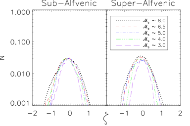
Figure 1.— PDFs of $ln(\Sigma/\Sigma_{0})$. The left panel shows sub-Alfvénic models and the right panel shows super-Alfvénic models. All models plotted here have resolution $512^{3}$. All models show log-normal PDFs over a range of sonic and Alfvénic Mach number.

The density variance- ${\cal M}_{s}$ relationship of Equation 2 has only one fit parameter, and here we have chosen a two-parameter fit with $b$, and $A$. However, due to the similarity between column density and density statistics, we can take the value of $b$ to be the value expected for solenoidal driving, i.e. $b=1/3$. In this case, we find the best fit $A$ to be $A=0.11$. We plot the column density variance- ${\cal M}_{s}$ relationship in Figure 2 for the logarithmic distribution ($\zeta$, top) and the linear distribution (bottom). Blue symbols are for sub-Alfvénic simulations and black for super-Alfvénic cases. Diamond symbols represent simulations with resolution for $256^{3}$ while asterisk symbols are for cases with resolution $512^{3}$. Error bars are created by taking the standard deviation of values between different sight lines. The black dotted line represents Equation 3 and 4 with $A=0.11$ and $b=1/3$ for the top and bottom plots, respectively.

The column density variance- ${\cal M}_{s}$ relationship is narrower for low values of sonic Mach number and slightly wider at higher sonic Mach numbers. This is due to observing at filamentary supersonic turbulence along different sight-lines. Examination of Figure 2 shows that the column density variance- ${\cal M}_{s}$ has a slight dependency on the magnetic field within the error bars, however it is not a overwhelming trend. This was also reported in other studies of PDF moments (Kowal, Lazarian, & Beresnyak 2007). There is a general increase of the variance with sub-Alfvénic turbulence, which can also be visibly seen in Figure 1. This is probably related to the effects studied in Molina et al. (2012), who found that the $\sigma^{2}_{\rho/\rho_{0}}$-${\cal M}_{s}$ relationship has a dependency on the plasma $\beta$ in the super-Alfvénic MHD regime and that this relation breaks down in the sub-Alfvénic regime due to increased anisotropy. In the case of column density, an additional parameter that will affect the observed anisotropy is the line-of-sight chosen. Both the level of the observed anisotropy and the correlations between $\rho$ and B change as the line-of-sight changes (Burkhart et al. 2009). In this case, it is beyond the scope of this letter to examine how the observed line-of-sight changes the $\sigma^{2}_{\rho/\rho_{0}}$-${\cal M}_{s}$ relationship of Molina et al. (2012) when translated to 2D column density.

We find that there is no substantial difference between models with $256^{3}$ and $512^{3}$ resolution at the currently studied sonic Mach numbers. This is not surprising in the context of other works that studied the density variance. Price & Federrath (2010) found that the PDFs for both grid and SPH codes at $256^{3}$ and $512^{3}$ converge. However, PFB11 found that, at-${\cal M}_{s}>5$ the linear variance was affected by numerical resolution, while logarithmic variance is independent of numerical resolution. At ${\cal M}_{s}>5$ our simulations become more spread about the expected trend, however it is not clear if this is due to numerical issues or line-of-sight effects. Future column density studies extending to higher values of ${\cal M}_{s}$ are needed to confirm this.

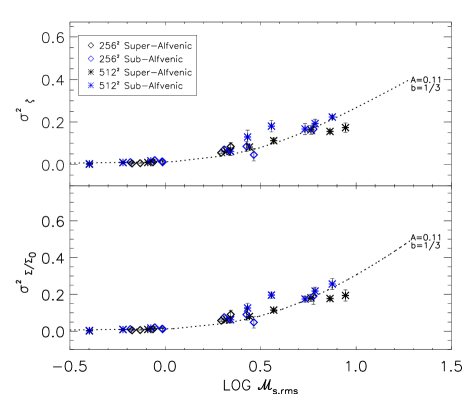
Figure 2.— The column density variance- ${\cal M}_{s}$ relationship ($\sigma_{\Sigma/\Sigma_{0}}^{2}$ vs ${\cal M}_{s}$). Blue symbols are for sub-Alfvénic simulations and black for super-Alfvénic cases. Diamond symbols represent simulations with resolution for $256^{3}$ while astrix symbols are for cases with resolution $512^{3}$. Error bars are created by taking the standard deviation of values between different sight lines. The black dotted lines represent Equation 3 and 4 with $A=0.11$ and $b=1/3$ for the top and bottom plots, respectively.

3.1. Observations

With the wealth of integrated intensity and dust extinction maps, why are there so few observational studies investigating the relationship between $\sigma^{2}$-${\cal M}_{s}$? The answer, in part, is because it is not straightforward to calculate $\sigma^{2}_{\rho/\rho_{0}}$ from $\sigma^{2}_{\Sigma/\Sigma_{0}}$, which is required for the application of Equation 2. Brunt (2010) and PFB11 investigated the relationship of $\sigma_{\rho/\rho_{0}}^{2}$-${\cal M}_{s}$ for Taurus and calculated the column density variance using a combination of ¹³CO and dust extinction maps. They found ${\cal M}_{s}\approx 17.6\pm 1.8$ for Taurus using velocity dispersions. However, this value was calculated incorrectly and an erratum is in preparation. The corrected value of ${\cal M}_{s}$ for Taurus is $\approx 10$ (private communication with C. Brunt, also see Kainulainen & Tan 2012). Brunt (2010) finds $\sigma_{\Sigma/\Sigma_{0},Av}^{2}=0.7\pm 0.04$ (with the error coming from the noise variance) for the Taurus dust extinction maps taken from Froebrich et al. (2007). Although Brunt (2010) used the ¹³CO and the dust extinction maps to obtain the underlying column density variance, we feel that the use of the dust maps is more reliable due to a number of effects (i.e.¹³CO is more susceptible to excitation effects, optical depth effects, and has a small dynamic range of density), which we detail more in Section 4. In addition to the Taurus molecular cloud, Padoan et al. 1997 investigated the $\sigma^{2}$-${\cal M}_{s}$ in the cloud IC 5146 using dust extinction observations by Lada et al. (1994). They found ${\cal M}_{s}\approx 10$ and $\sigma_{\Sigma/\Sigma_{0},Av}^{2}=0.49\pm 0.01$, which they then used to convert to a 3D density variance. The values of $b$ are conservatively constrained from $0.3-0.8$ for these molecular clouds (Brunt 2010) with $b=0.48-0.5$ being the most agreed upon value (Padoan et al. 1997; Brunt 2010). For Taurus, the value of $b$ is still $\approx$ 0.5 despite the change in the sonic Mach number (see Kainulainen & Tan 2012).

Because we are interested in investigating how the $\sigma_{\Sigma/\Sigma_{0}}^{2}$-${\cal M}_{s}$ relationship can be directly applied to the observations, we must consider the effects of instrument noise and telescope smoothing on our synthetic column density maps. We apply Gaussian white noise with mean signal-to-noise=100 and smoothing with a Gaussian beam to the models listed in Table 1. We choose a beam size of 4.6 arcminutes, with an assumed distance to our ’cloud’ of 140pc and a cloud size of 24pc.

We plot the column density variance derived from the dust extinction maps for Taurus and IC 5146 and our models from Table 1, which now include 4.6 arcminute smoothing and Gaussian noise, in Figure 3, in order to test our $\sigma^{2}$-${\cal M}_{s}$ relationship given in Equation 3 and 4 on the observations. The linear column density variance- ${\cal M}_{s}$ relationship is shown in the bottom panel and the logarithmic distribution ($\zeta$) in the top panel. Blue symbols are for sub-Alfvénic simulations and black for super-Alfvénic simulations. Diamond symbols represent simulations with resolution for $256^{3}$ while asterisk symbols are for cases with resolution $512^{3}$. The black lines represent Equation 3 and 4 (for the top and bottom plots, respectively) with $b=1/3$ and $A=0.11$ for the isothermal simulations and $b=0.5$ and $A=0.16$ and $b=0.5$ and $A=0.12$ for Taurus and IC 5146, respectively. The green and red triangles are the $\sigma_{\Sigma/\Sigma_{0}}^{2}$-${\cal M}_{s}$ values from the dust extinction maps for the IC 5146 and Taurus molecular clouds, as given by Padoan et al. (1997) and Brunt (2010), respectively.

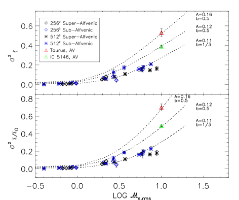
Figure 3.— Similar to Figure 2 only now the synthetic column density maps include smoothing and Gaussian noise. The trend is unaffected at lower Mach number regimes, however at high sonic Mach number (${\cal M}_{s}>7.0$) the values for $\sigma^{2}$ show slightly more of a decrease in variance due to shocks being smoothed over. The Taurus (red triangle; Brunt 2010) and IC 5146 (green triangle; Padoan et al. 1997) clouds are included along with the fits from Equations 3 and 4.

Comparison of Figure 2 (where no smoothing is included) with Figure 3 shows that the inclusion of smoothing and noise, at least at the level added here, does not severely affect the applicability of Equations 3 and 4. In general, smoothing decreases the value of $\sigma^{2}$, causing one to underestimate ${\cal M}_{s}$.

The values for the Taurus and IC 5146 clouds lie very close to what is expected from Equations 3 and 4 for $b=0.5$ and $A=0.16$ and $b=0.5$ and $A=0.12$, respectively. Although Equations 3 and 4 fit well, it is clear that the solenoidal simulations do not fit well with the molecular cloud data. This was also the case in PFB11, who attributed the discrepancy between their simulations and observations to the lack of self-gravity and/or use of purely solenoidal forcing. For PFB11 the assumptions involved to convert the 2D to 3D variance and the use of CO in the variance calculation may also effect the relation. The fact that the dust extinction observations are able to fit Equations 3 and 4 using the values of $b$ obtained from previous studies opens up the prospects of using the 2D column density variance in addition to the assumed 3D variance. Additionally, the parameter $A$ may have dependencies on other physics, which are discussed below.

4. Discussion

In this letter we found a relation between the variance of column density and ${\cal M}_{s}$. The 3D density variance relationship of Equation 2 was modified to obtain the $\sigma^{2}$-${\cal M}_{s}$ relationship for column density. This was motivated by the fact that $\sigma_{\rho/\rho_{0}}^{2}$ is not available from observations. Ideally, both $\sigma_{\rho/\rho_{0}}^{2}$, as determined by the method outlined in Brunt, Federrath, Price (2010), and the direct $\sigma_{\Sigma/\Sigma_{0}}^{2}$-${\cal M}_{s}$ relationship outlined here should be used together to provide more confidence in the $\sigma^{2}$-${\cal M}_{s}$ relation and help constrain the values of $b$.

Furthermore, the results of this letter can be used synergistically with higher order PDF moments suggested in a number of recent papers (see Kowal et al. 2007, Burkhart et al. 2009) to study ${\cal M}_{s}$. The use of different approaches in determining ${\cal M}_{s}$ from observed column densities including other techniques, e.g. utilizing Tsallis statistics (Esquivel & Lazarian 2010, Tofflemire et al. 2011) and the genus measure (see Burkhart, Lazarian & Gaensler 2012), can further increase the reliability of the results obtained.

An additional complicating factor for the observations is that obtaining the true column density PDF can be tricky (Goodman, Pineda & Schnee 2009). In general, the use of dust extinction maps is more reliable than ¹³CO in order to obtain the true column density for a variety of reasons, including a larger dynamic range (factors of 50 or more, see Goodman, Pineda & Schnee 2009, for more detailed discussion). Pineda, Caselli,& Goodman (2008) showed that the ¹³CO derived column density estimates are adversely effected by optical depth as low as A_v $\approx$ 4 mag. Molecular transitions have a limited range of volume densities that they can trace, since below a critical density there may not be enough molecules to excite the transition and at very high densities optical depth effects will mask the true column density. For these reasons, we chose to plot the values of $\sigma^{2}$ for Taurus and IC 5146 taken from the dust extinction maps, rather than the ¹³ CO maps.

Parameters $A$ and $b$ have dependencies on external physics beyond the sonic Mach number. $b$ depends on the driving of the turbulence and it is possible that $A$ may follow the same behavior. In order to test this, we take values from Table 3 of Federrath et al. 2010, with $\sigma_{\Sigma/\Sigma_{0},sol}^{2}$=0.46 and $\sigma_{\Sigma/\Sigma_{0},com}^{2}$=1.51 and ${\cal M}_{s}$=5.5. We note that these values are taken from simulations that have purely solenoidal or purely compressive forcing, when in realty molecular clouds most likely have turbulence driven with mixed forcing. We find that applying these values to Equation 3 yields $A_{sol}=0.14$ and $A_{com}=0.6$. However, when using a simple scaling between $\sigma_{\Sigma/\Sigma_{0}}$ and $\sigma_{\rho/\rho_{0}}$ (given in Table 1 of Federrath et al. 2010), we find that $A_{sol}=0.12$ and $A_{com}=0.25$. Both methods show that the parameter $A$ has a significant dependency on the type of driving, however there is large variation in the compressive driven values of $A$ based on these tables, which may be due to LOS effects or insufficient statistics. Additionally, some dependency on observational effects such as beam smoothing and noise was seen in Figure 3 and future studies will determine what the effects of optical depth my have on these parameters.

The fact of the matter is that the variance of the density or column density distribution does not only depend on the sonic Mach number, but a host of other contributing factors. This is strong motivation for the use of multiple tools and techniques to obtain information on the turbulent state of the gas. A collaborative use of PDF methods that include the 3D and 2D variance as well as higher order moments of the linear distribution will yield the most accurate picture.

5. Conclusions

We investigate the utility of a 2D column density $\sigma_{\Sigma/\Sigma_{0}}^{2}$-${\cal M}_{s}$ trend which can be used in addition to the existing 3D density $\sigma_{\rho/\rho_{0}}^{2}$-${\cal M}_{s}$ trend. We find that:

• Equations 3 and 4 (for logarithmic and linear variance, respectively) empirically fit synthetic column density maps well, even when including observational effects such as smoothing and noise, with $b=1/3$ (as appropriate for the solenoidal forcing used in this study, see Federrath et al. 2008) and $A=0.11$.

• For the dust extinction maps of the Taurus and IC 5146 molecular clouds, we find $A=0.16$ and $A=0.12$, respectively, when using $b=0.5$ (as given in the literature) for the $\sigma_{\Sigma/\Sigma_{0}}^{2}$-${\cal M}_{s}$ relation.

References

- Armstrong et al. (1995) Armstrong,J. W., Rickett, B. J., Spangler, S. R., 1995, ApJ, 443, 209
- Beetz et al. (2008) Beetz, C., Schwarz, C., Dreher, J., & Grauer, R. 2008, Phys. Lett. A, 372, 3037
- Berkhuijsen & Fletcher (2008) Berkhuijsen E., Fletcher, A., 2008, MNRAS, 390, 19
- Brunt (2010) Brunt, C. M., 2010, A&A 513, A67
- Brunt, Federrath, & Price (2010) Brunt, C. M., Federrath, C., & Price, D. J. 2010, MNRAS, 403, 1507
- Burkhart et al. (2009) Burkhart, B., Falceta-Goncalves, D., Kowal, G., Lazarian, A., 2009, ApJ, 693, 250
- Burkhart et al. (2010) Burkhart, B., Stanimirovic, S., Lazarian, A., Grzegorz, K., 2010, ApJ, 708, 1204
- Burkhart et al. (2011) Burkhart, B., Lazarian, A., Gaensler, B., 2012, ApJ, 708, 1204
- Chepurnov & Lazarian (2010) Chepurnov & Lazarian, 2010, ApJ, 710, 853
- Cho et al. (2003) Cho, J. & Lazarian, A. 2003, MNRAS, 345, 325
- Elmegreen & Elmegreen (1983) Elmegreen, B. G., & Elmegreen, D. M. 1983, MNRAS, 203, 31
- Esquivel & Lazarian (2010) Esquivel, A., & Lazarian, A., 2010, ApJ, 710, 125
- Fed. et al. (2008) Federrath, C., Klessen, R. S., & Schmidt, W , 2008b, ApJ, 688, 79
- Fed. et al. (2010) Federrath, et al., 2010, A&A, 512, A81
- Froebrich et al. (2007) Froebrich, D., Murphy, G. C., Smith, M. D., Walsh, J., & del Burgo, C. 2007, MNRAS, 378, 1447
- Goodman et al. (2009) Goodman, A. A., Pineda, J. E., & Schnee, S. L. 2009, ApJ, 692, 91
- Hennebelle (2008) Hennebelle, P., & Chabrier, G. 2008, ApJ, 684, 395
- Hennebelle (2011) Hennebelle, P., & Chabrier, G., 2011, ApJ, 743, 29
- Heyer & Brunt (2004) Heyer, M., Brunt, C., 2004, ApJ, 615, 45
- Hill et al. (2008) Hill et al., 2008, ApJ, 686, 363
- Kainulainen et al. (2011) Kainulainen, J., Beuther, H., Banerjee, R., Federrath, C., Henning, T., 2011, A&A, 530, 64
- Kainulainen & Tan (2012) Kainulainen, J., & Tan J., 2012, A&A, submitted.
- Kowal et al. (2007) Kowal, G., Lazarian, A. & Beresnyak, A., 2007, ApJ, 658, 423
- Krumholz & Mckee (2005) Krumholz & Mckee, 2005, ApJ, 630, 250
- Lada et al. (1994) Lada et al., 1994, ApJ, 429, 694
- Lazarian (2009) Lazarian, A., 2009, SSR, 143, 357
- Lemaster & Stone (2008) Lemaster, M. N., & Stone, J. M. 2008, ApJ, 682, L97
- Molina et al. (2012) Molina et al., 2012, MNRAS, in press.
- Nordlund (1999) Nordlund, A., & Padoan, P. 1999, in Interstellar Turbulence, ed. J. Franco & A. Carraminana (Cambridge: Cambridge Univ. Press), 218
- Padoan & Nordlund (1997) Padoan, P., Nordlund, A., & Jones, B. J. T. 1997, MNRAS, 288, 145
- Padoan & Nordlund (2011) Padoan, P. & Nordlund, A., 2011, ApJ, 730, 40
- Passot & Vazquez (1998) Passot, T. & Vazquez-Semadeni, E. 1998, Phys. Rev. E, 58, 4501
- Pineda et al. (2008) Pineda, J., Caselli, P., Goodman, A., 2008, ApJ, 679, 481
- Price (2010) Price, D., & Federrath, C., 2010, MNRAS 406, 1659
- Price (2011) Price, D., Federrath, C., & Brunt, C., 2011, ApJ, 727 (PFB11)
- Roman-Duval et al. (2010) Roman-Duval et al., 2010, ApJ, 723, 492
- Sanchez et al. (2005) Sanchez et al. 2005, ApJ, 625, 849
- Spitzer (1979) Spitzer, L., Physical Processes in the Interstellar Medium, 1978, New York: John Wiley & Sons.
- Stutzki & Guesten (1990) Stutzki, J., & Guesten, R., 1990, ApJ, 356, 513
- Stutzki et al. (1998) Stutzki, J., Bensch, F., Heithausen, A., Ossenkopf, V., Zielinsky, M., 1998, A&A, 336,697
- Toffelmire et al. (2011) Toffelmire, B., Burkhart, B., Lazarian, A., 2011, ApJ, 736, 60
- Vazquez-Semadeni (1994) Vazquez-Semadeni, E., 1994, ApJ, 423, 681
- Vazquez-Semadeni & Garcia (2001) Vazquez-Semadeni, E., & Garcia, N., 2001, ApJ, 557, 727