UT-12-10

IPMU-12-0092

YITP-12-43

Naive Dimensional Analysis in Holography
Ryoichi Nishio^1,2, Taizan Watari¹, Tsutomu T. Yanagida¹ and Kazuya Yonekura³

¹ Kavli Institute for the Physics and Mathematics of the Universe (IPMU),
University of Tokyo, Chiba 277-8583, Japan
² Department of Physics, University of Tokyo,
Tokyo 113-0033, Japan
³ Yukawa Institute for Theoretical Physics, Kyoto University,
Kyoto 606-8502, Japan

1 Introduction

It is beneficial to theoretically understand parameters in the low-energy effective theory of hadrons which emerges from a strong dynamics of a gauge theory. Models beyond the standard model sometimes contain a strongly coupled sector (e.g. technicolor models, dynamical supersymmetry breaking models, etc.), and the parameters of the low-energy effective theory of hadrons can be observable or at least relevant to phenomenology. Even within the standard model, the chiral Lagrangian is an effective theory of QCD. Although the parameters of the effective theories such as masses and coupling constants should be determined in terms of parameters in the theories at short distance, it is often difficult to calculate them due to strong coupling.

However, there is an ansatz that is known to be reasonable to some extent; it is called naive dimensional analysis (NDA) [1, 2, 3, 4], which roughly guesses magnitude of coupling constants among hadrons. In the NDA ansatz, the effective action of glueballs is given by

$$S=\int d^{4}x\;\frac{N_{c}^{2}}{(4\pi\beta)^{2}}\;{\cal L}(\phi(x),\partial_{\mu},\Lambda_{\text{NDA}}),$$ (1)

where $\Lambda_{\text{NDA}}$ is a parameter with mass dimension one and fields collectively denoted by $\phi(x)$ represent glueballs. All terms in ${\cal L}(\phi(x),\partial_{\mu},\Lambda_{\text{NDA}})$ are assumed to have dimensionless coefficients of order unity (apart from an appropriate power of $\Lambda_{\text{NDA}}$), and consequently, it follows that $\Lambda_{\text{NDA}}$ is the mass scale of hadrons (except for Nambu-Goldstone bosons). The overall factor $N_{c}^{2}$ should be replaced with $N_{c}$ in the case of effective action of mesons [5, 6], so that the $N_{c}$ scaling rule in a large $N_{c}$ gauge theory is satisfied. The essential point of the NDA ansatz is that the overall factor contains $4\pi$ $(\simeq 13)$, which is sizable compared with unity; this overall prefactor may not precisely be $N_{c}^{2}/(4\pi)^{2}$, but the NDA ansatz assumes that the deviation—represented by a yet undertermined factor $1/\beta^{2}$—is of order unity. After rescaling of $\phi(x)$ so that the $\phi(x)$ fields have canonically normalized kinetic terms, the coefficients of the interaction terms become of the forms, for example,

$$(\partial_{\mu}\phi\partial^{\mu}\phi)\left[\frac{\phi}{\Lambda_{\text{NDA}}}\left(\frac{4\pi\beta}{N_{c}}\right)\right]^{I}\times{\cal O}(1),\quad\Lambda_{\text{NDA}}^{2}\phi^{2}\left[\frac{\phi}{\Lambda_{\text{NDA}}}\left(\frac{4\pi\beta}{N_{c}}\right)\right]^{I}\times{\cal O}(1)$$ (2)

for arbitrary integers $I$ ($\geq 1$); any $(I+2)$-point coupling constants will scale in $I$ as $(4\pi\beta/N_{c})^{I}\times{\cal O}(1)$ in unit of $\Lambda_{\text{NDA}}$. There is an experimental support for the NDA ansatz (1, 2); the coupling constant of three-pion-interaction $(\partial\pi)^{2}\pi$ is $f_{\pi}^{-1}$ in the chiral Lagrangian, and it is reasonably close to the prediction of the NDA ansatz, $\frac{1}{\Lambda_{\text{NDA}}}\left(\frac{4\pi}{N_{c}^{1/2}}\right)$, when experimental values, $f_{\pi}\sim 100$ MeV , $\Lambda_{\text{NDA}}\sim m_{\rho}\sim 1$ GeV and $N_{c}=3$ are substituted.

There are a couple of different ways to argue in favor of the NDA ansatz (1) also from theoretical perspectives. One of them is to require an ansatz of “loop saturation” in loop calculation in the effective theory. The loop saturation ansatz requires that each loop contribution to an amplitude is comparable to the tree level one, if the external momenta are taken to be of order $\Lambda_{\text{NDA}}$ and the UV-cutoff of loop momenta is also set to be $\Lambda_{\text{NDA}}$. It follows from this ansatz that $(I+2)$-point coupling constants among arbitrary hadrons are ${\cal O}((4\pi)^{I})$. However, the result seems to be incompatible with the $N_{c}$ scaling law, because the $(I+2)$-point coupling constants of glueballs should be proportional to $N_{c}^{-I}$ in a large $N_{c}$ gauge theory. If one multiplies $(4\pi)^{I}$ by adequate powers of $N_{c}$ in order to satisfy the correct $N_{c}$ scaling law, one obtains the NDA ansatz (1).

Another argument for the ansatz (1, 2) is based on the large $N_{c}$ expansion. Suppose that an operator ${\cal O}$ is a single trace operator such as $\text{Tr}(FF)$ which can create glueball states $|h_{n}\rangle$, $\langle\text{vac}|{\cal}O(x)|h_{n}({\mathbf{p}})\rangle=f_{n}e^{ipx}$. The $(I+2)$-point correlation function is given in planar limit by

$$\langle{\cal O}(p_{1}){\cal O}(p_{2})\dots\cal O(p_{I+2})\rangle=(2\pi)^{4}\delta^{4}(\sum_{i}p_{i})J_{I+2}(\lambda;{p_{i}})\frac{N_{c}^{2}}{16\pi^{2}}.$$ (3)

If the ’t Hooft coupling $\lambda=g_{\text{YM}}^{2}N_{c}$ is small, $J_{I+2}(\lambda;p_{i})$ can be calculated perturbatively in the gauge theory and it is given schematically by

$$J_{I+2}(\lambda;p_{i})\sim p^{d(I+2)+4}\times\left[{\cal O}(1)+{\cal O}\left(\frac{\lambda}{16\pi^{2}}\right)+{\cal O}\left(\frac{\lambda}{16\pi^{2}}\right)^{2}+\dots\right],$$ (4)

where $d$ is the dimension of the operator ${\cal O}(p)$. The last factor $N_{c}^{2}/(16\pi)^{2}$ comes from two color loops of gluons and a loop factor. For large $\lambda$, perturbation breaks down and we do not know the form of $J_{I+2}(\lambda;p_{i})$. If we knew $J_{I+2}(\lambda;p_{i})$ for large $\lambda$, we could read mass spectra $m_{n}$, decay constants $f_{n}$, and coupling constants $g_{n_{1}\dots n_{I+2}}$ of glueballs from the behavior of $J_{I+2}(\lambda;p_{i})$ around mass poles $p_{i}^{2}\rightarrow-m_{n_{i}}^{2}$ of each external momenta;

$$J_{2}(\lambda;p_{i})\frac{N_{c}^{2}}{16\pi^{2}} \sim\frac{f_{n}^{2}}{p_{1}^{2}+m_{n}^{2}}, J_{I+2}(\lambda;p_{i})\frac{N_{c}^{2}}{16\pi^{2}} \sim\prod_{i=1}^{I+2}\left(\frac{f_{n_{i}}}{p_{i}^{2}+m^{2}_{n_{i}}}\right)\times g_{n_{1}\dots n_{I+2}}.$$ (5)

If we assume that the unknown functions $J_{I+2}(\lambda;p_{i})$ are of the form $p^{d(I+2)+4}\times{\cal O}(1)$ as in the case of small ’t Hooft coupling, we may obtain

$$f_{n} \sim m^{d+3}\left(\frac{N_{c}}{4\pi}\right) g_{n_{1}\dots n_{I+2}}\sim m^{-I+2}\times\left(\frac{4\pi}{N_{c}}\right)^{I},$$ (6)

where $m$ is the typical mass scale of glueballs. The second expression is in accordance with the NDA ansatz (1).

Both of the above two arguments, however, are far from being a clear justification for the NDA ansatz. The loop saturation in the first argument is an ansatz in itself. Moreover, the apparent contradiction between the loop saturation and the $N_{c}$ scaling may cast doubt on the reasoning of loop saturation. One may not be satisfied with the second argument either, because the estimation for the Green functions $J_{I+2}(\lambda;p_{i})$ from perturbative calculation has no justification for a large ’t Hooft coupling.

In this article, we study the NDA ansatz (1) by means of gauge/string duality [7, 8, 9] for some types of scalar glueballs. Although the NDA has been checked only by experimental values of $f_{\pi}$ etc. in QCD so far, the gauge/string duality provides us with plenty of strongly coupled gauge theories which are calculable in the gravity duals. We leave a study of the NDA for other types of hadrons (such as glueballs with higher spin and flavor non-singlet mesons) for future work. The rest of the paper is organized as follows. In section 2, the glueball coupling constants are given in terms of the language of a string theory. They include overlap integrals which we cannot calculate analytically. We will verify the NDA by giving a generic estimation for the overlap integrals. In section 3, we confirm the estimation and the NDA scaling rule by numerical calculation in two specific gravity backgrounds. In section 4, we briefly summarize our study.

Mass spectra and several three or four point couplings among composite states have already been studied by means of gauge/string duality in [10, 11, 12, 13, 14, 15, 16] in several gravitational models. Our aim in this article is to find a rule governing the behavior of large numbers of coupling constants, not only three or four point couplings but generally $(I+2)$-point couplings.

Note also that we will not only verify the NDA ansatz (1, 2), which is for $SU(N_{c})$ gauge theories. In this paper, we derive an extended version of NDA scaling rule, which cover more general gauge theories (such as a class of quiver gauge theories where the gauge group contains $p$ copies of $SU(N_{c})$). In the extended version of the NDA scaling rule, $N_{c}$ in the overall factor in (1) will be replaced with $\sqrt{a}$ multiplied by an ${\cal O}(1)$ factor, where $a$ is something like a “degree of freedom” of a gauge theory.

2 Glueball Coupling Constants in Gauge/String Duality

In the gauge/string duality [7, 8, 9], some gauge theories with a large number of color $N_{c}$ and a large ’t Hooft coupling $\lambda=g_{YM}^{2}N_{c}$ are dual to string theories on warped spaces. A gravity dual of a four-dimensional conformal field theory is the type-IIB string theory on a spacetime $AdS_{5}\times W$ with a metric

$$ds^{2}=R^{2}/z^{2}(\eta_{\mu\nu}dx^{\mu}dx^{\nu}+dz^{2})+R^{2}ds_{W}^{2},\quad 0<z<\infty,$$ (7)

where $W$ is a five-dimensional Einstein manifold. An infinite number of examples of $W$ are known, with each manifold $W$ corresponding to a conformal field theory. For example, the Type IIB string with $W=S^{5}$ is dual to ${\cal N}=4$ $SU(N_{c})$ super Yang-Mills theory [7], and a choice $W=T^{1,1}$ corresponds to an ${\cal N}=1$ $SU(N_{c})\times SU(N_{c})$ gauge theory with four chiral multiplets in the bifundamental representation [17]. In references [18, 19], one can find an infinite number of examples of gravity background geometries with $W=Y^{p,q}$, which correspond to $(SU(N_{c}))^{p}=SU(N_{c})\times SU(N_{c})\times\cdots\times SU(N_{c})$ ($p$ factors of $SU(N_{c})$) quiver gauge theories with several chiral multiplets in the bifundamental representations between two of the $p$ $SU(N_{c})$ groups.

Gravity duals of confining gauge theories have also been constructed [20, 21, 22, 23, 24]. In most of them, the metric background in the string frame may be written without loss of generality as,

$$ds^{2}=(f(z))^{-2}(\eta_{\mu\nu}dx^{\mu}dx^{\nu}+dz^{2})+R^{2}ds_{W_{z}}^{2},$$ (8)

with an appropriate definition of the $z$-coordinate. The warp factor $R^{2}/z^{2}$ in (7) for the case of conformal theories is replaced by a more general form $(f(z))^{-2}$. The internal manifold $W_{z}$ can also be dependent on $z$, and the other supergravity fields generally have nontrivial background. Although details of the background are model dependent, most of the gravitational models which are dual to confining gauge theories have at least one thing in common; the radial coordinate terminates at finite value $z=z_{\text{max}}$. Normalizable wavefunctions of the fluctuations of supergravity fields around their backgrounds become discrete like cavity modes when the range of the radial coordinate ($0<z<z_{\text{max}}$) is finite. Each composite state, i.e. glueball, in a gauge theory is described by each normalizable wavefunction in the dual gravity theory. The quantity $z_{\text{max}}$ corresponds to the mass scale of glueballs in the gauge theory.

The four dimensional effective action of glueballs is obtained by dimensional reduction: expanding the fields in the ten dimensional type-IIB supergravity action in terms of the complete set of wavefunctions on the radial and compact directions and integrating over those directions. We can carry out this procedure by two steps of dimensional reduction; the first step is to construct a five dimensional supergravity action by integrating the complete set on the five dimensional compact manifold $W_{z}$, and the second step is to obtain the four dimensional effective action of glueballs by integrating the complete set on the radial $z$-coordinate.

2.1 An Intermediate Description in Five Dimensions

In order to examine how glueball couplings are controlled in gauge/string duality, we start from dimensional reduction on five dimensional internal manifold in the case of the conformal background (7). It is useful to study the conformal case first, before going to the confining case (8), because the conformal background (7) approximates the confining background (8) to some extent, except for deep IR-region $z\sim z_{\text{max}}$.

In the case of the conformal background $AdS_{5}\times W$ (7), dilaton has constant background, $e^{\langle\Phi\rangle}=g_{s}$, and the self dual five form $F_{5}=(1+*){\cal F}_{5}$ has background ${\cal F}_{5}=\frac{(2\pi\sqrt{\alpha^{\prime}})^{4}}{\text{Vol}(W)}N_{c}\;\text{vol}(W)$, where $\text{vol}(W)$ is the volume form of $W$ and $\text{Vol}(W)$ is its volume; $\text{Vol}(W)=\int_{W}\text{vol}(W)$. The backgrounds of the other fields, $C_{0}$, $B_{2}$ and $C_{2}$, are constant, which we assume to be zero for simplicity. After dimensional reduction on the five dimensional compact manifold $W$, the supergravity action using the Einstein frame metric becomes

$$S=\frac{(R^{5}\text{Vol}(W))\times R^{3}}{2\kappa_{10}^{2}g_{s}^{2}}\int d^{4}x\int^{\infty}_{0}\frac{dz}{z^{3}}\left(-\frac{1}{2}((\partial\phi)^{2}+(\partial_{z}\phi)^{2})-\frac{1}{2}e^{2\phi}((\partial c)^{2}+(\partial_{z}c)^{2})\right)+\dots,$$ (9)

where ${2\kappa_{10}^{2}}=(2\pi)^{7}\alpha^{\prime 4}$ is the gravitational coupling constant of ten dimensional type IIB supergravity. Here we only keep track of $\phi(x,z)$ and $c(x,z)$ fields in five dimensions, which correspond to fluctuations of $\Phi$ (dilaton) and $C_{0}$ (RR scalar) with a constant profile on $W$, respectively. The AdS radius $R$ is given by

$$R^{4}=4\pi^{4}g_{s}\alpha^{\prime 2}\frac{1}{\text{Vol}(W)}=4\pi g_{s}\alpha^{\prime 2}\frac{\text{Vol}(S^{5})}{\text{Vol}(W)}.$$ (10)

Then the overall factor is rewritten as

$$\frac{1}{2\kappa_{10}^{2}g_{s}^{2}}\times(R^{5}\text{Vol}(W))\times R^{3}=\frac{4a}{8\pi^{2}},$$ (11)

with the definitions

$$4a\equiv p^{\prime}N_{c}^{2},\quad p^{\prime}\equiv\frac{\text{Vol}(S^{5})}{\text{Vol}(W)}.$$ (12)

The supergravity action (9) becomes an expression that is interesting in the context of the NDA, by canonically rescaling the fields,

$$S=\int d^{4}x\int^{\infty}_{0}\frac{dz}{z^{3}}\left[-\frac{1}{2}((\partial\phi^{\prime})^{2}+(\partial_{z}\phi^{\prime})^{2})-\frac{1}{2}((\partial c^{\prime})^{2}+(\partial_{z}c^{\prime})^{2})\right.$$

$$\left.-\sum_{I=1}^{\infty}\left(\frac{4\pi}{\sqrt{2a}}\right)^{I}\frac{1}{I!2!}(\phi^{\prime})^{I}((\partial c^{\prime})^{2}+(\partial_{z}c^{\prime})^{2})\right].$$ (13)

Here, $\phi^{\prime}=\phi-\langle\Phi\rangle$ and $c^{\prime}=g_{s}c$. The second line plays a role of interaction terms, which comes from the exponential dilaton factor $e^{2\phi}$. Besides combinatoric factors, the $(I+2)$-point interaction terms of the five dimensional fields $\phi^{\prime}$ and $c^{\prime}$ have coefficients $((4\pi)/\sqrt{2a})^{I}$. Although these coefficients are not glueballs coupling constant themselves, this expression (13) is already quite indicative that the coupling constants of glueballs may show the behavior predicted by NDA (1).

We saw that the parameter $a$ in (12) controls the interactions of the closed string fields. The parameter $a$ corresponds to the central charge $a$ of the conformal field theory which is dual to $AdS_{5}\times W$ [27, 28]. The central charge $a$ represents something like degrees of freedom of the conformal field theory. For example, the property $a\propto N_{c}^{2}$ can be understood because degrees of freedom of gluons and other fields in the adjoint representation of $SU(N_{c})$ gauge group are ${\cal O}(N_{c}^{2})$. Moreover, in the gravity dual of $(SU(N_{c}))^{p}$ quiver gauge theory, $p^{\prime}$ defined in (12) is ${\cal O}(p)$ [18, 19], so we have $a\sim pN_{c}^{2}$. This is also reasonable for the interpretation that $a$ is roughly degrees of freedom of the conformal field theory because degrees of freedom of gauge theory with the gauge group $SU(N)^{p}$ should be about $pN_{c}^{2}$. We also find that $a$ has a lower bound $4a\geq N_{c}^{2}$ [29] because it is proven that $p^{\prime}$ has a lower bound $p^{\prime}\geq 1$ in general Einstein manifold. Therefore, the parameter $a$ makes the couplings in (13) always smaller than $(4\pi)^{I}$.

2.2 Effective Action in Four Dimensions

In order to obtain the effective action of glueballs on the four dimensional spacetime, we also have to integrate the fifth coordinate $z$. The supergravity action on $AdS_{5}$ (9, 13) is no longer suitable for this purpose, because conformal theories do not give rise to a discrete hadron spectrum. We start to consider supergravity on confining geometries (8) instead, and describe coupling constants of glueballs.

Let us first consider a theory which is asymptotically conformal in the UV region. In this case, only minor modification to the five-dimensional description (9, 13) is necessary. In the gravity dual language, $(f(z))^{-2}\simeq(R/z)^{2}$ in the $z\rightarrow 0$ limit, and the central charge $a$ in the UV limit is defined by (12) by using $\text{Vol}(W_{z})$ at $z=0$. On such a geometry, with the same rescaling of the fields as in (13), the five dimensional supergravity action is written as

$$S=\int d^{4}x\int^{z_{\text{max}}}_{0}\frac{dz}{z^{3}}Y(z)\left[-\frac{1}{2}((\partial\phi^{\prime})^{2}+(\partial_{z}\phi^{\prime})^{2})-\frac{1}{2}((\partial c^{\prime})^{2}+(\partial_{z}c^{\prime})^{2})\right.$$

$$\left.-\frac{1}{2!I!}\sum_{I=1}^{\infty}\left(\frac{4\pi}{\sqrt{2a}}\right)^{I}(\phi^{\prime})^{I}((\partial c^{\prime})^{2}+(\partial_{z}c^{\prime})^{2})\right]+\dots,$$ (14)

where $Y(z)$ is a dimensionless function defined as

$$Y(z)=\frac{(f(z))^{-3}}{(R/z)^{3}}\frac{\text{Vol}(W_{z})}{\text{Vol}{(W_{z=0})}},$$ (15)

which is unity in the case of conformal geometries. In the $z\rightarrow 0$ (UV) limit, $Y(z)\rightarrow 1$, and the integrand of (14) becomes identical to one of (13).

In the rest of this article, we omit the terms in $+\cdots$ in (14). In general confining geometry, dilaton, RR scalar and the 3-form flux $H_{3}$ and $F_{3}$ would also have nontrivial background. In this case $\phi^{\prime}(x,z)$ and $c^{\prime}(x,z)$ would have mixings with other string fields such as the metric. We neglect this technical complexity in this article. We expect that such details of the IR background will affect coupling constants of glueballs at most by ${\cal O}(1)$ factors, and hence they are unessential in trying to verify the NDA ansatz, whose predictions always come with uncertainty of order unity.

We denote four dimensional glueball fields of the $n$-th excited modes by $\tilde{\phi}_{n}(x)$ and $\tilde{c}_{n}(x)$, which are created by operators dual to five-dimensional supergravity fields $\phi^{\prime}(x,z)$ and $c^{\prime}(x,z)$, respectively. We assign mass dimension one for glueball fields $\tilde{\phi}_{n}(x)$ and $\tilde{c}_{n}(x)$ just as usual for canonically normalized scalar fields in four dimensional field theory. The five dimensional fields $\phi^{\prime}(x,z)$ and $c^{\prime}(x,z)$ are decomposed into independent modes in four-dimensions, each one of which corresponds to a normalizable wavefunction $\psi_{n}(z)$;

$$\phi^{\prime}(x,z)=\sum_{m=1}^{\infty}\psi_{m}(z)\tilde{\phi}_{m}(x),\quad c^{\prime}(x,z)=\sum_{n=1}^{\infty}\psi_{n}(z)\tilde{c}_{n}(x).$$ (16)

The normalizable modes $\psi_{n}(z)$ are defined as the solutions of the eigen-equation given by

$$z^{3}Y^{-1}(z)\partial_{z}\left(z^{-3}Y(z)\partial_{z}\psi_{n}(z)\right)=m_{n}^{2}\psi_{n}(z),$$ (17)

with the normalization condition

$$\int_{0}^{z_{\text{max}}}\frac{dz}{z^{3}}Y(z)\psi_{n}(z)\psi_{m}(z)=\delta_{nm},$$ (18)

which makes all the fields $\tilde{\phi}_{n}(x)$ and $\tilde{c}_{n}(x)$ canonically normalized in the 4D effective action. The modes $\psi_{n}(z)$ satisfies an appropriate IR-boundary condition which is imposed so that the field configuration in ten dimensional spacetime should be smooth at $z=z_{\text{max}}$. The eigenvalue $m_{n}$ is the mass of glueballs $\tilde{\phi}_{n}$, $\tilde{c}_{n}$. The effective action of glueballs is obtained by substituting (16) to (14).

The interaction part of the effective Lagrangian ${\cal L}_{\text{int}}$ includes $(I+2)$-point interaction terms which consist of two types of couplings; one is of the form $\tilde{\phi}_{m}^{I}(\partial\tilde{c}_{n})^{2}$, and the other $\tilde{\phi}_{m}^{I}\tilde{c}_{n}^{2}$ without derivatives:

$${\cal L}_{\text{int}}=-\sum_{I=1}^{\infty}\sum_{n_{1}n_{2}m_{1}\dots m_{I}} \left[a^{(I)}_{n_{1}n_{2},m_{1}\dots m_{I}}\frac{\Lambda^{-I}_{\text{NDA}}}{2!I!}\tilde{\phi}_{m_{1}}\dots\tilde{\phi}_{m_{I}}(\partial_{\mu}\tilde{c}_{n_{1}})(\partial^{\mu}\tilde{c}_{n_{2}})\right.$$

$$\left.+b^{(I)}_{n_{1}n_{2},m_{1}\dots m_{I}}\frac{\Lambda^{2-I}_{\text{NDA}}}{2!I!}\tilde{\phi}_{m_{1}}\dots\tilde{\phi}_{m_{I}}\tilde{c}_{n_{1}}\tilde{c}_{n_{2}}\right].$$ (19)

The coupling constants $a^{(I)}_{n_{1}n_{2}m_{1}\dots m_{I}}$ and $b^{(I)}_{n_{1}n_{2}\dots m_{1}\dots m_{I}}$ are given by the following overlap integral of normalizable wavefunctions;

$$a^{(I)}_{n_{1}n_{2}m_{1}\dots m_{I}} =\left(\frac{4\pi}{\sqrt{2a}}\right)^{I}\times\Lambda^{I}_{\text{NDA}}\int_{0}^{z_{\text{max}}}\frac{dz}{z^{3}}Y(z)\psi_{n_{1}}\psi_{n_{2}}\psi_{m_{1}}\dots\psi_{m_{I}},$$ (20)

$$b^{(I)}_{n_{1}n_{2}m_{1}\dots m_{I}} =\left(\frac{4\pi}{\sqrt{2a}}\right)^{I}\times\Lambda^{I-2}_{\text{NDA}}\int_{0}^{z_{\text{max}}}\frac{dz}{z^{3}}Y(z)(\partial_{z}\psi_{n_{1}})(\partial_{z}\psi_{n_{2}})\psi_{m_{1}}\dots\psi_{m_{I}}.$$ (21)

These coupling constants have been made dimensionless by multiplying appropriate powers of a parameter $\Lambda_{\text{NDA}}$ with mass dimension one. When we choose the mass scale $\Lambda_{\text{NDA}}$ as the mass of the lightest glueball mass, these coupling constants are expected to be ${\cal O}(4\pi\beta/N_{c})$ by the NDA ansatz (2).

We need to estimate the overlap integrals of (20, 21) in order to examine whether there exists a rule governing the coupling constants of four dimensional effective theory like the NDA ansatz or not. The prefactor $(4\pi/\sqrt{2a})^{I}$ is identical to the coefficient of $(I+2)$-point interaction terms of (13), and is just determined only from conformal region in UV, whereas the remaining overlap integrals are dependent on the detail of the IR geometry. The estimation of the overlap integrals unavoidably requires numerical calculations in each geometry and they will be the subject of section 3. Before numerical calculation, however, we will give a crude estimation independently of the detail of geometries.

We may roughly estimate the overlap integrals for low excited modes and not too large $I$ by approximating the integrand as a constant value in the IR region. On general UV-conformal geometry, normalizable wavefunctions behaves as $z^{\Delta}$ ($\Delta$ is the conformal dimension and $\Delta=4$ for $\phi(x,z)$ and $c(x,z)$) in the small $z$ region, so the small $z$ region have only small contribution to the overlap integrals. They oscillate with relatively large amplitudes in the IR region $z\sim{\cal O}(z_{\text{max}})$, say, $z\gtrsim z_{\text{max}}/2$. The normalizable wavefunctions of the first few excited modes have only a small number of nodes. Then it might be justified to approximate the integrand by a typical constant value in the IR region. Using the value of the integrand at around $z\sim\gamma z_{\text{max}}~{}(\gamma\sim{\cal O}(1))$ as the typical value, the overlap integrals are estimated as

$$|a^{(I)}_{n_{1}n_{2}m_{1}\dots m_{I}}| \sim\left(\frac{4\pi}{\sqrt{2a}}\right)^{I}\Lambda^{I}_{\text{NDA}}z_{\text{max}}^{-2}\left[Y(z)\psi_{n_{1}}\psi_{n_{2}}\psi_{m_{1}}\dots\psi_{m_{I}}\right]_{z\sim\gamma z_{\text{max}}},$$ (22)

$$|b^{(I)}_{n_{1}n_{2}m_{1}\dots m_{I}}| \sim\left(\frac{4\pi}{\sqrt{2a}}\right)^{I}\Lambda^{I-2}_{\text{NDA}}z_{\text{max}}^{-2}\left[Y(z)(\partial_{z}\psi_{n_{1}})(\partial_{z}\psi_{n_{2}})\psi_{m_{1}}\dots\psi_{m_{I}}\right]_{z\sim\gamma z_{\text{max}}}.$$ (23)

Applying the same approximation for bilinear terms, we also obtain

$$\psi_{n}(z\sim\gamma z_{\text{max}})\sim\left[z_{\text{max}}^{-2}Y(z\sim\gamma z_{\text{max}})\right]^{-1/2},\quad\partial_{z}\psi_{n}(z\sim\gamma z_{\text{max}})\sim m\psi_{n}(z\sim\gamma z_{\text{max}}).$$ (24)

We are assuming that $n_{i},m_{j}$ and $I$ are not large, because the integrand would oscillate rapidly if they were large and the above estimation would break down. Here, $\gamma z_{\text{max}}$ is a typical value of $z$ around which the integrand is peaked, and should be near the IR boundary, say, $\gamma\sim 1/2$, and $m$ is a typical mass of the low excited modes (say, $m=m_{1}$). Substituting (24) to (22, 23), we obtain

$$|a^{(I)}_{n_{1}n_{2}m_{1}\dots m_{I}}| \sim\left[\left(\frac{4\pi}{\sqrt{2a}}\right)\Lambda_{\text{NDA}}z_{\text{max}}\left(Y(z\sim\gamma z_{\text{max}})\right)^{-1/2}\right]^{I},$$ (25)

$$|b^{(I)}_{n_{1}n_{2}m_{1}\dots m_{I}}| \sim\left(\frac{m}{\Lambda_{\text{NDA}}}\right)^{2}\left[\left(\frac{4\pi}{\sqrt{2a}}\right)\Lambda_{\text{NDA}}z_{\text{max}}\left(Y(z\sim\gamma z_{\text{max}})\right)^{-1/2}\right]^{I}.$$ (26)

The reason $b^{(I)}$ has the factor of $(m/\Lambda_{\text{NDA}})^{2}$ is that (23) contains two $(\partial_{z}\psi_{n})$’s.

With these crude approximations, one can find that there is a scaling rule for coupling constants like the NDA ansatz (1). When we choose $\Lambda_{\text{NDA}}$ as the typical mass of glueballs,

$$\Lambda_{\text{NDA}} =m,$$ (27)

both of the $(I+2)$-point coupling constants are estimated as $I$-th powers of the same factor,

$$|a^{(I)}_{n_{1}n_{2}m_{1}\dots m_{I}}|,|b^{(I)}_{n_{1}n_{2}m_{1}\dots m_{I}}| \sim\left[\left(\frac{4\pi}{\sqrt{2a}}\right)mz_{\text{max}}(Y(z\sim\gamma z_{\text{max}}))^{-1/2}\right]^{I}$$

$$\sim\left[\left(\frac{4\pi}{\sqrt{2a}}\right)(mz_{\text{max}})\right]^{I},$$ (28)

where we have also used an approximation $Y(z\sim\gamma z_{\text{max}})\sim 1$ in the second line. The factor $(mz_{\text{max}})$ is expected to be ${\cal O}(1)$ because $1/z_{\text{max}}$ corresponds to confinement scale of dual gauge theory, but this factor turns out to be slightly large in numerical calculations as we will see in the next section. Eq. (28) with the choice of (27) is just the same as what the NDA predicts (1), with the identification of the NDA scaling factor

$$\frac{4\pi\beta}{N_{c}} \sim\left[\left(\frac{4\pi}{\sqrt{2a}}\right)(mz_{\text{max}})\right].$$ (29)

The NDA scaling rule shown in (29) has been generalized from the original NDA (1); the factor $N_{c}/\beta$ in the original NDA rule (1) is generalized into $\sqrt{2a}/(mz_{\text{max}})$. The identification is natural in an $SU(N_{c})$ gauge theory because the factor $\sqrt{2a}/(mz_{\text{max}})$ is actually ${\cal O}(N_{c})$, which corresponds to the assumption of the original NDA that $\beta$ is ${\cal O}(1)$. However, Eq.(29) implies that $\beta$ can take an arbitrarily small value, because $4a/N_{c}^{2}=p^{\prime}$ can be arbitrarily large, for example, in a quiver gauge theory $(SU(N_{c}))^{p}$ with arbitrarily large $p$. On the other hand, we also find that $\beta$ has an upper bound of ${\cal O}(1)$ value because $p^{\prime}$ is bounded as $p^{\prime}\geq 1$.

So far, we have only focused on UV-conformal theories, but it is possible to extend the derivation above in order to cover theories with weakly running couplings even in the UV-limit. To do this, note that the $z$-dependent function $a(z)$ can be defined in gravity side even in non-conformal theories [30]:

$$a(z)=\frac{2\pi^{2}R^{5}}{(2\pi)^{7}g_{s}^{2}\alpha^{\prime 4}}\left(\frac{d}{dz}(f(z)(\text{Vol}(W_{z}))^{-1/3})\right)^{-3}.$$ (30)

One can see that $a(z)$ approaches the value $a$ defined in (12) when the geometry approaches $AdS_{5}\times W$. In a theory which has a weakly running coupling in UV, the function $a(z)$ varies only slowly in $z$, although it may vary rapidly in the deep IR region $z\sim z_{\text{max}}$. Then the above NDA scaling rule (29) is expected to be valid also in such theories by replacing $a$ with $\bar{a}$, a typical value of $a(z)$;

$$\frac{4\pi\beta}{N_{c}} \sim\left[\left(\frac{4\pi}{\sqrt{2\bar{a}}}\right)(mz_{\text{max}})\right].$$ (31)

Here, $\bar{a}=a(z\sim\gamma z_{\text{max}})$, and $z\sim\gamma z_{\text{max}}$ is a typical value of $z$ around which the overlap integral is dominated. The typical value $\bar{a}$ has an ambiguity which is at most ${\cal O}(1)$ factor depending on the choice of $\gamma$ because $a(z)$ is slowly varying, and such uncertainty is already expected in the estimation of this section.

3 Numerical Check

In the previous section, we have verified the NDA scaling rule by a crude estimation of the overlap integrals. However, it is difficult to estimate the error within that crude estimation. If the error in the estimation of (29) were greater than the factor of order $4\pi$, that error would be too large to claim that the NDA really holds. In this section we want to confirm the NDA scaling rule (29, 31) by calculating coupling constants numerically, and checking that they are approximately given by the expected value (28) within the range of ${\cal O}(1)$ factors. We will perform numerical calculations in two specific gravity models. Our results are in considerably good agreement with (29, 31).

3.1 Hard Wall Model

First, we estimate the glueball couplings in “hard wall” model [32], which is regarded as the simplest toy model of IR-confining and UV-conformal gauge theories. The hard wall model simply introduces IR-boundary $z=z_{\text{max}}$ to the geometry (7) which is dual to a conformal field theory. Thus, the 5D action of this model is given by (14) with $Y(z)=1.$ In this article, we choose Dirichlet boundary condition at the IR boundary on the wavefunctions, i.e., $\psi_{n}(z_{\text{max}})=0$ (just for simplicity).

In the hard wall model, the mass spectra and normalizable wavefunctions are well-known. The wavefunction $\psi_{n}(z)$ and mass eigenvalue $m_{n}$ of the $n$-th excited state are

$$\psi_{n}(z) =\frac{\sqrt{2}z^{2}}{z_{\text{max}}}\frac{J_{2}(zm_{n})}{J^{\prime}_{2}(j_{2,n})},\quad m_{n}=j_{2,n}/z_{\text{max}},$$ (32)

where $J_{2}(x)$ is the Bessel function of the second order, and $j_{2,n}$ the $n$-th zero of $J_{2}(x)$; $j_{2,1}\simeq 5.1$, $j_{2,2}\simeq 8.4$, $j_{2,3}\simeq 11$. The dimensionless coefficients of the $(I+2)$-point couplings, $a^{(I)}_{n_{1}n_{2}m_{1}\dots m_{I}}$ and $b^{(I)}_{n_{1}n_{2}m_{1}\dots m_{I}}$, can be calculated by using these wavefunctions in (20, 21).

We calculated these coefficients numerically, and obtained geometric means $a^{(I)}_{\text{typ}}$ and $b^{(I)}_{\text{typ}}$ of the ensemble of the $(I+2)$-point coupling constants involving lower excited states. The result shows that the one of the typical values of the $(I+2)$-point coupling constants, $a^{(I)}_{\text{typ}}$, remains almost an $I$-independent constant of order unity ($c\simeq 0.3\mbox{--}0.4$), after an appropriate scaling behavior is factored out:

$$a^{(I)}_{\text{typ}}\simeq c\times\left(\frac{4\pi}{\sqrt{2a}}(\Lambda_{\rm NDA}z_{\rm max})\times 0.8\right)^{I}.$$ (33)

See Table 1. A similar result was also obtained for the other typical value $b^{(I)}_{\text{typ}}$ of the $(I+2)$-point coupling constants when we take $\Lambda_{\text{NDA}}=m_{1}\simeq 5.1/z_{\text{max}}$.

This numerical result shows that the crude estimates in the previous section are quite accurate on average, and there is no question about the scaling behavior of the $(I+2)$-point coupling constants now. It is worthwhile to note, further, that the scaling factor in (29) in the scaling rule we established is somewhat larger—by a factor of $m_{1}z_{\max}\simeq 5.1$ or so in the hard wall model—than what was expected in the naive dimensional analysis.

Although we have seen so far that the geometric means of $(I+2)$-point coupling constants of hadrons, $a^{(I)}_{\rm typ}$ and $b^{(I)}_{\rm typ}$, follow the scaling rule, such a rule will be of little value if the individual coupling constants $a^{(I)}_{n_{1}n_{2}m_{1}\dots m_{I}}$ and $b^{(I)}_{n_{1}n_{2}m_{1}\dots m_{I}}$ take values wildly different from their averages. Our numerical study shows that the typical range of $|a^{(I)}_{n_{1}n_{2}m_{1}\dots m_{I}}|$ is from $a^{(I)}_{\rm typ}\times[e^{-\sigma^{(I)}_{\ln a}}]$ to $a^{(I)}_{\rm typ}\times[e^{+\sigma^{(I)}_{\ln a}}]$, with $[e^{\sigma^{(I)}_{\ln a}}]\simeq 2.$ in the hard wall model. Similarly, it turns out that $[e^{\sigma^{(I)}_{\ln b}}]\simeq 3$. Thus, the coupling constants are typically within the factor of $2\sim 3$ from their geometric means. With the scaling factor $(4\pi)\times(\Lambda_{\rm NDA}z_{\rm max})$ being much larger than the typical difference among the individual couplings $[e^{\sigma^{(I)}_{\ln}}]$, we see that the scaling rule of the averaged value (33) contains valuable information (albeit statistical) on individual $(I+2)$-point coupling constants.

Table 1: Geometric means $a^{(I)}_{\text{typ}}$ and $b^{(I)}_{\text{typ}}$ and the standard deviations $\sigma^{(I)}_{\ln a}$ and $\sigma^{(I)}_{\ln b}$ calculated numerically in the hard wall model. The standard deviation of $\ln|a^{(I)}_{n_{1}n_{2}m_{1}\dots m_{I}}|$’s, that is, $\sigma^{(I)}_{\ln a}$, is presented in the 3rd column in the form of $\ln[\;\exp(\sigma^{(I)}_{\ln a})\;]$, so that the range of typical values of $|a^{(I)}_{n_{1}n_{2}m_{1}\dots m_{I}}|$ can be easily read out.

	$\displaystyle{a^{(I)}_{\text{typ}}\left(\frac{4\pi}{\sqrt{2a}}\Lambda_{\text{NDA}}z_{\text{max}}\cdot 0.8\right)^{-I}}$	$\sigma^{(I)}_{\ln a}$	$\displaystyle{b^{(I)}_{\text{typ}}\left(\frac{4\pi}{\sqrt{2a}}\Lambda_{\text{NDA}}z_{\text{max}}\cdot 0.8\right)^{-I}}$	$\sigma^{(I)}_{\ln b}$
$I=1$	0.3	$\ln[2.]$	$\left(\frac{m_{1}}{\Lambda_{\text{NDA}}}\right)^{2}\times 0.4$	$\ln[3.]$
$I=2$	0.3	$\ln[2.]$	$\left(\frac{m_{1}}{\Lambda_{\text{NDA}}}\right)^{2}\times 0.3$	$\ln[3.]$
$I=3$	0.4	$\ln[2.]$	$\left(\frac{m_{1}}{\Lambda_{\text{NDA}}}\right)^{2}\times 0.2$	$\ln[3.]$
$I=4$	0.4	$\ln[2.]$	$\left(\frac{m_{1}}{\Lambda_{\text{NDA}}}\right)^{2}\times 0.4$	$\ln[4.]$

3.2 Klebanov-Strassler Metric

One of the flaws of the hard wall model is that the IR-region of the geometry is very ad hoc; the IR-boundary $z_{\text{max}}$ is introduced by hand. Such a crude treatment is meant only to be a simplest toy model imaginable that implements the two essential ingredients of IR confining models: i) finite range of the holographic radius, ${}^{\exists}z_{\rm max}\geq z\geq 0$, and ii) existence of the minimal value of the warped factor $f^{-2}(z)$. It is not meant at all to be a faithful (and hence stable) solution of the equation of motion of the Type IIB string theory.

In a full solution of equations of motion of supergravity, however, the IR boundary $z=z_{\rm max}$ is not a singularity of the background geometry; the spacetime geometry is smooth in ten dimensions, and the internal geometry $W_{z}$ smoothly shrinks at $z=z_{\text{max}}$, and we encounter a “boundary” of the geometry only after the description on 10 dimensions is reduced to that on the five dimensions.

In the following, we construct a toy model using the Klebanov-Strassler metric so that the model captures the above nature of faithful solutions to the equation of motions. With this toy model, where the IR geometry is treated in a more appropriate way than in the hard wall model, numerical calculation is carried out once again, in order to check the validity of the crude estimation of the overlap integration in section 2, and also to see how much individual $(I+2)$-point coupling constants are different from their average. Because the Klebanov-Strassler metric does not asymptote to a pure $AdS_{5}\times W$ metric for some 5-dimensional manifold $W$ in the UV region ($z\sim 0$), but maintains logarithmic running, our toy model using the Klebanov-Strassler metric also serves as an ideal test case of how to deal with the running $a(z)$ function in the NDA scaling rule.

The Klebanov-Strassler background is dual to an ${\cal N}=1$ $SU(N)\times SU(N+M)$ quiver gauge theory with chiral multiplets in the bifundamental representations [22]. This gauge theory experiences a cascade of Seiberg duality, $SU(N)\times SU(N+M)\rightarrow SU(N-M)\times SU(N)$. In the IR, the duality cascade ends when the gauge group becomes $SU(M)$ and confinement occurs. In the UV, the cascade of Seiberg duality continues unlimitedly, and it has weakly running RG flow in the UV; this theory is not UV conformal.

Let us briefly review the Klebanov-Strassler metric, focusing only on the aspects that we need in the following. The background metric is given by [22],

$$ds_{10}^{2} =h^{-1/2}(\tau)dx^{2}+h^{1/2}(\tau)ds_{6}^{2},$$ (34)

$$ds_{6}^{2} =\frac{\epsilon^{4/3}}{2}K(\tau)\left[\frac{1}{3K^{3}(\tau)}[(d\tau)^{2}+(g^{5})^{2}]+\cosh^{2}\left(\frac{\tau}{2}\right)[(g^{3})^{2}+(g^{4})^{2}]\right.$$

$$\qquad\qquad\qquad\qquad\qquad\qquad\qquad\quad\quad\left.+\sinh^{2}\left(\frac{\tau}{2}\right)[(g^{1})^{2}+(g^{2})^{2}]\right],$$ (35)

where $\tau\;(\geq 0)$ is the radial coordinate, $g^{1},\dots,g^{5}$ are basis of 1-forms on the compact five dimensional space, and $\epsilon^{2/3}$ is a parameter with mass dimension $-1$. The two functions appearing in (34, 35) are given by

$$K(\tau)=\frac{(\sinh(2\tau)-2\tau)^{1/3}}{2^{1/3}\sinh(\tau)},\quad h(\tau)=\alpha\frac{2^{2/3}}{4}\int_{\tau}^{\infty}dx\frac{x\coth x-1}{\sinh^{2}x}(\sinh(2x)-2x)^{1/3},$$ (36)

where $\alpha=4(g_{s}M\alpha^{\prime})^{2}\epsilon^{-8/3}$ is a dimensionless constant determined by the dilaton vev, RR 3-form flux $M$ and the parameter $\epsilon^{2/3}$. We can rewrite the metric (34) into the form (8), by defining the holographic coordinate $z$ and the function $f(z)$ in (8) as

$$\frac{dz}{d\tau}=-\frac{\epsilon^{2/3}}{\sqrt{6}}\frac{(h(\tau))^{1/2}}{K(\tau)},\quad z(\tau=\infty)=0,\quad f^{2}(z)=(h(\tau))^{1/2}.$$ (37)

In the UV limit ($\tau\rightarrow\infty$, $z\rightarrow 0$), the asymptotic form of $K(\tau)$ and $h(\tau)$ are given by $K(\tau)\rightarrow 2^{1/3}e^{-\tau/3}$ and $h(\tau)\rightarrow\alpha 2^{-5/3}3\tau e^{-4\tau/3}$, respectively, and hence the new holographic coordinate $z$ is related to the original one $\tau$ by $z\rightarrow\alpha^{1/2}\epsilon^{2/3}2^{-5/3}3\tau^{1/2}e^{-\tau/3}$ asymptotically. The asymptotic form of the metric [33] is given (in this coordinate $z$) by,

$$ds_{10}^{2}\rightarrow\frac{R^{2}}{z^{2}}(\ln(z_{0}/z))^{1/2}(\eta_{\mu\nu}dx^{\mu}dx^{\nu}+dz^{2})+R^{2}(\ln(z_{0}/z))^{1/2}ds_{T^{1,1}}^{2},\quad R^{2}=\frac{9g_{s}M\alpha^{\prime}}{2\sqrt{2}},$$ (38)

where $ds^{2}_{T^{1,1}}=\frac{1}{9}(g^{5})^{2}+\frac{1}{6}\sum_{i=1}^{4}(g^{i})^{2}$ is the metric of a five dimensional compact manifold, known as $T^{1,1}$, which is topologically $S^{2}\times S^{3}$. Thus, the Klebanov-Strassler metric is approximately that of $AdS_{5}\times T^{1,1}$ in the UV limit, except for the slowly varying logarithmic factors $\ln(z_{0}/z)$; $z_{0}$ is a constant of order $\alpha^{1/2}\epsilon^{2/3}$.

In the IR limit ($\tau\rightarrow 0$), the functions in (36) have finite limits, $K(0)=(2/3)^{1/3}$ and $h(0)\simeq\alpha\times 0.285$. The two directions $g^{1}$ and $g^{2}$ on the compact space shrink as $\propto\frac{1}{2}(d\tau)^{2}+\frac{\tau^{2}}{4}[(g^{1})^{2}+(g^{2})^{2}]$. This form of the metric in the $\tau\simeq 0$ region is like a three dimensional flat metric written in polar coordinates, implying that the geometry ends smoothly at $\tau=0$. The three other directions spanned by $g_{3},~{}g_{4}$ and $g_{5}$ form a three dimensional sphere at $\tau=0$. Thus, the internal six-dimensional geometry is locally $R^{3}\times S^{3}$, and $\tau$ is a radial coordinate of $R^{3}$ [35]. In the $z$-coordinate (37), the smooth endpoint of the geometry $\tau=0$ corresponds to the maximal value of $z$, $z_{\text{max}}=z(\tau=0)\simeq(\alpha^{1/2}\epsilon^{2/3})\times 1.50$. The warp factor $(f(z))^{-2}$ has its nonzero minimal value $\text{min}[(f(z))^{-2}]=(f(z_{\text{max}}))^{-2}\simeq(\alpha\times 0.285)^{-1/2}$ at $z=z_{\rm max}$, which can also be written as $\text{min}[f(z)]^{-2}\simeq 2.65\times(R/z_{\rm max})^{2}$.

Let us now carry out dimensional reduction of Type IIB supergravity action on the Klebanov-Strassler metric (35), first to five dimensions. In non-conformal theories like this, the factor $(R^{5}{\rm Vol}(W_{z}))\times f^{-3}(z)$ most relevant to the dimensional reduction of dilaton is not simply proportional to $1/z^{3}$, and it does not even asymptotes $1/z^{3}$ at small $z$ in the UV non-conformal theories. In the Klebanov-Strassler metric, however,

$$\left[(R^{5}{\rm Vol}(W_{z}))\times f^{-3}(z)\right] = \left[\left(\left(\frac{3}{2}\right)^{5/2}K(\tau)h^{5/4}(\tau)\sinh^{2}(\tau)\times\epsilon^{10/3}{\rm Vol}(T^{1,1})\right)f^{-3}(z)\right]$$ (39)

$$\rightarrow R^{8}\times{\rm Vol}(T^{1,1})\times\frac{\left(\ln(z_{0}/z)\right)^{2}}{z^{3}},$$

in the UV region, and it is a reasonable approach to take only the $R^{8}{\rm Vol}(T^{1,1})$ factor out of the integral, just like in (9), while keeping $(\ln(z_{0}/z))^{2}$ and $1/z^{3}$ inside the integral. The action in five dimensions starts with the following terms:

$$S=\left(\frac{4a_{\text{eff}}}{8\pi^{2}}\right)\int d^{4}x\int^{z_{\rm max}}_{0}\frac{dz}{z^{3}}\bar{Y}(z)\left(-\frac{1}{2}((\partial\phi^{\prime})^{2}+(\partial_{z}\phi^{\prime})^{2})-\frac{1}{2}e^{2\phi^{\prime}}((\partial c^{\prime})^{2}+(\partial_{z}c^{\prime})^{2})\right)+\cdots.$$ (40)

$\phi^{\prime}(x,z)$ and $c^{\prime}(x,z)$ are dilaton and RR 0-form fields, respectively, with a constant profile over the internal manifold $W=T^{1,1}$. Here,

$$\bar{Y}(z)=\frac{f^{-3}(z)}{(R/z)^{3}}\frac{(R^{5}{\rm Vol}(W_{z}))}{R^{5}{\rm Vol}(T^{1,1})},$$ (41)

$$4a_{\text{eff}}=p^{\prime}N_{\text{eff}}^{2},\quad N_{\text{eff}}=\left(\frac{3g_{s}M^{2}}{2\pi}\right),\quad p^{\prime}=\frac{\text{Vol}(S^{5})}{\text{Vol}(T^{1,1})}=\frac{27}{16}.$$ (42)

One can see in a straightforward computation that the $a(z)$ function defined in (30) has an asymptotic form $a(z)\rightarrow a_{\rm eff}(\ln(z_{0}/z))^{2}$ in the UV (small $z$) region, precisely with the coefficient $a_{\rm eff}$ defined above.

In the rest of this article, we ignore all the terms denoted by $+\cdots$, and take (38) without the “$+\cdots$ terms” as the starting point of a toy model. Non-trivial 3-form flux background $H_{3}$ and $F_{3}$ in the Klebanov-Strassler solution would potentially generate potential and mixing of $\phi^{\prime}$ and $c^{\prime}$ even at this level of description at five dimensions, and consequently would affect the mass spectra and coupling constants of hadrons in this theory. All these effects are ignored, however. Thus, numerical results from this toy model should not be taken literally as results of Klebanov–Strassler solution of string theory. We primarily use this toy model for the purpose we already stated at the beginning of this section 3.2.

Now the effects of the confining geometry in the IR region ($z\sim z_{\rm max}$) and the logarithmic violation of conformal symmetry even in UV region $z\rightarrow 0$ are all encoded in the measure function $\bar{Y}(z)$ in this model. The profile of $\bar{Y}(z)$ in Figure 1 is neither constant (as in conformal theories) nor approaches a constant value in the UV ($z\rightarrow 0$) limit, reflecting the nature of the Klebanov-Strassler metric (35). Although the measure $\bar{Y}(z)$ of the overlap integration diverges as $(\ln(z_{0}/z))^{2}$ in the UV region $z\rightarrow 0$, and vanishes as $\propto(z-z_{\rm max})^{2}$ at the IR boundary, its value remains quite stable and moderate, $4\sim 1$, for a middle range $0.4\lesssim z/z_{\text{max}}\lesssim 0.8$ in the holographic radius. This is where dominant contribution to the overlap integrals comes from, and hence there is no reason to suspect that the discussion in section 2 might go wrong in this case; in evaluating $a(z)$ at $z\sim\gamma z_{\rm max}$ to be used as $\bar{a}$ in the NDA scaling factor (31), we only need to take $\gamma$ in this middle range, $0.4\sim 0.8$.

Numerical calculation of hadron couplings in this model also shows that the $(I+2)$-point coupling constants follow the scaling rule, when the scaling factor is chosen to be

$$\left(\frac{4\pi}{\sqrt{2a_{\rm eff}}}\Lambda_{\rm NDA}z_{\rm max}\cdot 1.5\right).$$ (43)

See Table 2. Because $\bar{a}$ evaluated somewhere in the middle range $\gamma\in[0.4,0.8]$ of the holographic radius is much the same as $a_{\rm eff}$ numerically, the crude (and model independent) estimation of the overlap integral in section 2 holds true quite accurately for this model.

It is also worthwhile to note, just like in section 3.1, that the factor $(\Lambda_{\rm NDA}z_{\rm max})$ becomes $6.2$, if the lightest hadron mass eigenvalue $m_{1}$ is used for $\Lambda_{\rm NDA}$ in this toy model. The NDA scaling rule holds, but the scaling factor, $(4\pi)\times 9$ apart from the degree of freedom factor $\sqrt{2a}$, is larger than expected in the NDA ansatz.

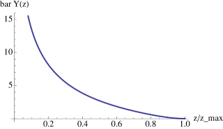
Figure 1: $\bar{Y}(z)$ in (40) using the Klebanov-Strassler metric.

Table 2: Geometric means $a^{(I)}_{\text{typ}}$ and $b^{(I)}_{\text{typ}}$ and the standard deviations of $\ln|a^{(I)}_{n_{1}n_{2}m_{1}\dots m_{I}}|$ and $\ln|b^{(I)}_{n_{1}n_{2}m_{1}\dots m_{I}}|$, $\sigma^{(I)}_{\ln a}$ and $\sigma^{(I)}_{\ln b}$, respectively, calculated numerically in a model (40) using the Klebanov-Strassler metric. Just like in Table 1, $\sigma^{(I)}$ in the 3rd and 5th columns are presented in the form of $\ln[\;\exp(\sigma^{(I)})\;]$.

	$\displaystyle{a^{(I)}_{\text{typ}}\left(\frac{4\pi}{\sqrt{2a_{\text{eff}}}}\Lambda_{\text{NDA}}z_{\text{max}}\cdot 1.5\right)^{-I}}$	$\sigma^{(I)}_{\ln a}$	$\displaystyle{b^{(I)}_{\text{typ}}\left(\frac{4\pi}{\sqrt{2a_{\text{eff}}}}\Lambda_{\text{NDA}}z_{\text{max}}\cdot 1.5\right)^{-I}}$	$\sigma^{(I)}_{\ln b}$
$I=1$	0.3	$\ln[2.]$	$\left(\frac{m_{1}}{\Lambda_{\text{NDA}}}\right)^{2}\times 0.3$	$\ln[3.]$
$I=2$	0.3	$\ln[1.]$	$\left(\frac{m_{1}}{\Lambda_{\text{NDA}}}\right)^{2}\times 0.2$	$\ln[4.]$
$I=3$	0.4	$\ln[2.]$	$\left(\frac{m_{1}}{\Lambda_{\text{NDA}}}\right)^{2}\times 0.2$	$\ln[4.]$
$I=4$	0.5	$\ln[2.]$	$\left(\frac{m_{1}}{\Lambda_{\text{NDA}}}\right)^{2}\times 0.2$	$\ln[3.]$

4 Summary

Our study based on gauge/string duality is summarized as follows: the NDA scaling rule does exist for the scalar glueballs dual to $\phi$ and $c$ fields, and the scaling factor is given by (31). The error of the scaling factor is within a factor two or so (0.8 for hard wall model and 1.5 for the model using the Klebanov-Strassler metric.) The uncertainty in the choice of $a_{\text{eff}}$ is also of the same order. The $N_{c}$ dependence of hadron couplings following from the large $N_{c}$ argument (and from string theory) is now generalized in the language of $a(z)$ function defined in holographic models, which roughly characterizes the degree of freedom in the dual theories. With this generalization, the NDA scaling rule can be applied also to some class of quiver gauge theories.

If we are to use the mass of the lightest (non-Nambu–Goldstone boson) hadron as the $\Lambda_{\rm NDA}$ mass scale in (1), the scaling factor comes out to be larger than the conventional one, by $(mz_{\rm max})$, which is about $5\sim 6$ in the two models we studied numerically. We can say that the (dimensionless) coefficients of hadron couplings are systematically larger than the conventional NDA ansatz, but alternatively, we can also say, by taking $\Lambda_{\rm NDA}\simeq 1/z_{\rm max}$, that the coefficients of hadron couplings are just as expected in the conventional NDA ansatz, and mass parameters are somewhat larger than naively expected from $\Lambda_{\rm NDA}$. We have nothing to say, however, about whether the large value of $mz_{\rm max}$ is a generic feature of hadrons from strongly coupled theories, or just happens to be a specific feature of the two models we studied.

So far, we are not sure whether coupling constants of any other hadrons have the NDA scaling rule, and if so, what are the NDA scaling factors. These are subjects in our future work.

References

- [1] A. Manohar and H. Georgi, Nucl. Phys. B 234, 189 (1984).
- [2] H. Georgi and L. Randall, Nucl. Phys. B 276, 241 (1986).
- [3] M. A. Luty, Phys. Rev. D 57, 1531 (1998) [hep-ph/9706235].
- [4] A. G. Cohen, D. B. Kaplan and A. E. Nelson, Phys. Lett. B 412, 301 (1997) [hep-ph/9706275].
- [5] H. Georgi, Phys. Lett. B 298, 187 (1993) [hep-ph/9207278]. [6]
- [6] E. Witten, Annals Phys. 128, 363 (1980).
- [7] J. M. Maldacena, Adv. Theor. Math. Phys. 2, 231 (1998) [Int. J. Theor. Phys. 38, 1113 (1999)] [hep-th/9711200].
- [8] S. S. Gubser, I. R. Klebanov and A. M. Polyakov, Phys. Lett. B 428, 105 (1998) [hep-th/9802109].
- [9] E. Witten, Adv. Theor. Math. Phys. 2, 253 (1998) [hep-th/9802150].
- [10] T. Sakai and S. Sugimoto, Prog. Theor. Phys. 113, 843 (2005) [hep-th/0412141].
- [11] T. Sakai and S. Sugimoto, Prog. Theor. Phys. 114, 1083 (2005) [hep-th/0507073].
- [12] W. Mueck and M. Prisco, JHEP 0404, 037 (2004) [hep-th/0402068].
- [13] S. Hong, S. Yoon and M. J. Strassler, JHEP 0604, 003 (2006) [hep-th/0409118].
- [14] S. Hong, S. Yoon and M. J. Strassler, hep-ph/0501197.
- [15] J. Erlich, E. Katz, D. T. Son and M. A. Stephanov, Phys. Rev. Lett. 95, 261602 (2005) [hep-ph/0501128].
- [16] N. J. Evans and J. P. Shock, Phys. Rev. D 70, 046002 (2004) [hep-th/0403279].
- [17] I. R. Klebanov and E. Witten, Nucl. Phys. B 536, 199 (1998) [hep-th/9807080].
- [18] J. P. Gauntlett, D. Martelli, J. Sparks and D. Waldram, Adv. Theor. Math. Phys. 8, 711 (2004) [hep-th/0403002].
- [19] S. Benvenuti, S. Franco, A. Hanany, D. Martelli and J. Sparks, JHEP 0506, 064 (2005) [hep-th/0411264].
- [20] E. Witten, Adv. Theor. Math. Phys. 2, 505 (1998) [hep-th/9803131].
- [21] J. Polchinski and M. J. Strassler, hep-th/0003136.
- [22] I. R. Klebanov and M. J. Strassler, JHEP 0008, 052 (2000) [hep-th/0007191].
- [23] J. M. Maldacena and C. Nunez, Phys. Rev. Lett. 86, 588 (2001) [hep-th/0008001].
- [24] A. Butti, M. Grana, R. Minasian, M. Petrini and A. Zaffaroni, JHEP 0503, 069 (2005) [hep-th/0412187].
- [25] Y. Kinar, E. Schreiber and J. Sonnenschein, Nucl. Phys. B 566, 103 (2000) [hep-th/9811192].
- [26] M. J. Duff, Class. Quant. Grav. 11, 1387 (1994) [hep-th/9308075].
- [27] S. S. Gubser, Phys. Rev. D 59, 025006 (1998) [hep-th/9807164].
- [28] M. Henningson and K. Skenderis, JHEP 9807, 023 (1998) [hep-th/9806087].
- [29] J. P. Gauntlett, D. Martelli, J. Sparks and S. -T. Yau, Commun. Math. Phys. 273, 803 (2007) [hep-th/0607080].
- [30] D. Z. Freedman, S. S. Gubser, K. Pilch and N. P. Warner, Adv. Theor. Math. Phys. 3, 363 (1999) [hep-th/9904017].
- [31] Z. Komargodski and A. Schwimmer, JHEP 1112, 099 (2011) [arXiv:1107.3987 [hep-th]].
- [32] J. Polchinski and M. J. Strassler, Phys. Rev. Lett. 88, 031601 (2002) [hep-th/0109174].
- [33] I. R. Klebanov and A. A. Tseytlin, Nucl. Phys. B 578, 123 (2000) [hep-th/0002159].
- [34] C. P. Herzog, I. R. Klebanov and P. Ouyang, hep-th/0205100.
- [35] P. Candelas and X. C. de la Ossa, Nucl. Phys. B 342, 246 (1990).