On moving-average models with feedback

Abstract

Moving average models, linear or nonlinear, are characterized by their short memory. This paper shows that, in the presence of feedback in the dynamics, the above characteristic can disappear.

, and

1 Introduction

Since the introduction by Slutsky [13], moving average models have played a significant role in time series analysis, especially in finance and economics. The models have been extended to include measurable (nonlinear) functions of independent and identically distributed random variables, representing unobservable and purely random impulses, for example, Robinson [12]. The characterizing feature of these models is the cut-off of the auto-covariance functions when they exist, implying that they are models of short memory. Another interesting feature of these models is the homogeneity of the random impulses, free from any feedback in the generating mechanism. Now, Slutsky developed these models in an economic context; the random impulses may correspond to unobservable political factors. In such a context, as well as in other contexts for which these models are relevant (e.g., business studies), it can be argued that feedback is often present: political decisions are often predicated on economic conditions. One simple way to incorporate feedback in these models is through the notion of thresholds, that is, on-off feedback controllers.

Since Tong [14] initiated the threshold notion in time series modelling, the notion has been extensively used in the literature, especially for the threshold autoregressive (TAR) or TAR-type models. For these models, some basic and probabilistic properties were given in Chan et al. [3] and Chan and Tong [4]. More related results can be found in An and Huang [1], Brockwell et al. [2], Chen and Tsay [5], Cline and Pu [6, 7], Ling [8], Ling et al. [9], Liu and Susko [10] and Lu [11], among others. A fairly comprehensive review of threshold models is available in Tong [15] and a selective survey of the history of threshold models is given by Tong [16].

However, most work to-date on the threshold model has primarily concentrated on the TAR or the TAR-type model. The threshold moving average (TMA) model, that is a moving average model with a simple on-off feedback control mechanism, has not attracted as much attention. As far as we know, only a few results are available for the TMA model. Brockwell et al. [2] investigated a threshold autoregressive and moving-average (TARMA) model and obtained a strictly stationary and ergodic solution to the model when the MA part does not contain any threshold component. Unfortunately, their TARMA model does not cover the TMA model as a special case. Using the Markov chain theory, Liu and Susko [10] provided the existence of the strictly stationary solution to the TMA model without any restriction on the coefficients. However, they neither gave an explicit form of the solution nor proved the ergodicity. A similar result can be found in Ling [8]. Ling et al. [9] gave a sufficient condition for the ergodicity of the solution for a first order TMA model under some restrictive conditions. These results have been extended to the first-order TMA model with more than two regimes. However, the uniqueness and the ergodicity of the solution are still open problems for higher-order TMA models.

In this paper, we use a different approach to study the TMA model without resorting to the Markov chain theory. Note that the TMA model involves a feedback control mechanism. An intuitive and simple idea is to seek a closed form of the solution in terms of the above mechanism, which is expressible as an indicator function. We can show that for the TMA model there always exists a unique strictly stationary and ergodic solution without any restriction on the coefficients of the TMA model. More importantly, for the first time in the literature, an explicit/closed form of the solution is derived. In addition, for the correlation structure, we show that the ACF (when it exists) of the TMA model typically does not cut off. In fact, it has a much richer structure. For example, it can exhibit almost long memory, although it generally decays at an exponential rate. Furthermore, the difference between the joint two-dimensional distribution and the corresponding product of its marginal distributions also decays to zero at an exponential rate as the lag tends to infinity.

The rest of the paper is organized as follows. Section 2 discusses the strict stationarity and ergodicity of the TMA model. Section 3 studies the asymptotic behaviour of the ACF of the TMA model and other correlation structure. We conclude in Section 4. All proofs of the theorems are relegated to the Appendix.

2 Stationarity and ergodicity of $\operatorname{TMA}(q)$ models

We first consider a $\operatorname{TMA}(q)$ model which satisfies the following equation:

$$y_{n}=\cases{\displaystyle\mu_{1}+e_{n}+\sum_{i=1}^{q}\phi_{i}e_{n-i},&\quad if $y_{n-d}\leq r$,\vspace*{2pt}\cr\displaystyle\mu_{2}+e_{n}+\sum_{i=1}^{q}\psi_{i}e_{n-i},&\quad if $y_{n-d}>r$,}$$ (1)

where $\{e_{n}\}$ is a sequence of i.i.d. random variables. Here, $q$ and $d$ are positive integers, $r\in\mathbb{R}$, the real line, is the threshold parameter, and $\mu_{1},\mu_{2},\phi_{i}$ and $\psi_{i}$, $i=1,\ldots,q$, are real coefficients.

For the sake of simplicity, we adopt the following notation:

$$U_{n}=\mathbbl{1}(a_{n}\leq r)\quad\mbox{and}\quad W_{n}=\mathbbl{1}(b_{n}\leq r)-\mathbbl{1}(a_{n}\leq r),$$

where $\mathbbl{1}(\cdot)$ is an indicator function,

$$a_{n}=\mu_{2}+e_{n}+\sum_{i=1}^{q}\psi_{i}e_{n-i}\quad\mbox{and}\quad b_{n}=\mu_{1}+e_{n}+\sum_{i=1}^{q}\phi_{i}e_{n-i}.$$ (2)

The following theorem gives the strict stationarity and ergodicity of model (1).

Theorem 2.1

Suppose that $\{e_{n}\}$ is a sequence of i.i.d. random variables with $\mathbb{P}(a_{n}\leq r,\allowbreak b_{n}\leq r)+\mathbb{P}(a_{n}>r,b_{n}>r)\not=0$. Then $y_{n}$ has a unique strictly stationary and ergodic solution expressed by

$$y_{n}=\mu_{2}+e_{n}+\sum_{i=1}^{q}\psi_{i}e_{n-i}+\Biggl{[}(\mu_{1}-\mu_{2})+\sum_{i=1}^{q}(\phi_{i}-\psi_{i})e_{n-i}\Biggr{]}\alpha_{n-d},\qquad\mbox{a.s.},$$

where

$$\alpha_{n-d}=\sum_{j=1}^{\infty}\Biggl{[}\Biggl{(}\prod_{s=1}^{j-1}W_{n-sd}\Biggr{)}U_{n-jd}\Biggr{]},\qquad\mbox{in $L^{1}$ and a.s.}\vspace*{-3pt}$$

If $e_{1}$ has a strictly and continuously positive density on $\mathbb{R}$ (e.g., normal, Student’s $t_{v}$ or double exponential distribution), then $\mathbb{P}(a_{n}\leq r,b_{n}\leq r)+\mathbb{P}(a_{n}>r,b_{n}>r)\not=0$. The basic idea for Theorem 2.1 is a direct and concrete expression in terms of $\mathbbl{1}(y_{n-d}\leq r)$, without resorting to the Markov chain theory. Theorem 2.1 shows that the $\operatorname{TMA}(q)$ model is always stationary and ergodic as is the $\operatorname{MA}(q)$ model.

3 The ACF of $\operatorname{TMA}(q)$ models

The ACF plays a crucial role in studying the correlation structure of weakly stationary time series. It is well known that for a causal $\operatorname{ARMA}(p,q)$ model, its ACF $\rho_{k}$ goes to zero at an exponential rate as $k$ diverges to infinity. The exact formula for ACF can be obtained although its closed form is not compact. However, for a general nonlinear time series model, it is rather difficult to obtain an exact formula for the ACF and to study the asymptotic behaviour. Additionally, the notion of memory, short or long, is closely associated with the ACF. One significant fact is that a causal $\operatorname{ARMA}(p,q)$ model is short-memory. For a general nonlinear time series model, due to its complicated structure, there is no universally accepted criterion for determining whether or not it is short-memory. As for some specific time series model, an ad hoc approach is usually adopted.

One important characteristic of the $\operatorname{MA}(q)$ model is that its ACF cuts off after lag $q$. Interestingly, this property is not generally inherited by the TMA model; this is not surprising theoretically because the TMA model involves some nonlinear feedback. Another interesting fact is that although a TMA model is generally short-memory, in some cases it can exhibit some almost long-memory phenomena; see Example 3.3. The following theorem characterizes the ACF of model (1).

Theorem 3.1

Suppose that the condition in Theorem 2.1 is satisfied and $\mathbb{E}|e_{1}|^{2}<\infty$. Then there exists a constant $\rho\in(0,1)$ such that $\rho_{k}=\mathrm{O}(\rho^{k})$.

Theorem 3.1 indicates that the TMA model (1) is short-memory. The next theorem describes the relationship between the two-dimensional joint distribution and the corresponding marginal distributions.

Theorem 3.2

Suppose that $\{e_{n}\}$ is i.i.d. random variables having a continuously, boundedly and strictly positive density. Then, for any $u,v\in\mathbb{R}$ and $k\geq 1$, there exists a constant $\rho\in(0,1)$ such that

$$|\mathbb{P}(y_{0}\leq u,y_{k}\leq v)-\mathbb{P}(y_{0}\leq u)\mathbb{P}(y_{k}\leq v)|=\mathrm{O}(\rho^{k}).\vspace*{-3pt}$$

Actually, Theorem 3.2 still holds for $\operatorname{Cov}(\mathbbl{1}(u_{1}<y_{0}\leq u_{2}),\mathbbl{1}(v_{1}<y_{k}\leq v_{2}))$ where $-\infty\leq u_{1}<u_{2}\leq\infty$ and $-\infty\leq v_{1}<v_{2}\leq\infty$. Next, we consider some special TMA models and study their ACFs as well as some other properties.

Example 3.1.

Suppose that $y_{n}$ is defined as

$$y_{n}=\cases{\mu_{1}+e_{n},&\quad if $y_{n-1}\leq r$,\cr\mu_{2}+e_{n},&\quad if $y_{n-1}>r$,}$$

where $\{e_{n}\}$ satisfies the condition in Theorem 2.1 with mean $0$ and finite variance $\sigma^{2}$.

This example can also be regarded as a special case of the TAR model, which was studied in Tong [15], Question 29, page 212. By calculation, we have the ACF of $\{y_{n}\}$

$$\rho_{k}=\frac{(\mu_{1}-\mu_{2})\lambda_{k}+(\mu_{1}-\mu_{2})^{2}\delta_{0}(1-\delta_{0})\beta^{k}}{\sigma^{2}+(\mu_{1}-\mu_{2})^{2}\delta_{0}(1-\delta_{0})}\qquad\mbox{for }k\geq 1,$$

where $\lambda_{k}=\mathbb{E}[e_{n-k}\mathbbl{1}(y_{n-1}\leq r)]$, $\beta=[G(r-\mu_{1})-G(r-\mu_{2})]\in(-1,1)$ and $\delta_{0}=G(r-\mu_{2})/\allowbreak[1-G(r-\mu_{1})+G(r-\mu_{2})]$. Here, $G(x)$ is the distribution function of $e_{1}$.

Clearly, the ACF does not possess the cut-off property except for $\mu_{1}=\mu_{2}$. Generally, $\rho_{k}$ decays exponentially since $\lambda_{k}=\mathrm{O}(\rho^{k})$ for some $\rho\in(0,1)$ by the proof of Theorem 3.2. In the nonlinear time series literature, the search for a nonlinear AR model with long memory has been largely in vain. Against this background, it is interesting to note that as $\mu_{1}\rightarrow\infty$ and $\mu_{2}\rightarrow-\infty$, $\rho_{k}$ can exhibit almost long memory in that $\rho_{k}$ can be made to decay arbitrarily slowly. Note that Example 3.1 can be driven by a white noise process with a thin tailed distribution. The skewness and the kurtosis of $y_{n}$ are also available explicitly and interesting. Specifically,

$$\mathrm{skewness}=\frac{\mathbb{E}e_{1}^{3}+(\mu_{1}-\mu_{2})^{3}(\delta_{0}-3\delta_{0}^{2}+2\delta_{0}^{3})}{[\sigma^{2}+(\mu_{1}-\mu_{2})^{2}\delta_{0}(1-\delta_{0})]^{3/2}}$$

and

$$\mathrm{kurtosis}=\frac{\mathbb{E}e_{1}^{4}+6\sigma^{2}(\mu_{1}-\mu_{2})^{2}\delta_{0}(1-\delta_{0})+(\mu_{1}-\mu_{2})^{4}(\delta_{0}-4\delta_{0}^{2}+6\delta_{0}^{3}-3\delta_{0}^{4})}{[\sigma^{2}+(\mu_{1}-\mu_{2})^{2}\delta_{0}(1-\delta_{0})]^{2}},$$

respectively. The impact of the threshold parameter $r$ is related to the bi-modality of the marginal density, which can be established by simple calculation. When $e_{1}$ is standard normal and $(\mu_{1},\mu_{2})=(4,-1)$, Figure 1 shows the skewness and the kurtosis of $y_{n}$ as functions of $r$.

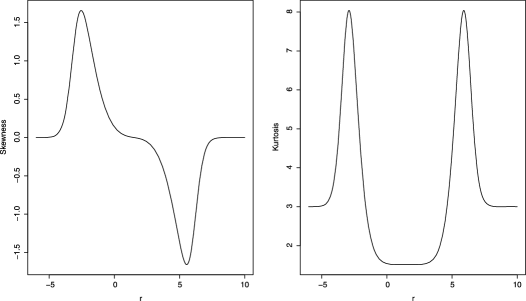
Figure 1: The skewness (left) and the kurtosis (right) of $y_{n}$ as functions of $r$ when $e_{1}$ is standard normal.

Example 3.2.

Suppose that $\{y_{n}\}$ follows a $\operatorname{TMA}(1)$ model without drift:

$$y_{n}=\cases{e_{n}+\phi e_{n-1},&\quad if $y_{n-2}\leq r$,\cr e_{n}+\psi e_{n-1},&\quad if $y_{n-2}>r$,}$$

where $\{e_{n}\}$ satisfies the condition in Theorem 2.1, having zero mean and finite variance.

After simple calculation, we have the ACF

$$\rho_{k}=\cases{\displaystyle\frac{\psi+(\phi-\psi)\varrho}{1+\psi^{2}+(\phi^{2}-\psi^{2})\varrho},&\quad if $k=1$,\vspace*{2pt}\cr 0,&\quad if $k\geq 1$,}$$

where $\varrho=\mathbb{P}(e_{2}+\psi e_{1}\leq r)/[\mathbb{P}(e_{2}+\phi e_{1}>r)+\mathbb{P}(e_{2}+\psi e_{1}\leq r)]\in[0,1)$.

This example shows that for some special $\operatorname{TMA}(q)$ model, the ACF may be cut off after lag $q$. In particular, if $\phi=\psi$, then the ACF coincides with that of the classical linear MA(1) model. Unfortunately, for general TMA models with $d\leq q$, there are no explicit expressions available for the ACFs due to the extremely complicated dependence of $y_{t-d}$ on $\{e_{t-j},d\leq j\leq q\}$. However, we can obtain the sample ACFs of TMA models by simulation.

Example 3.3.

Suppose that $\{y_{n}\}$ follows the $\operatorname{TMA}(1)$ model:

$$y_{n}=\cases{5+e_{n}+0.2e_{n-1},&\quad if $y_{n-1}\leq 0.5$,\cr-3+e_{n}+0.8e_{n-1},&\quad if $y_{n-1}>0.5$,}$$ (3)

where $\{e_{n}\}$ is i.i.d. standard normal.

This model produces a time series that mimics a unit root and long memory. In Figure 2, the sample ACF of model (3) decays slowly, although model (3) is stationary.

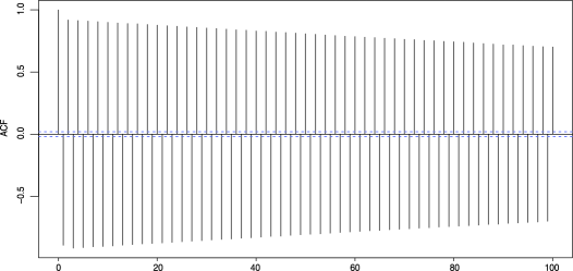
Figure 2: The sample ACFs of model (3).

4 Concluding remarks

Conventional moving average models, whether linear or nonlinear, assume absence of any feedback control mechanism. This paper shows that the introduction of simple feedback can enrich the structure of moving average models. For example, their ACF need not cut off but can now exhibit (near) long memory. Their distributions can be leptokurtic even when driven by Gaussian white noise. In nonlinear time series modeling, moving average models have been overshadowed by autoregressive models. Our study suggests that, by introducing a simple feedback mechanism, the notion of moving average possesses some unexpected properties beyond the shadow.

Appendix A Proofs of theorems

A.1 Proof of Theorem 2.1

From model $(\ref{p})$, $\mathbbl{1}(y_{n}\leq r)=U_{n}+W_{n}\mathbbl{1}(y_{n-d}\leq r).$ Iterating $k\geq 1$ steps, we have

$$\mathbbl{1}(y_{n}\leq r)=\sum_{j=0}^{k-1}\Biggl{[}\Biggl{(}\prod_{s=0}^{j-1}W_{n-sd}\Biggr{)}U_{n-jd}\Biggr{]}+\Biggl{(}\prod_{i=0}^{k-1}W_{n-id}\Biggr{)}\mathbbl{1}(y_{n-kd}\leq r)$$

with the convention $\prod_{0}^{-1}=1$. Let

$$\alpha_{n,k}=\sum_{j=0}^{k-1}\Biggl{[}\Biggl{(}\prod_{s=0}^{j-1}W_{n-sd}\Biggr{)}U_{n-jd}\Biggr{]}.$$

For given $d$ and $q$, there exists a unique nonnegative integer $m$ such that $md<\max(d,q+1)\leq(m+1)d$. Let $\delta=\mathbb{E}|W_{1}|$. Under the condition in Theorem 2.1, it is not difficult to prove that $0\leq\delta<1$. Observing that both $\{U_{n}\}$ and $\{W_{n}\}$ are $q$-dependent sequences, we can extract an independent subsequence $\{W_{n-j(m+1)d},j=0,1,\ldots,[\frac{k-1}{m+1}]\}$ from the sequence $\{W_{n-id},i=0,1,2,\ldots,k-1\}$, where $[a]$ denotes the integral part of $a$. Since $|U_{n}|\leq 1$ and $|W_{n}|\leq 1$, it yields that

$$\mathbb{E}\Biggl{|}\Biggl{(}\prod_{i=0}^{k-1}W_{n-id}\Biggr{)}U_{n-kd}\biggr{|}\leq(\mathbb{E}|W_{1}|)^{[(k-1)/(m+1)]},$$

implying

$$\sum_{j=1}^{\infty}\mathbb{E}\Biggl{|}\Biggl{(}\prod_{i=0}^{j-1}W_{n-id}\Biggr{)}U_{n-jd}\Biggr{|}\leq\sum_{j=1}^{\infty}\delta^{[(j-1)/(m+1)]}=(m+1)\sum_{k=0}^{\infty}\delta^{k}<\infty.$$

Using the above inequalities, we can prove that $\mathbb{E}|\alpha_{n,s}-\alpha_{n,t}|\rightarrow 0$ as $s,t\rightarrow\infty$ for each fixed $n$. By the Cauchy criterion, $\alpha_{n,k}$ converges in $L^{1}$ as $k\rightarrow\infty$. Write the limit as

$$\alpha_{n}=\sum_{j=0}^{\infty}\Biggl{[}\Biggl{(}\prod_{s=0}^{j-1}W_{n-sd}\Biggr{)}U_{n-jd}\Biggr{]}.$$

Applying the inequalities above again, it is easy to get

$$\sum_{k=1}^{\infty}\mathbb{E}|\alpha_{n,k}-\alpha_{n}|\leq\sum_{k=1}^{\infty}\sum_{j=k}^{\infty}\delta^{[(j-1)/(m+1)]}<\infty,$$

yielding that

$$\lim_{k\rightarrow\infty}\alpha_{n,k}=\alpha_{n},\qquad\mbox{in $L^{1}$ and a.s.}$$

Furthermore, recall that $U_{n}=\mathbbl{1}(a_{n}\leq r)$ and $W_{n}=\mathbbl{1}(b_{n}\leq r)-\mathbbl{1}(a_{n}\leq r)$, where $a_{n}$ and $b_{n}$ are defined in (2), we have the iterative sequence: $\alpha_{n,1}=U_{n}$ and

$$\alpha_{n,k}=U_{n}+W_{n}\alpha_{n-d,k-1}=(1-\alpha_{n-d,k-1})\mathbbl{1}(a_{n}\leq r)+\alpha_{n-d,k-1}\mathbbl{1}(b_{n}\leq r)$$

for each $n$ and $k\geq 1$. Note that $\alpha_{n,k}$ and $\alpha_{n-d,k}$ have the same distribution for fixed $k$ since the error $\{e_{i}\}$ is i.i.d. By induction over $k$, we have that $\alpha_{n,k}$ only takes two values 0 and 1 a.s. since $\alpha_{n,1}$ only takes 0 and 1. Thus, $\alpha_{n}$ at most takes two values 0 and 1 a.s., namely, $\alpha_{n}=\mathbbl{1}(\alpha_{n}=1)$ a.s. Define a new sequence $\{S_{n}\}$

$$S_{n}=\mu_{2}+e_{n}+\sum_{i=1}^{q}\psi_{i}e_{n-i}+\Biggl{[}(\mu_{1}-\mu_{2})+\sum_{i=1}^{q}(\phi_{i}-\psi_{i})e_{n-i}\Biggr{]}\alpha_{n-d}.$$

By simple calculation, we have

$$\mathbbl{1}(S_{n}\leq r) = \mathbbl{1}(a_{n}\leq r)\mathbbl{1}(\alpha_{n-d}=0)+\mathbbl{1}(b_{n}\leq r)\mathbbl{1}(\alpha_{n-d}=1)$$

$$= U_{n}+W_{n}\mathbbl{1}(\alpha_{n-d}=1)$$

$$= U_{n}+W_{n}\alpha_{n-d}=\alpha_{n},\qquad\mbox{a.s.}$$

Hence,

$$S_{n}=\mu_{2}+e_{n}+\sum_{i=1}^{q}\psi_{i}e_{n-i}+\Biggl{[}(\mu_{1}-\mu_{2})+\sum_{i=1}^{q}(\phi_{i}-\psi_{i})e_{n-i}\Biggr{]}\mathbbl{1}(S_{n-d}\leq r),\qquad\mbox{a.s.}$$

Thus, $\{S_{n}\}$ is the solution of model (2.1) which is strictly stationary and ergodic.

To uniqueness, suppose that $\tilde{S}_{n}$ is a solution to model (1), then

$$\mathbbl{1}(\tilde{S}_{n}\leq r)=U_{n}+W_{n}\mathbbl{1}(\tilde{S}_{n-d}\leq r).$$

Iterating the above equation, one can get for $k\geq 1$

$$\mathbbl{1}(\tilde{S}_{n}\leq r)=\alpha_{n,k}+\Biggl{(}\prod_{i=0}^{k-1}W_{n-id}\Biggr{)}\mathbbl{1}(\tilde{S}_{n-kd}\leq r).$$

We can show that the second term of the previous equation converges to zero a.s. Thus, we have $\mathbbl{1}(\tilde{S}_{n}\leq r)=\alpha_{n}$ a.s. Therefore,

$$\tilde{S}_{n}=\mu_{2}+e_{n}+\sum_{i=1}^{q}\psi_{i}e_{n-i}+\Biggl{[}(\mu_{1}-\mu_{2})+\sum_{i=1}^{q}(\phi_{i}-\psi_{i})e_{n-i}\Biggr{]}\alpha_{n-d},\qquad\mbox{a.s.},$$

that is, $\tilde{S}_{n}=S_{n}$ a.s. The proof is complete.

A.2 Proof of Theorem 3.1

The notations $a_{n}$ and $b_{n}$ are defined by (2), $m$ and $\delta$ are the same as those in the proof of Theorem 2.1. From Theorem 2.1, we have $y_{n}=a_{n}+(b_{n}-a_{n})\alpha_{n-d}$. For $n\geq(m+2)d+q$, we decompose $\alpha_{n-d}$ into two parts

$$\alpha_{n-d} = \sum_{j=1}^{[(n-q)/d]-1}\Biggl{[}\Biggl{(}\prod_{s=1}^{j-1}W_{n-sd}\Biggr{)}U_{n-jd}\Biggr{]}+\sum_{j=[(n-q)/d]}^{\infty}\Biggl{[}\Biggl{(}\prod_{s=1}^{j-1}W_{n-sd}\Biggr{)}U_{n-jd}\Biggr{]}$$

$$\equiv I_{1}+I_{2}.$$

Clearly, $I_{1}\in\mathcal{F}_{d}^{n-d}$ and $I_{2}\in\mathcal{F}_{-\infty}^{n-d}$, where $\mathcal{F}_{m}^{n}=\sigma(e_{m},\ldots,e_{n})$. By calculation, we have for $n\geq(m+2)d+q$

$$|\operatorname{Cov}(y_{0},y_{n})| \leq \sum_{j=[(n-q)/d]}^{\infty}\Biggl{[}\mathbb{E}\Biggl{(}\prod_{s=1}^{j-1}|W_{n-sd}|\Biggr{)}\Biggr{]}^{1/2}[\mathbb{E}(b_{n}-a_{n})^{2}(y_{0}-\mathbb{E}y_{0})^{2}]^{1/2}$$

$$\leq \sum_{j=[(n-q)/d]}^{\infty}\sqrt{\delta}^{[(j-1)/(m+1)]}[\mathbb{E}(b_{n}-a_{n})^{2}]^{1/2}[\mathbb{E}(y_{0}-\mathbb{E}y_{0})^{2}]^{1/2}$$

$$\leq \frac{H(m+1)}{1-\sqrt{\delta}}\sqrt{\delta}^{[(n-q-d)/(d(m+1))]-1}$$

by Hölder’s inequality, the boundedness of $W_{n}$ and $U_{n}$, and the independence of $\{b_{n},a_{n}\}$ and $y_{0}$, where

$$H=\Biggl{[}|\mu_{1}-\mu_{2}|+(\mathbb{E}e_{1}^{2})^{1/2}\sum_{i=1}^{q}|\phi_{i}-\psi_{i}|\Biggr{]}\Biggl{[}|\mu_{1}|+|\mu_{2}|+(\mathbb{E}e_{1}^{2})^{1/2}\sum_{i=1}^{q}(|\phi_{i}|+|\psi_{i}|)\Biggr{]}.$$

Thus, the conclusion holds.

A.3 Proof of Theorem 3.2

Let $x_{n}=a_{n}+(b_{n}-a_{n})I_{1}$. Then $y_{n}-x_{n}=(b_{n}-a_{n})I_{2}$. Clearly, $x_{n}\in\mathcal{F}_{d}^{n}$ and $\mathbb{E}|y_{n}-x_{n}|=\mathrm{O}(\rho^{n})$ for large enough $n$, where $\rho\in(0,1)$. So, using the independence of $x_{n}$ and $y_{0}$, for large enough $n$, we have

$$|\mathbb{P}(y_{0}\leq u,y_{n}\leq v)-\mathbb{P}(y_{0}\leq u)\mathbb{P}(y_{n}\leq v)|$$

$$\quad=|\mathbb{E}\{[\mathbbl{1}(y_{n}\leq v)-\mathbbl{1}(x_{n}\leq v)][\mathbbl{1}(y_{0}\leq u)-\mathbb{E}\mathbbl{1}(y_{0}\leq u)]\}|$$

$$\quad\leq\mathbb{E}|\mathbbl{1}(y_{n}\leq v)-\mathbbl{1}(x_{n}\leq v)|.$$

On noting the independence between $e_{n}$ and $\bar{e}_{n-1}$, where $\bar{e}_{n-1}=\mu_{2}+\sum_{i=1}^{q}\psi_{i}e_{n-i}+(b_{n}-a_{n})\alpha_{n-d}$, the density of $y_{n}$ is $f_{y}(x)=\int_{\mathbb{R}}h(x-y)\,\mathrm{d}G_{\bar{e}}(y)$, where $h(x)$ is the density function of $e_{1}$ and $G_{\bar{e}}(y)$ is the distribution function of $\bar{e}_{n-1}$. On using the property of convolution, $f_{y}(x)$ is continuous and bounded. Write $\|f_{y}\|_{\infty}=\max\{|f_{y}(x)|\colon\ x\in\mathbb{R}\}$. On the one hand, using the following inequality

$$|\mathbbl{1}(x\leq t)-\mathbbl{1}(y\leq t)|\mathbbl{1}(|x-y|\leq\varepsilon)\leq\mathbbl{1}(t-\varepsilon\leq x\leq t+\varepsilon),$$

we can get

$$\mathbb{E}[|\mathbbl{1}(y_{n}\leq v)-\mathbbl{1}(x_{n}\leq v)|\mathbbl{1}(|y_{n}-x_{n}|\leq\varepsilon)]\leq\mathbb{P}(v-\varepsilon\leq y_{n}\leq v+\varepsilon)\leq 2\|f_{y}\|_{\infty}\varepsilon.$$

On the other hand, using Markov’s inequality, we have

$$\mathbb{E}\{|\mathbbl{1}(y_{n}\leq v)-\mathbbl{1}(x_{n}\leq v)|\mathbbl{1}(|y_{n}-x_{n}|>\varepsilon)\}\leq\mathbb{E}\mathbbl{1}(|y_{n}-x_{n}|>\varepsilon)\}\leq\varepsilon^{-1}\mathbb{E}|y_{n}-x_{n}|.$$

Choosing $\varepsilon=\mathrm{O}(\rho^{n/2})$, we can obtain

$$|\mathbb{P}(y_{0}\leq u,y_{n}\leq v)-\mathbb{P}(y_{0}\leq u)\mathbb{P}(y_{n}\leq v)|=\mathrm{O}(\rho^{n/2}).$$

Hence, the result holds.

References

- [1] {barticle}[mr] \bauthor\bsnmAn, \bfnmH. Z.\binitsH.Z. &\bauthor\bsnmHuang, \bfnmF. C.\binitsF.C. (\byear1996). \btitleThe geometrical ergodicity of nonlinear autoregressive models. \bjournalStatist. Sinica \bvolume6 \bpages943–956. \bidissn=1017-0405, mr=1422412 \endbibitem
- [2] {barticle}[mr] \bauthor\bsnmBrockwell, \bfnmPeter J.\binitsP.J., \bauthor\bsnmLiu, \bfnmJian\binitsJ. &\bauthor\bsnmTweedie, \bfnmRichard L.\binitsR.L. (\byear1992). \btitleOn the existence of stationary threshold autoregressive moving-average processes. \bjournalJ. Time Ser. Anal. \bvolume13 \bpages95–107. \biddoi=10.1111/j.1467-9892.1992.tb00096.x, issn=0143-9782, mr=1165659 \endbibitem
- [3] {barticle}[mr] \bauthor\bsnmChan, \bfnmK. S.\binitsK.S., \bauthor\bsnmPetruccelli, \bfnmJoseph D.\binitsJ.D., \bauthor\bsnmTong, \bfnmH.\binitsH. &\bauthor\bsnmWoolford, \bfnmSamuel W.\binitsS.W. (\byear1985). \btitleA multiple-threshold AR model. \bjournalJ. Appl. Probab. \bvolume22 \bpages267–279. \bidissn=0021-9002, mr=0789351 \endbibitem
- [4] {barticle}[mr] \bauthor\bsnmChan, \bfnmK. S.\binitsK.S. &\bauthor\bsnmTong, \bfnmH.\binitsH. (\byear1985). \btitleOn the use of the deterministic Lyapunov function for the ergodicity of stochastic difference equations. \bjournalAdv. in Appl. Probab. \bvolume17 \bpages666–678. \biddoi=10.2307/1427125, issn=0001-8678, mr=0798881 \endbibitem
- [5] {barticle}[mr] \bauthor\bsnmChen, \bfnmRong\binitsR. &\bauthor\bsnmTsay, \bfnmRuey S.\binitsR.S. (\byear1991). \btitleOn the ergodicity of processes. \bjournalAnn. Appl. Probab. \bvolume1 \bpages613–634. \bidissn=1050-5164, mr=1129777 \endbibitem
- [6] {barticle}[mr] \bauthor\bsnmCline, \bfnmDaren B. H.\binitsD.B.H. &\bauthor\bsnmPu, \bfnmHuay-min H.\binitsH.m.H. (\byear1999). \btitleGeometric ergodicity of nonlinear time series. \bjournalStatist. Sinica \bvolume9 \bpages1103–1118. \bidissn=1017-0405, mr=1744827 \endbibitem
- [7] {barticle}[mr] \bauthor\bsnmCline, \bfnmDaren B. H.\binitsD.B.H. &\bauthor\bsnmPu, \bfnmHuay-Min H.\binitsH.M.H. (\byear2004). \btitleStability and the Lyapounov exponent of threshold AR-ARCH models. \bjournalAnn. Appl. Probab. \bvolume14 \bpages1920–1949. \biddoi=10.1214/105051604000000431, issn=1050-5164, mr=2099657 \endbibitem
- [8] {barticle}[mr] \bauthor\bsnmLing, \bfnmShiqing\binitsS. (\byear1999). \btitleOn the probabilistic properties of a double threshold ARMA conditional heteroskedastic model. \bjournalJ. Appl. Probab. \bvolume36 \bpages688–705. \bidissn=0021-9002, mr=1737046 \endbibitem
- [9] {barticle}[mr] \bauthor\bsnmLing, \bfnmShiqing\binitsS., \bauthor\bsnmTong, \bfnmHowell\binitsH. &\bauthor\bsnmLi, \bfnmDong\binitsD. (\byear2007). \btitleErgodicity and invertibility of threshold moving-average models. \bjournalBernoulli \bvolume13 \bpages161–168. \biddoi=10.3150/07-BEJ5147, issn=1350-7265, mr=2307400 \endbibitem
- [10] {barticle}[mr] \bauthor\bsnmLiu, \bfnmJian\binitsJ. &\bauthor\bsnmSusko, \bfnmEd\binitsE. (\byear1992). \btitleOn strict stationarity and ergodicity of a nonlinear ARMA model. \bjournalJ. Appl. Probab. \bvolume29 \bpages363–373. \bidissn=0021-9002, mr=1165221 \endbibitem
- [11] {barticle}[mr] \bauthor\bsnmLu, \bfnmZudi\binitsZ. (\byear1998). \btitleOn the geometric ergodicity of a non-linear autoregressive model with an autoregressive conditional heteroscedastic term. \bjournalStatist. Sinica \bvolume8 \bpages1205–1217. \bidissn=1017-0405, mr=1666249 \endbibitem
- [12] {barticle}[mr] \bauthor\bsnmRobinson, \bfnmP. M.\binitsP.M. (\byear1977). \btitleThe estimation of a nonlinear moving average model. \bjournalStochastic Process. Appl. \bvolume5 \bpages81–90. \bidissn=0304-4149, mr=0428654 \endbibitem
- [13] {bmisc}[auto:STB—2011/09/12—07:03:23] \bauthor\bsnmSlutsky, \bfnmE.\binitsE. (\byear1927). \bhowpublishedThe summation of random causes as the source of cyclic processes. Voprosy Koniunktury 3 34–64. {English translation in Econometrika 5 105–146.}. \endbibitem
- [14] {bincollection}[auto:STB—2011/09/12—07:03:23] \bauthor\bsnmTong, \bfnmHowell\binitsH. (\byear1978). \btitleOn a thresold model. In \bbooktitlePattern Recognition and Signal Processing (\beditor\bfnmChi Hau\binitsC.H. \bsnmChen, ed.) \bpages575–586. \baddressAmsterdam: \bpublisherSijthoff and Noordhoff. \endbibitem
- [15] {bbook}[mr] \bauthor\bsnmTong, \bfnmHowell\binitsH. (\byear1990). \btitleNonlinear Time Series: A Dynamical System Approach. \bseriesOxford Statistical Science Series \bvolume6. \baddressNew York: \bpublisherOxford Univ. Press. \bidmr=1079320 \endbibitem
- [16] {bmisc}[auto:STB—2011/09/12—07:03:23] \bauthor\bsnmTong, \bfnmH.\binitsH. (\byear2011). \bhowpublishedThreshold models in time series analysis – 30 years on. Stat. Interface 4 107–118. \endbibitem