Real-time Quantum evolution in the Classical approximation and beyond

Abstract

With the goal in mind of deriving a method to compute quantum corrections for the real-time evolution in quantum field theory, we analyze the problem from the perspective of the Wigner function. We argue that this provides the most natural way to justify and extend the classical approximation. A simple proposal is presented that can allow to give systematic quantum corrections to the evolution of expectation values and/or an estimate of the errors committed when using the classical approximation. The method is applied to the case of a few degrees of freedom and compared with other methods and with the exact quantum results. An analysis of the dependence of the numerical effort involved as a function of the number of variables is given, which allow us to be optimistic about its applicability in a quantum field theoretical context.

I Introduction

Quantum Phenomena underlie most of Modern Physics. Alongside it brings in the necessity of dealing with complex functions and interference phenomena. In particular, determining the time evolution of a quantum system is relevant for many areas of Physics. When a large number of degrees of freedom is involved, numerical methods based on the integration of the Schroedinger equation fail. This, however, is the typical situation in Quantum Field Theory (QFT).

When computing expectation values of operators in the vacuum or in the equilibrium state, one can use the path-integral approach. Furthermore, in the computation of the Wick-rotated Green functions of the theory, the complex quantum weight of each trajectory is transformed into a positive-definite probability weight. This allows the use of efficient standard importance sampling techniques, such as the Metropolis algorithm or other Monte Carlo techniques. This information allows the extraction of the spectrum and other properties of the theory. The same applies when studying Quantum Field Theory at equilibrium. However, even in this situation, there are important exceptions in which the weights are not positive definite and the standard Monte Carlo methods fail. This is often referred as the sign problem. One example occurs in certain Quantum Field theories, as QCD, at finite chemical potential. Many methods have been devised to obtain relevant information in this situation, meeting partial success deForcrand:2009ys . However, it is generally accepted that, despite the efforts, no fully satisfactory solution has been found. This is particularly unwelcome, since full-proof predictions in certain areas of Physics, which are of great relevance and timeliness (such as Heavy Ion collisions) are lacking.

When studying the quantum evolution away from equilibrium or from a initial state which is not an eigenstate of the Hamiltonian the situation is even more severe. In this context, path integral methods for time-dependent expectation values follow from the Schwinger-Keldysh formalism Schwinger:1960qe Keldysh:1964ud . This allows systematic perturbative calculations. However, non-perturbative phenomena are often crucial and we lack an efficient numerical computational method to deal with this situation (for a review see Ref. Berges:2004yj ).

This problem arises in different areas of Physics such as Nuclear Physics, Quantum Chemistry, Quantum Optics, etc. One of these areas is Cosmology, which actually triggered the interest of the present authors in the problem. Quantum fluctuations play a role at different instances in the early Universe. One such case is at the inflationary era, by generating the density fluctuations which act as sources for the anisotropies of the cosmic background radiation and the formation of structures. Many authors argued that the fluctuations develop from quantum to classical, and can be treated as classical at late times Guth:1985ya -Koksma:2011dy . Another interesting epoch which depends crucially on the understanding of the quantum evolution of a quantum field theory, is that of preheating and reheating after inflation Kofman:1994rk -Greene:1997fu . Properties of the present Universe, such as baryon number density, gravitational waves or magnetic field remnants, might depend upon this dynamics. Obtaining reliable estimates demand an appropriate treatment of the quantum field theory evolution from an initial state after inflation to the fully thermalized reheated Universe. To estimate these effects, several authors Khlebnikov:1996mc -DiazGil:2008tf have employed the so-called classical approximation (For a somewhat different context see also Refs. Aarts:2001yn -Aarts:2001yx ). This consists on treating certain modes of the quantum fields as random fields with deterministic dynamics given by the classical equations of motion of the system. The randomness is imprinted in the initial conditions of the fields, often determined by a particularly simple initial quantum state. The authors who employ the classical approximation, often present arguments to determine which modes can indeed be treated as classical and those that cannot, leading to different types of initial conditions in both cases. The last point is crucial since in Quantum Field Theory there are ultraviolet divergences. An appropriate treatment has to deal with them through Renormalization.

The present work originated with the goal of determining the region of validity of the classical approximation, estimating the size of the errors induced by it, and hopefully even obtaining a way to go beyond it, by incorporating quantum corrections to the results. For that purpose we have started by analyzing simple quantum systems with very few degrees of freedom whose quantum evolution can be obtained by numerical integration of the Schroedinger equation. The initial conditions and the type of Hamiltonians considered are inspired by the field theoretical and cosmological applications. Thus, we focus upon quartic interactions and gaussian or thermal initial conditions.

In all cases we have compared the results obtained by the classical approximation with the exact quantum evolution. Furthermore, we have also studied the results obtained with different proposals for incorporating quantum corrections, limiting ourselves to those that have any hope of being applicable to the quantum field theoretical case. In particular, a very interesting technique is the two-particle irreducible effective action supplemented with a certain truncation of the number of diagrams involved (2PI method) PhysRev.127.1391 - Cornwall:1974vz . This truncation can be based on the loop expansion or on the 1/N expansion Berges:2001fi . The latter behaves in a more stable fashion and has been used in our analysis. We remark that the traditional Hartree method can be considered a particular case of the 2PI method PhysRevD.36.3114 -PhysRevD.65.045012 . In any case the method is limited to the determination of the quantum evolution of certain observables, such as the 2-point correlation function of the system (see Ref. Berges:2004yj for a more complete list of early references on the subject).

Another technique which has been recently applied in the context of Quantum Field Theory is the complex Langevin method Klauder:1983zm -Berges:2005yt . This is based on complexifying the fields and studying the dynamics of the field trajectories induced by a Langevin equation in an additional Langevin-time variable with a purely imaginary drift term. Instabilities are often found in the numerical integration of this equation, although authors have given several recipes to avoid them Aarts:2009dg . Furthermore, good results have been reported in certain cases Aarts:2009uq -Aarts:2011ax , so that we thought it was very interesting to apply it to our examples. Unfortunately, we seem to be in a situation in which convergence to the right solution does not apply. This question deserves future study.

In parallel to the tests explained before, we present a method to quantify and incorporate quantum effects based upon the Wigner function Wigner:1932eb . This is a pseudo-distribution function, whose expectation values give us the matrix elements of Weyl-ordered products of operators in the quantum state of the system. The function is real, but not positive definite (see Ref. Hillery:1983ms for an account of all its properties). The Wigner function satisfies an evolution equation Moyal:1949sk in time, which determines the time-dependence of all these expectation values. One of the advantages of this method, is that it is particularly simple to see what is the meaning of the classical evolution and what is the nature of quantum corrections. This will be explained in the next section. This observation is not novel, and has led different researchers in different fields to focus on the Wigner function and its evolution equation when attempting to describe quantum evolution Remler:1975fm -Kunihiro:2008gv . One example, is in Nuclear Physics where several authors Bonasera:1993zz John:2007zz have developed methodologies which are very similar in spirit to our goal (see also Remler_1987 ). Unfortunately, the detailed techniques seem hard to extend to a large number of degrees and thus to Quantum field theory. In our particular proposal we have dedicated some time to study the way in which the numerical effort involved scales with the number of degrees of freedom. A power-like growth is acceptable even if it involves an enormous computational effort. Experience teaches us that the development of computer technology and algorithms will diminish the load in due time. An exponential growth is a killer. Our results presented below are promising and seem to allow the computation of quantum corrections in typical situations relevant for cosmological applications. This will be addressed in a future paper of the present authors. The present paper is to be considered a pilot study, in which we have the advantage of knowing what the exact quantum result is. The full field theoretical case demands a much higher computational cost, in addition with the necessity of dealing with issues as renormalization, as mentioned previously.

For a more complete account of the literature we should mention the work of Mrowczynski:1994nf , in which the authors advocate the use of the Wigner function evolution equation in Quantum Field Theory and give ideas on possible techniques to obtain an explicit calculation of the quantum corrections in this setting.

We conclude this section by describing the lay-out of the paper. In the next section we review the definition of the Wigner function and derive its time-evolution equation. We also explain the meaning of the classical approximation in this context. The following section explains how, in trying to derive the quantum Liouville equation as a Fokker-Planck equation associated to a Langevin process, the non-positive definite character leads to pathological properties of the stochastic force. With this idea in mind, in Section IV we present a method to relate the equation to a regular markovian process for which standard sample methods can be applied. This together with a certain coarse-graining approximation allows to set up a procedure to calculate systematic quantum corrections to the evolution in powers of $\hbar^{2}$. In the following section, we study several simple cases for which we analyze the accuracy of the classical approximation, the truncated 2PI method and our proposal of the previous section. Special attention is paid to estimate the capacity of the method to deal with discretized lattice approximations to quantum field theory. In the concluding section, we summarize our results and discuss the advantages and limitations of our proposal.

II The Wigner function evolution equation

In Quantum Mechanics the expectation values of Weyl-ordered products of operators can be computed in terms of the Wigner function $W(x,p,t)$ as followsWigner:1932eb Hillery:1983ms :

$$\langle\Psi|f_{W}(Q,P)|\Psi\rangle=\int\frac{dx\,dp}{\hbar}f(x,p)\,W(x,p,t)$$ (1)

where $f_{W}(Q,P)$ means a Weyl-ordered product of position and momentum operators, whose classical limit is $f(x,p)$. For a pure state, given the wave function $\Psi(x,t)$, the expression of the Wigner function is

$$W(x,p,t)=\int\frac{dy}{2\pi}\,\Psi^{*}(x+y/2,t)\Psi(x-y/2,t)\,e^{ipy/\hbar}$$ (2)

This can be extended to mixed states associated to a density matrix $\mathbf{\rho}(t)$ as follows:

$$W(x,p,t)=\int\frac{dy}{2\pi}\,\langle x-y/2|\mathbf{\rho}(t)|x+y/2\rangle\,e^{ipy/\hbar}$$ (3)

In both cases the Wigner function is real but not necessarily positive definite.

The Wigner function satisfies an evolution equation in time which depends on the form of the potential. Here we will derive it for the case of Hamiltonian of the form

$$H=\frac{p^{2}}{2m}+V(x)$$ (4)

The corresponding Schroedinger equation satisfied by the wave function is

$$i\partial_{0}\Psi(x,t)=-\frac{\hbar}{2m}\frac{\partial^{2}}{\partial x^{2}}\Psi(x,t)+\frac{V(x)}{\hbar}\Psi(x,t)$$ (5)

From this equation, using the relation Eq. 2, one can derive the equation followed by the Wigner function:

$$\partial_{0}W(x,p,t) =\frac{i\hbar}{2m}\int\frac{dy}{2\pi}\,e^{ipy/\hbar}\left(\Psi^{*}(x+\frac{y}{2},t)\frac{\partial^{2}\Psi(x-\frac{y}{2},t)}{\partial x^{2}}-\frac{\partial^{2}\Psi^{*}(x+\frac{y}{2},t)}{\partial x^{2}}\Psi(x-\frac{y}{2},t)\right)+$$ (6)

$$+\frac{i}{\hbar}\int\frac{dy}{2\pi}\,\Psi^{*}(x+\frac{y}{2},t)\,\Psi(x-\frac{y}{2},t)\,e^{ipy/\hbar}(V(x+\frac{y}{2})-V(x-\frac{y}{2}))\>\>\>$$

One can transform the right hand side in an obvious way and obtain

$$\int\frac{dy}{2\pi}\,e^{ipy/\hbar}\left(\frac{-i\hbar}{m}\frac{\partial^{2}}{\partial x\partial y}+\frac{i}{\hbar}\left(V(x+\frac{y}{2})-V(x-\frac{y}{2})\right)\right)\Psi^{*}(x+\frac{y}{2},t)\,\Psi(x-\frac{y}{2},t)$$

Integrating by parts one can substitute $\frac{\partial}{\partial y}$ by $-ip/\hbar$. On the other hand, the factors of y can be replaced by $-i\hbar\frac{\partial}{\partial p}$. We end up with the equation

$$\partial_{0}W(x,p,t)=-\frac{p}{m}\frac{\partial W(x,p,t)}{\partial x}+\frac{i}{\hbar}\left(V(x-\frac{i\hbar}{2}\frac{\partial}{\partial p})-V(x+\frac{i\hbar}{2}\frac{\partial}{\partial p})\right)W(x,p,t)$$ (7)

This equation is well-known Moyal:1949sk and receives several names in the literature: Moyal equation or quantum Liouville equation.

Let us now restrict to a potential of the form

$$V(x)=\frac{\mu^{2}}{2}x^{2}+\frac{\lambda}{4!}x^{4}$$ (8)

The operator involving $V$ can be expanded to give

$$V^{\prime}(x)\frac{\partial}{\partial p}-\frac{\hbar^{2}}{24}V^{\prime\prime\prime}(x)\frac{\partial^{3}}{\partial p^{3}}$$ (9)

Then, we are finally led to an equation of the form:

$$\partial_{0}W(x,p,t)=-\frac{p}{m}\hskip 1.0pt\frac{\partial W(x,p,t)}{\partial x}+V^{\prime}(x)\hskip 1.0pt\frac{\partial W(x,p,t)}{\partial p}-\frac{\lambda\hbar^{2}x}{24}\hskip 1.0pt\frac{\partial^{3}W(x,p,t)}{\partial p^{3}}$$ (10)

Notice that the first two terms do not contain $\hbar$. As a matter of fact, if we neglect the last term, the solution to this partial differential equation is very simple. It is given by

$$W_{0}(x_{0}(x,p,t),p_{0}(x,p,t))$$

where the functions $x_{0}$ and $p_{0}$ are obtained by running back in time to time zero the classical equations of motion from a point $(x,p)$ in phase-space at time t. This is the so-called classical approximation to the quantum evolution.

The last term contains all quantum effects and has dramatic consequences. In particular, the Wigner function is not guaranteed to remain positive at all times. Thus, computing expectation values with the Wigner function can be very unstable numerically, because it comes from a cancellation of both positive and negative terms which might be much larger than the overall sum. This is a typical sign problem, which might render difficult to compute quantum expectation values by probability methods. However, if we start at $t=0$ from a positive Wigner function it might take some time until the negative part contributes sizably, and expectation values can be determined with reasonable accuracy.

The size of the last term is, in principle, small in macroscopic terms, being proportional to $\hbar^{2}$. However, this depends very much on the size of the third derivative of the Wigner function. This a time-dependent function, but it is clear that the initial distribution has an important effect on the accuracy of the classical approximation at initial times. This can be tested in our particular cases, since one can numerically integrate the Schroedinger equation.

If one focuses upon expectation values, the size of quantum effects and the errors committed by numerical integration of the Moyal equation can be quite different. It is to be expected that the accuracy of expectation values is better for operators involving $Q$ alone, than for those involving $P$.

Let us restrict to a gaussian initial distribution, which appears naturally in many applications. Assuming for simplicity factorization of the distribution in $x$ and $p$, the initial Wigner function takes the form:

$$W(x,p,t=0)=\frac{\hbar}{2\pi\sigma_{x}\sigma_{p}}\exp\{-\frac{p^{2}}{2\sigma_{p}^{2}}-\frac{x^{2}}{2\sigma_{x}^{2}}\}$$ (11)

For a pure state, the two standard deviations should be related as follows:

$$\sigma_{x}\sigma_{p}=\frac{\hbar}{2}$$

For a mixed state this condition is relaxed. For example, for the density matrix of a harmonic oscillator at thermal equilibrium, this product is given by

$$\sigma_{x}\sigma_{p}=\frac{\hbar}{2\tanh(\hbar\omega\beta/2)}$$

This interpolates between $\hbar/2$ at low temperatures and $kT/\omega$ at high temperatures.

Sticking to the pure state case, and given the scales involved in the problem, one can form dimensionless quantities which control the relative importance of quantum effects. The first one $r$ is the usual one formed by taking the ratio of a classical quantity with the dimensions of action, divided by $\hbar$. In our present case, this quantity is

$$r=\frac{\sqrt{m}\mu^{3}}{\lambda\sigma_{x}\sigma_{p}}$$ (12)

One expects smaller quantum effects for large values of $r$. However, there is another combination which seems more directly related to the size of the quantum term in the equation for the Wigner function. This is given by

$$s=\frac{\sigma_{p}\mu}{\sigma_{x}^{3}\lambda\sqrt{m}}$$ (13)

To get some insight into the structure of the Wigner function, we can study certain limits. For example, one can consider an ultra-quantum limit, in which we neglect the classical $\hbar$-independent terms in the equation satisfied by the Wigner function. The equation can be integrated exactly in this case, and the result is a one-dimensional integral:

$$W_{\mathrm{uq}}(x,p,t)=\frac{\hbar}{(2\pi)^{3/2}\sigma_{x}}\hskip 4.0pte^{-x^{2}/(2\sigma_{x}^{2})}\int dz\exp\{ipz-i\lambda Qz^{3}-\sigma_{p}^{2}y^{2}/2\}$$ (14)

where $Q\equiv-\lambda\hbar^{2}xt/24$. This can be related to Airy functions. The shape of this function is displayed in Fig.1 for $Q=2$ and $\sigma_{p}^{2}=2$. Notice the damped oscillations for positive $p$. It is clear that the Wigner function becomes negative in some regions, but the total integral is finite and positive. As a matter of fact, it is quite easy to understand this oscillatory pattern and its dependence on $x$ and $t$, by evaluating the integral in the saddle point approximation. The result is also plotted in Fig.1.

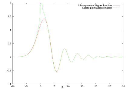
Figure 1: The Wigner function $W_{\mathrm{uq}}$ in the ultraquantum limit, for fixed values of $x$ and $t$.

For small values of $p$, the approximation breaks down as expected, but it becomes quite precise for large values of $|p|$, which encompasses the oscillatory region. Introducing $\kappa=3Qp-\sigma_{p}^{2}/4$, the approximation is different for positive and negative values of $\kappa$. In the first case we have

$$2\sqrt{\pi}\kappa^{-1/4}\cos(2\kappa^{3/2}/(27Q^{2})-\pi/4)\,\exp\{-p\sigma_{p}^{2}/(6Q)+\sigma_{p}^{3}/(108Q^{2})\}$$ (15)

while for negative $\kappa$ we have

$$\sqrt{\pi}|\kappa|^{-1/4}\exp\{-2|\kappa|^{3/2}/(27Q^{2})-p\sigma_{p}^{2}/(6Q)+\sigma_{p}^{3}/(108Q^{2})\}$$ (16)

Notice that for large $p$ the argument of the cosine is proportional to $p^{3/2}/Q^{1/2}$, so that it broadens for large times. Despite the complicated behavior of the Wigner function in this ultraquantum case, all expectation values of $f(x)$ are time independent.

One can go beyond this approximation by considering also the second term on the right-hand side of the Wigner function equation. This approximation is equivalent to the infinite mass limit $m\longrightarrow\infty$. The new Wigner function is obtained from $W_{\mathrm{uq}}(x,p,t)$ by replacing $p$ by $p+V^{\prime}(x)t$. Again, all expectation values of $x$ are time independent.

Many variables

The previous results generalize to more than one variable in a fairly straightforward fashion. The equation satisfied by the Wigner function becomes:

$$\partial_{0}W(\vec{x},\vec{p},t)=-\sum_{n}\left(\frac{p_{n}}{m}\frac{\partial W}{\partial x_{n}}+\frac{\partial V}{\partial x_{n}}\frac{\partial W}{\partial p_{n}}\right)-\frac{\hbar^{2}}{24}\sum_{n,m,r}\frac{\partial^{3}V}{\partial x_{n}\partial x_{m}\partial x_{r}}\,\frac{\partial^{3}W}{\partial p_{n}\partial p_{m}\partial p_{r}}$$ (17)

Now we will consider two particularly important cases. The first one is a O(N) symmetric potential:

$$V=\frac{\mu^{2}}{2}||\vec{x}||^{2}+\frac{\lambda}{8}\left(||\vec{x}||^{2}\right)^{2}$$ (18)

With this potential the last term on the right-hand side of the Wigner function equation becomes

$$\frac{\hbar^{2}\lambda}{8}\sum_{n}\sum_{m}x_{n}\frac{\partial^{3}W}{\partial p_{n}\partial p_{m}^{2}}$$ (19)

An interesting situation occurs when the initial distribution is O(N) invariant. The Wigner function at all times would only depend on invariants ($A=\vec{x}\cdot\vec{p}$, $B=||\vec{p}||^{2}$, and $C=||\vec{x}||^{2}$. The corresponding equation for $W(\vec{x},\vec{p},t)=F(A,B,C,t)$ is given by

$$\partial_{0}F=(-\frac{B}{m}+\mu^{2}C+\frac{\lambda}{2}C^{2})\frac{\partial F}{\partial A}-\frac{2A}{m}\frac{\partial F}{\partial C}+2A(\mu^{2}+\frac{\lambda}{2}C)\frac{\partial F}{\partial B}-$$

$$\hskip 82.51282pt-\frac{\lambda\hbar^{2}}{8}\left(C^{2}\frac{\partial^{3}F}{\partial A^{3}}+6AC\frac{\partial^{3}F}{\partial A^{2}\partial B}+4(2A^{2}+BC)\frac{\partial^{3}F}{\partial B^{2}\partial A}+8AB\frac{\partial^{3}F}{\partial B^{3}}\,+\right.$$

$$\left.+\,(2N+4)C\frac{\partial^{2}F}{\partial A\partial B}+(4N+8)A\frac{\partial^{2}F}{\partial B^{2}}\right)\hskip 48.36958pt$$ (20)

If the initial Wigner function has typical values of $A$, $B$ and $C$ proportional to $N$, as in the case of independent variables, and we scale $\lambda$ to be proportional to $1/N$, the quantum evolution preserves these properties. It is interesting to notice, that in this case the quantum-term in the evolution of the Wigner function is suppressed by one or two powers of $N$ in the denominator. This means that in this particular large $N$ limit, the typical expansion parameters for the quantum evolution is

$$\frac{\hbar^{3}\lambda}{16N\sigma_{p}^{4}}$$

This is consistent with the conventional assertion that the large N dynamics is classical. Furthermore, notice that those terms containing third derivatives are suppressed by two powers of $N$, instead of one. Thus, to leading order in $1/N$ the Wigner function satisfies a simplified equation containing only second derivatives. After some work one can write this leading quantum term as:

$$-\frac{\hbar^{2}N\lambda}{8(BC-A^{2})}\sum_{n,m}x_{m}(Cp_{n}-Ax_{n})\frac{\partial^{2}F}{\partial p_{n}\partial p_{m}}$$ (21)

The second case which we want to consider is that in which the coordinates are labeled by $\vec{n}$, the points of a d-dimensional hypercubic lattice $\Lambda$. The coordinates will be referred as $\phi(\vec{n})$, and the corresponding Hamiltonian is given by

$$H=\sum_{\vec{n}\in\Lambda}\left(\frac{\pi(\vec{n})^{2}}{2m}+\frac{1}{2a^{2}}\sum_{\mu}(\phi(\vec{n}+\vec{\mu})-\phi(\vec{n}))^{2}+\frac{\mu^{2}}{2}\phi^{2}(\vec{n})+\frac{\lambda}{24}\phi^{4}(\vec{n})\right)$$ (22)

The main property of this family of Hamiltonians is its invariance under the symmetry group of translations in d dimensions. Notice that this corresponds to the discretization of the Hamiltonian of a $\lambda\phi^{4}$ scalar field theory in d-dimensions on a lattice of spacing $a$. The quantity $\pi(\vec{n})$ is the conjugate momentum to $\phi(\vec{n})$, satisfying canonical commutation relations among them. If we apply the general formulas to derive the quantum Liouville equation for the Wigner function in this case, we obtain that the quantum term is given by:

$$-\frac{\lambda\hbar^{2}}{24}\sum_{\vec{n}\in\Lambda}\phi(\vec{n})\frac{\partial^{3}W}{\partial\pi(\vec{n})^{3}}$$ (23)

Formally, it is possible to take the continuum limit $a\longrightarrow 0$ and write down the equation satisfied by the Wigner function in the case of quantum field theory. Here we will not be using it so we will not write it down explicitly. The reader can consult Ref. Mrowczynski:1994nf where it is spelled out.

III Langevin approach to quantum evolution

In this section we will try to generate the Wigner function quantum evolution equation by means of a Langevin process. A typical Langevin dynamical process cannot do the job, since it preserves the positive character of the probability density. Hence, we need a non-trivial modification of the standard technique to apply to this case. In what follows we will see how this comes out exactly.

Let us begin by writing the classical evolution equations with the addition of a random force:

$$\dot{x}(t)=\frac{p(t)}{m}\>\>\>\>\>\>\>\>\>\>\>\>\>\>\>\>\>\>\>\>\>\>\>\>\>\>\>$$ (24)

$$\dot{p}(t)=-V^{\prime}(x(t))+F(t)$$ (25)

Our goal will be to study the properties of the force $F(t)$ to recover the equation for the Wigner function. In order to do so in a simplified manner, let us discretize the time variable and write the equation relating $x^{\prime}\equiv x(t+\delta t)$ and $p^{\prime}\equiv p(t\ +\delta t)$ to $x\equiv x(t)$ and $p\equiv p(t)$:

$$x^{\prime}=x+\delta x=x+\delta t\,\frac{p}{m}\,\>\>\>\>\>\>\>\>\>\>\>\>\>\>\>\>\>\>\>\>\>\>$$ (26)

$$p^{\prime}=p+\delta p=p-V^{\prime}(x^{\prime})\,\delta t+\delta F(t)$$ (27)

As we will see, to spell out the $x$ dependence of the random force, we should write $\delta F(t)=x^{1/3}(t)\eta(t)$, where the distribution of the variable $\eta(t)$ is controlled by a function $\rho(\eta)$. Now, let us write the distribution function for $x^{\prime}$ and $p^{\prime}$, which by definition is $W(x^{\prime},p^{\prime};t+\delta t)$. We get

$$W(x^{\prime},p^{\prime};t+\delta t)=\int d\eta\>\int dx\,dp\ \rho(\eta)\,W(x,p,t)\,\delta(x^{\prime}-x-\delta x)\,\delta(p^{\prime}-p-\delta p)$$ (28)

Now we should eliminate the integrals over $x$ and $p$ with the use of the delta functions. For that purpose we should make use of the time-reversed evolution equations

$$x=x^{\prime}-\delta t\,\frac{p}{m}\equiv f(x^{\prime},p^{\prime},\eta)\>\>\>\>\>\>\>\>\>\>\>\>\>\>\>\>\>\>\>\>\>$$ (29)

$$p=p^{\prime}+V^{\prime}(x^{\prime})\,\delta t-x^{1/3}\eta\equiv g(x^{\prime},p^{\prime},\eta)$$ (30)

We get

$$W(x^{\prime},p^{\prime},t+\delta t)=\int d\eta\,\rho(\eta)\ W(f(x^{\prime},p^{\prime},\eta),g(x^{\prime},p^{\prime},\eta),t)\ J(x^{\prime},p^{\prime})$$ (31)

where $J$ is the jacobian of the change of variables. Finally, we expand the equation in powers of $\delta t$ and $\eta$. Keeping terms linear in $\delta t$ only, we obtain a discretized version of the quantum Liouville equation provided we demand

$$\int d\eta\,\rho(\eta)=1\>\>\>\>\>\>\>\>\>\>\>\>\>\>\>\>\>\>\>\>\>\>\>\>\>\>\>\>\>\>\>\>\>\>\>\>\>\>\>\>\>\>\>\>\>\>\>\>\>\>$$

$$\langle\eta^{n}\rangle\equiv\int d\eta\,\rho(\eta)\ \eta^{n}=0\quad\mathrm{for}\ 0<n\neq 3$$ (32)

and

$$\langle\eta^{3}\rangle\equiv\int d\eta\,\rho(\eta)\ \eta^{3}=\frac{\lambda\hbar^{2}\,\delta t}{4}$$ (33)

It is quite obvious that if the variable $\eta$ is real, the previous equations are incompatible with a positive definite distribution function $\rho(\eta)$, since in that case $\langle\eta^{2n}\rangle\geq 0$ or all moments should be 0. Despite this fact in the next section we will see how we can relate the equation to that of a truly positive-definite distribution function, for which sampling statistical methods are applicable.

The generalization of the previous formulas to the case of several variables is fairly straightforward. In principle, the force is now replaced by a vector of forces $\delta F_{i}$. These forces are functions of several random variables with non-positive definite distribution functions. A simple way to parametrize these forces is

$$\delta F_{i}=\eta\chi_{i}$$ (34)

where the distribution function of $\rho(\eta)$ coincides with the one of a single variable. The remaining variables $\chi_{i}$ can be distributed according to standard positive-definite distributions.

As an example consider the case of the O(N) symmetric potential. In this case one can write $\chi_{i}=x_{i}\tau+\xi_{i}$ and choose a simple positive definite distribution function $\tilde{\rho}(\tau,||\vec{\xi}||)$ to recover the time-discretized version of the Wigner-function equation. We leave the details to the reader.

For the case of a d-dimensional lattice field potential given in the previous section, a choice like $\chi_{i}=x^{1/3}_{i}\xi_{i}$ will do, provided the $\xi_{i}$ are independent random variables with vanishing average and $\langle\xi^{3}_{i}\rangle=1$.

IV A new computational method

In the previous section we have seen how to reproduce the evolution equation for the Wigner function by means of a Langevin approach with a random force with non-positive definite distribution function. This is the starting point for a new procedure to approximate the quantum evolution which we will explain in this section. The method depends on three steps or approximations which are intimately connected among themselves. The first part is a coarse-grain approximation in the momenta $p_{i}$, with a characteristic coarse-graining parameter $\epsilon$. Next we will show how one can reproduce the effect of the non-positive definite distribution function $\rho(\eta)$ by means of a purely Markovian process involving ordinary probability measures. This will allow the use of standard sampling techniques to generate the distribution. The last step will be the introduction of a parameter $\kappa$ multiplying the quantum term in the evolution equation for the Wigner function. The parameter interpolates between a purely classical evolution ($\kappa=0$) and the full quantum evolution (for $\kappa=1$). The whole procedure can be used to compute the evolution of quantum expectation values in powers of $\kappa$. This is similar to an expansion in powers of $\hbar^{2}$, although part of the $\hbar$ dependence sits in the initial condition and is left unchanged.

As mentioned in the previous paragraph, our first step is a coarse-grain approximation, which will amount to an approximation to the non-positive definite $\rho(\eta)$. For that purpose, we might relax the condition that $\langle\eta^{n}\rangle=0$ for $n>3$. One possible realization of the conditions is achieved by the following family of distribution functions:

$$\rho_{N}(\eta)=\delta(\eta)+\sum_{i=1}^{M_{N}}\frac{\gamma_{i}}{\epsilon^{3}}(\delta(\eta-\epsilon\alpha_{i})-\delta(\eta+\epsilon\alpha_{i}))$$ (35)

where $\gamma_{i}$ are positive numbers, $\alpha_{i}$ are real values, and $\epsilon$ is a free parameter. Although not explicitly indicated, the coefficients $\gamma_{i}$ and $\alpha_{i}$ do depend on N. They are determined by imposing that all even moments vanish and odd moments, given by

$$\mu_{2p+1}\equiv\langle\eta^{2p+1}\rangle_{N}=2\sum_{i=1}^{M_{N}}\gamma_{i}\,\alpha_{i}^{2p+1}\epsilon^{2(p-1)}$$ (36)

vanish for $p\leq N$, with the exception of $p=1$ given by Eq. 33. If we take, without loss of generality, that the parameters $\alpha_{i}$ are of order 1, this condition implies that

$$\gamma_{i}\propto\frac{\lambda\,\hbar^{2}\,\delta t}{8}$$ (37)

In general, the solution to the set of constraints will not determine the parameters $\gamma_{i}$ and $\alpha_{i}$ uniquely. This freedom in the choice of the parameters is a bonus, since one can test the effects of the coarse-graining on the results, by exploring different choices. Furthermore, a better approximation is obtained by taking larger values of $N$, which will be referred as the level of the approximation. The number of terms $M_{N}$ has to grow as $N$ grows. An alternative method to improve the accuracy would be to reduce the value of $\epsilon$, thus reducing the effect of higher order derivatives of the Wigner function. As we will see later, there is a limitation to the minimal value of $\epsilon$, which is dictated by the range of time for which the method would be applicable.

The next ingredient will be that of relating the Wigner function to a positive-definite distribution function, which can be approximated by samples. The same can be done for the distribution function $\rho(\eta)$ as follows. Let us introduce a positive-definite function $\hat{\rho}(\eta,\sigma)$ involving a discrete Ising-like variable $\sigma=\pm 1$. This function is related to $\rho(\eta)$ by

$$\rho(\eta)=\mathcal{N}\sum_{\sigma=\pm 1}\hat{\rho}(\eta,\sigma)\,\sigma$$ (38)

The function $\hat{\rho}(\eta,\sigma)$ is normalized as a probability distribution

$$\sum_{\sigma}\int d\eta\,\hat{\rho}(\eta,\sigma)=1$$ (39)

and hence the prefactor is given by:

$$\frac{1}{\cal N}=<\sigma>_{\hat{\rho}}\,\equiv\sum_{\sigma}\int d\eta\,\hat{\rho}(\eta,\sigma)\,\sigma$$ (40)

The construction can be extended to the coarse-grained version given before. Hence, we define

$$\hat{\rho}_{N}(\eta,\sigma)=\frac{1}{\cal N}\left[\frac{1+\sigma}{2}\,\delta(\eta)+\sum_{i=1}^{M_{N}}\frac{\gamma_{i}}{\epsilon^{3}}\,\delta(\eta-\epsilon\alpha_{i}\sigma)\right]$$ (41)

The normalization condition implies

$${\cal N}=1+2\sum_{i=1}^{M_{N}}\frac{\gamma_{i}}{\epsilon^{3}}$$ (42)

A similar procedure can be applied to the Wigner function

$$W(x,p;t)=K(t)\sum_{\sigma=\pm 1}\hat{W}(x,p,\sigma;t)\,\sigma$$ (43)

where $\hat{W}(x,p,\sigma;t)$ is a well-defined probability distribution. This is equivalent to writing the Wigner function as the difference of two positive definite functions. If we label by $\langle\ \rangle_{\hat{W}}$ the expectation values with respect to $\hat{W}(x,p,\sigma;t)$, then the expectation values with respect to the Wigner function are given by

$$\int dx\,dp\ O(x,p)\,W(x,p;t)=\frac{\langle\sigma\,O(x,p)\rangle_{\hat{W}}}{\langle\sigma\rangle_{\hat{W}}}$$ (44)

Now, one can obtain a time-discretized evolution equation for $\hat{W}(x,p,\sigma;t)$ involving $\hat{\rho}(\eta,\sigma)$ as follows:

$$\hat{W}(x,p,\sigma;t+\delta t)=\sum_{\mu=\pm 1}\int d\eta\,\hat{\rho}(\eta,\mu)\hat{W}(x-\delta x,p-\delta p,\mu\cdot\sigma;t)$$ (45)

where the displacements $\delta x$-$\delta p$ are those coming from the classical equations of motion with a force proportional $\eta$ (as before). Summing the previous equation over $\sigma$ and using the previous definitions, we re-obtain the discretized evolution equation for the Wigner function provided

$$K(t+\delta t)={\cal N}K(t)$$ (46)

We see that this implies that the normalization factor grows exponentially, and this is precisely the main numerical limitation of the method.

Having set up an evolution equation for the probability distribution $\hat{W}(x,p,\sigma;t)$ we can employ standard sampling techniques to approximate it. This leads us to the concept of signed samples: a collection of ${\cal M}$ points $\{x^{(a)},p^{(a)},\sigma^{(a)}\}$ such that

$$\int dx\,dp\,\sum_{\sigma=\pm 1}\hat{W}(x,p,\sigma;t)\,O(x,p;\sigma)\approx\frac{1}{\cal M}\sum_{a=1}^{\cal M}O(x^{(a)},p^{(a)};\sigma^{(a)})$$ (47)

From Eq. 45 one can determine the time evolution of samples given a realization of the noise $\eta$. This is a Markovian process where $\hat{\rho}(\eta,\mu)$ determines the conditional probability for a transition from one point in phase-space to a new one and a possible change of sign of the discrete Ising variable.

If we use the coarse-grained distribution $\hat{\rho}_{N}(\eta,\mu)$, then with a certain probability we would simply evolve the system with the classical equations of motion, and with probability proportional to $\delta t$ we would produce a jump in the value of momentum and a possible flip of the sign of $\sigma$. The reason for referring to the first approximation as coarse-graining in momentum space, has to do with the discrete magnitude of the jump (of order $\epsilon$) at each step of the time-evolution. If the Wigner function would be a polynomial in $p$, the approximation would be exact.

If we start the evolution with a positive definite Wigner function, then $\frac{1+\sigma}{2}W(x,p,t=0)=\hat{W}(x,p,\sigma,t=0)$. Hence, all points in the sample have $\sigma^{(a)}=1$. As time evolves some of the points acquire a negative value of $\sigma^{(a)}$. At time $t=n\delta t$ the probability that a point in the sample has negative $\sigma$ is given by

$$P_{-}=\frac{1-\langle\sigma\rangle_{\hat{W}}}{2}=\frac{1}{2}\,(1-(<\sigma>_{\hat{\rho}})^{n})\approx\frac{1}{2}\,(1-e^{-At\lambda\hbar^{2}/\epsilon^{3}})$$ (48)

with $A$ a number of order 1, which depends on the detailed form of $\hat{\rho}_{N}$. The probability approaches $1/2$ exponentially in time. Once this happens we encounter a severe sign problem in computing averages according to the formula Eq. 44, since the averages result from strong cancellations from $\sigma=1$ and $\sigma=-1$. At this point the method breaks down. The typical time when this happens is given by

$$T\approx\frac{\epsilon^{3}}{\lambda\hbar^{2}}$$ (49)

Clearly things get worse as we decrease $\epsilon$ and improve as we decrease $\lambda$ and $\hbar$. However, the magnitude of $\epsilon$ must be related to the typical range of variation in $p$ of the Wigner function. Otherwise, corrections involving higher order derivatives of the Wigner function become large. The systematic errors associated to the coarse-graining can be checked by varying $\epsilon$ or by using different choices of $N$. For small enough $\epsilon$, the approximation should behave better for larger $N$.

Once the maximum acceptable value of $\epsilon$ is selected, the method stated before only allows the computation of quantum expectation values for a range of times. This limitation, although important, does not destroy the usefulness of the method. Time-range limitations are already present in studying the classical evolution equation of a quantum field theory discretized on a lattice. The moment that the fluctuations become sizable at the cut-off scale, the discretized evolution equation fail to reproduce the continuum evolution. Fortunately, in many applications a good part of the interesting physical processes take place in a relatively short period of time. This is the case, for example, in the context of preheating in the early universe, which is one of the main motivations that we had for embarking in the present work.

In situations in which a reliable full quantum evolution can only be carried for a too short lapse of time, the method can be used to compute first-order quantum corrections as follows. This is the third ingredient that we anticipated in the first paragraph of this section. The strategy is to consider a modified evolution equation with a new parameter $\kappa$ multiplying the last term of Eq. 10. This can be interpreted as multiplying $\hbar$ by $\sqrt{\kappa}$. In this fashion one extends the time range of applicability of our method by the multiplicative factor $1/\kappa$. Now, evolving the system for several other smaller values of $\kappa$, one can determine the evolution of the expectation values as a power series in $\kappa$.

A practical problem concerns accuracy. Since, our goal is to estimate the quantum fluctuations, we realize that when reducing $\kappa$, they have decreased by the same factor. To maintain the signal to noise ratio one should increase the size of the sample by $\kappa^{2}$, which would increase the computation time by the same factor. Since the reduction in $\kappa$ was dictated by the necessity to extend the range in time of the simulation, we conclude that this can be done at a cost in computer time which only grows polynomially with this range.

Of course, the drawback is that one does not compute the full quantum effects but only to leading order in $\kappa$ (i.e. $\hbar^{2}$). This by itself is an important result because it would serve as a measure of the size of quantum effects and as a next-to-leading correction to the classical approximation. Higher order powers of $\kappa$ are also computable at a higher cost in computer time.

To test these ideas we decided to study several simple quantum mechanical systems for which the exact quantum evolution can be determined by numerical integration of the Schroedinger equation. The results will be presented in the next section and compared to other extensions of the classical approximation given in the literature.

Before closing this section, we should comment on the modifications necessary to extend the procedure defined previously to the case of many degrees of freedom. Our method might not be optimal for the case of very few degrees of freedom, however, it was designed to be extensible in an affordable way to the case of many degrees of freedom. In this respect it differs from other proposals in the literature based on histogramming which seem impossible to extend to a large number of variables.

The formal extension of all the approximations involved in the method to the case of several degrees of freedom is indeed trivial. In the way that the Langevin process was extended at the end of the last section, it turns out that there is a unique random variable $\eta$ having a non positive definite distribution function with similar or exact properties as the one appearing for the one-variable case. Thus, the coarse graining $\rho\longrightarrow\rho_{N}$ and extension to positivity $\rho(\eta)\longrightarrow\hat{\rho}(\eta,\sigma)$ remains exactly the same irrespective of the number of variables. The rest of random variables entering the force are of the conventional type and their number increases linearly with the number of degrees of freedom, and so does the computation time for a given time-step. The sample now, however, involves trajectories in the multidimensional state of the system. This is exactly the same as for the classical evolution (with random initial conditions), except that now there is a single additional Ising-like variable $\sigma$. Thus, for a fixed number of trajectories the computational cost will grow in a similar fashion to that of the classical evolution. A new question to worry about is whether the number of trajectories needed to obtain results with a reasonable accuracy depend upon the number of degrees of freedom. This will be studied in the next chapter for one particular example.

V Testing the classical approximation and its extensions

In this section we will present the results of our tests of the classical approximation and of our proposed method to obtain quantum corrections, together with other proposals. The first cases are particularly simple situations with one or two degrees of freedom for which the exact quantum evolution can be obtained through the numerical integration of the Schroedinger equation. Later we will explore the first steps towards a possible application to quantum field theory.

Our first example will be a simple anharmonic oscillator at intermediate values of the self-coupling. The potential is that given in Eq. 8 with the following choice of parameters:

$$m=1\quad;\quad\quad\mu^{2}=0.5\quad;\quad\quad\lambda=0.45$$ (50)

The value of the dimensionless parameters mentioned in Section 2 are given by $r=s=1.57$. We choose as initial condition a gaussian pure state with width given by $\sigma\mu^{2/3}=0.45/2^{1/3}$. Our main observable was taken to be the expectation value of the square of the position operator $Q^{2}$ as a function of time, which is noted $\langle Q^{2}\rangle(t)$. The Hamiltonian, the initial state and the observable were used in a previous paper with a similar spirit to ours Aarts:2006cv . However, for illustrative purposes we are presenting the results for a higher value of the self-coupling $\lambda$, for which quantum effects are stronger.

The main results are collected in Fig. 2-2. In the first figure the time evolution of the observable is displayed in units of the half-period of the $\lambda=0$ system. This expectation value performs oscillations with a frequency close to that of the $\lambda=0$ system. The classical approximation, also displayed in the figure, oscillates as well, but the amplitude gets damped very fast with time. This damping is a typical feature of the classical approximation which has been pointed out repeatedly (including Ref. Aarts:2006cv ).

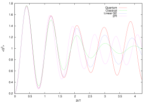
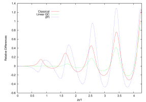
Figure 2: (a): Time evolution of $\langle Q^{2}\rangle$ compared to the classical approximation, the 2PI truncation to NLO order in 1/N expansion, and the method proposed in this paper. (b): Relative error committed in each of the approximations as a function of time.

The figure also shows two other curves. The first being the 2PI approximation obtained by keeping only the leading and next-to-leading (NLO) diagrams in a 1/N expansion Berges:2001fi . Notice that in this case the amplitude of the oscillation is not decreasing, but there is a shift in the period oscillation. This might not be a serious drawback in extracting average properties over time. Finally, we also present the result of the new method explained before, which includes the classical approximation and the leading $\hbar^{2}$ correction. The exact details are explained below.

In Fig. 2 we present relative error of each approximation, namely the difference between the quantum evolution and the corresponding approximation, divided by the quantum result. The first line corresponds to the classical approximation, which oscillates with increasing amplitude. Quantum corrections start being negligible and grow to a 20% level at $2t/T\approx 0.8$, and 40% level at $2t/T\approx 2.5$. The 2PI curve appears to be the worst, but this is due to the shift in period with respect to the quantum curve. A more fair presentation should involve a comparison of the height of the maxima, for which 2PI is certainly better than the classical approximation. The last curve is our calculation including quantum effects up to linear order in $\hbar^{2}$, using the method described in the previous section. Notice, that it provides a very accurate description of the quantum effects up to $2t/T\approx 1.4$. Beyond this point it has more sizable errors, but certainly smaller than the classical approximation. Furthermore, it provides at least an estimate of the errors committed by employing the classical approximation.

The actual procedure that we followed to determine the leading quantum correction (LQC) is the following. We re-scaled the size of the quantum term of quantum Liouville equation by using $\kappa$. Then, we used the coarse-grained approximation to $\rho(\eta)$ up to the second level ($N=2$, $\langle\eta^{5}\rangle=0$ but $\langle\eta^{7}\rangle\neq 0$), and the sampling method described in the previous chapter, to study the quantum evolution equation for a given value of $\kappa$. The formula to obtain the approximation (LQC) including the contribution linear in $\hbar^{2}$ to any observable $O$ is

$$O_{\mathrm{LQC}}=O_{\mathrm{clas}}+\frac{1}{\kappa}(O_{\kappa}-O_{\mathrm{clas}})$$ (51)

The curves depicted in Fig. 2 were obtained using $\kappa=1/6$.

To check whether $\kappa=1/6$ is in the linear regime, and to give an estimate of the size of the higher order terms in $\hbar^{2}$, we repeated the procedure and obtained $O_{\kappa}$ for several values of $\kappa$ ($\kappa=0,1/10,1/8,1/6,1/5,1/4,1/2$). In this way we get an idea about how the value of the observable interpolates between the classical ($\kappa=0$) and the quantum value ($\kappa=1$). In Fig 3 we display the result obtained for the expectation value of $Q^{2}$ at the position of the third maximum ($2t/T=2.1$). The y-axis gives the values obtained for the different values of $\kappa$ mentioned previously. We also display the value for the classical approximation ($\kappa=0$) and the full quantum result ($\kappa=1$). It is quite clear that the results follow an approximate linear dependence for $\kappa<1/3$. The straight line is the result of a linear fit (1 free parameter) in this range. The extrapolation to $\kappa=1$ of the straight line is very approximately our estimate of the quantum evolution up to next-to-leading order in $\hbar^{2}$ (the leading order being the classical approximation). In this particular case we see that the linear quantum correction term (LQC) accounts for 80% of the quantum effects. Thus, with the addition of the classical approximation, we reproduce the exact quantum result with a 3% error. In principle, one could go beyond the linear approximation and determine higher order corrections in $\hbar^{2}$. If we add the result of $\kappa=0.5$ to the data and fit the results to a second degree polynomial in $\hbar^{2}$ we get an even better approximation to the quantum result (second line in Fig. 3).

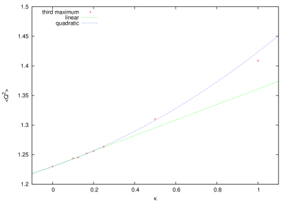
Figure 3: The value or $\langle Q^{2}\rangle$ at the third maximum in time computed using several values of $\kappa$ (see text). The lines are linear and quadratic fits.

Although the previous results by themselves show that our procedure cannot be completely misguided, we have analyzed the different sources of error in the determination of the $\hbar^{2}$ correction presented above. Using jack-knife methods we can quantify the purely statistical errors. They increase with time but remain always at the level of a few percent. A much more difficult estimate is the effect of the coarse-graining in momenta. This can be estimated by changing the value of $\epsilon$ and/or adding more terms in the discretization to impose $\langle\eta^{2M+1}\rangle=0$. In particular, we have used results at $\epsilon=0.3$ and three levels of discretization. The effect is more pronounced at the maxima and minima of the oscillations and the better the approximation, the closer the results to the actual quantum evolution. We estimate that, at most, errors (to the quantum correction) could be of the order of 10-15% at the third maximum ($2t/T=2.1$) rising up to 20-25% at the fourth maximum ($2t/T=3.0$). The same conclusion follows both by comparison of the different levels as well as by extrapolation in $\epsilon^{\alpha}$ (with $\alpha\approx 3$) to $\epsilon=0$. The conclusion is that, even if the errors are sizable, the method provides a good estimate of the quantum effects.

Before embarking into the generalization to several variables, we tested the situation for another case having several distinct features which are present in some of the phenomenological applications to cosmology. We considered a potential of the form

$$V(x,t)=-\frac{1}{2}\mu^{2}\tanh(\alpha t)x^{2}+\frac{\lambda}{4!}x^{4}$$ (52)

with the parameters chosen to be

$$\mu^{2}=2\quad;\quad\quad\alpha=0.2\quad;\quad\quad\lambda=0.4$$ (53)

This time-dependent potential provides a smooth interpolation between a single-well and a double-well potential mimicking the situation occurring in hybrid inflationary models. Notice that tunneling effects are possible now. The initial condition is a pure state given by a gaussian with $\sigma\mu^{2/3}=1/4^{1/3}$. The same observable as before, $\langle Q^{2}\rangle$, is displayed in Fig. 4 for a range of times for which the potential has basically evolved to the future asymptotic potential. Hence, as expected, the expectation value migrates from its initial value to performing oscillations around $x_{min}^{2}$, where $x_{min}$ is the minimum of future asymptotic potential. Also shown, is the corresponding curve for the same 2PI approximation mentioned earlier. Although following the pattern of the quantum result, the differences are substantial. On the other, hand the classical evolution works quite well for this case. However, the addition of the Linear Quantum correction (LQC) using our method (with $\kappa=1/2$) makes the result much better, as can be seen when looking at Fig. 4, where we display the relative differences with respect to the quantum evolution as before.

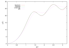
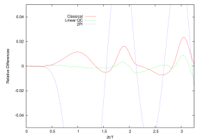
Figure 4: (a): The same as Fig. 2 but for the potential in Eq. 52. (b): Relative differences as in Fig. 2.

A full comparison of competitive methods suggested us to include the results of the Complex Langevin method described in Berges:2005yt , and we invested considerable effort in doing so. The method generates a collection of histories as a function of an additional time variable. Our naive implementation, however, led to a growing number of trajectories blowing up in this additional time. It is easy to see that this is a feature of the complex evolution in the discretized new variable and in the absence of random noise. Both the problem and the possible cures have been documented in the literature of the subject. One can employ more refined discretizations or use a much smaller Langevin step Berges:2005yt , but this pays an obvious price in computational cost. A way out proposed in Ref. Aarts:2009dg is to use an adaptive stepsize. Another possibility is a modification of the noise Aarts:2009uq . Using these techniques we were able to eliminate most of the divergent trajectories. A small fraction, but growing in extra-time, remained. We took the attitude mentioned in Ref. Berges:2005yt to discard them or go back in time and re-evolve them.

Another problem mentioned in the literature is the issue of convergence. Sometimes the system can show a limited decay to the equilibrium distribution or can converge to a wrong limit Aarts:2009uq Aarts:2011ax . This seems to be case in our tests of the previous examples. Furthermore, the results obtained seemed robust under changes of the methodology (adaptive step, different stepsizes, discarding or re-evolving) and stable under further evolution in the additional time. These results did not even show the right oscillatory pattern already seen in the classical approximation. Some authors Aarts:2011ax claim that to ensure the correct convergence other modifications are necessary. However, given that this was not the main issue of this paper, we decided to drop out these results and defer its study to further scrutiny.

Extension to several variables

Since our ultimate goal is that of studying the quantum evolution of fields, it is crucial to determine how does the new method that we have presented depend upon the number of degrees of freedom. The standard non-perturbative treatment of quantum fields proceeds through a lattice discretization and a subsequent continuum limit. Renormalization is a crucial ingredient in the process to obtain meaningful physical results. The latter aspect lies somewhat far from the scope of this paper and will be addressed in a future publication. The focus here is rather upon the numerical feasibility of the procedure. For attaining acceptable results one has to reach a number of variables within the range of those customary for these kind of simulations. A priori, the method presented here is capable of doing so, since its computational effort is comparable to that involved in the classical approximation for a given number of sampling trajectories, which has been used successfully in this context.

However, there is a point of concern which we want to address. It might well happen that the number of trajectories needed to attain a given precision in the estimation of the quantum corrections grows with the number of degrees of freedom: A polynomial growth is acceptable, an exponential growth is not.

As a testing example we have considered a lattice version of a two-dimensional scalar field theory which has been studied by other authors in this same context Salle:2001xv . We take a real scalar quantum field in $1+1$ dimensions with Hamiltonian

$$H(t)=\int dx\Big{[}\frac{1}{2}\pi^{2}(x,t)+\frac{1}{2}(\nabla\phi(x,t))^{2}+\frac{1}{2}\mu^{2}\phi^{2}(x,t)+\frac{\lambda}{24}\phi^{4}(x,t)\Big{]}$$ (54)

where $\mu^{2}$ may depend on t. We have already explained the influence of $\hbar$ factors, so from now on we assume natural units, $\hbar=c=1$. The dimensionless field $\phi$ and its conjugate momentum $\pi=\dot{\phi}$ satisfy equal-time canonical commutation relations

$$[\pi(x),\phi(y)]=-i\,\delta(x-y)$$ (55)

which gives $\pi(x)$ dimensions of inverse length.

The next step is to consider the lattice version of the previous Hamiltonian. Continuous space is approximated by a discrete number of points $x_{n}=na$ separated by a distance $a$, the lattice spacing. To deal with a finite number of variables we must, in addition, put the system in a box of size $L$ with periodic boundary conditions. Altogether, we end up having $N=L/a$ variables $\phi_{n}(t)\equiv\phi(na,t)$. The corresponding conjugate momenta $\pi_{n}(t)$ satisfy the commutation relations

$$[\pi_{n},\phi_{m}]=-\frac{i}{a}\,\delta_{nm}$$ (56)

where the factor of $a$ is necessary to preserve the dimensions of the conjugate momentum. Naive discretization then leads to the Hamiltonian

$$H=\sum_{n=0}^{N-1}a\Big{[}\frac{1}{2}\pi_{n}^{2}+\frac{1}{2}(\nabla\phi_{n})^{2}+\frac{1}{2}\mu^{2}\phi_{n}^{2}+\frac{\lambda}{24}\phi_{n}^{4}\Big{]}$$ (57)

with $\nabla\phi_{n}=(\phi_{n+1}-\phi_{n})/a$. After a suitable rescaling of the variables and of the parameters the Hamiltonian can be cast in the form Eq. 22.

After presenting our system and its discretized version, let us consider the dynamical process that we will study following Ref. Salle:2001xv . The idea is to study the evolution of the system after a quench. In practice, this means that the $\mu^{2}$ parameter flips its sign abruptly at time $t=0$ from a positive value to a negative one. This can be seen as a limiting version of our previously smooth ($\tanh$) transition from single to double-well.

In practice, what we will consider is the evolution of the system for positive times starting (at $t=0$) from an initial state given by the ground state of the Hamiltonian with $\lambda=0$ and positive $\mu^{2}$. This initial state is therefore gaussian as in previous examples, and is easily generated. For our numerical simulation we have taken the parameters of the model to be

$$\lambda=3m^{2}\quad\quad a=0.8/m$$ (58)

where the unit of mass $m$ is given by $m=\sqrt{-2\mu^{2}}$. Then we have studied this model for $N=2$,$4$,$8$,$16$ and $32$.

For a real quantum field theory application one has to study the limit of $a$ going to $0$, with a suitable tuning of the parameters dictated by the renormalization conditions. For very small lattice spacings one might even encounter problems of critical slowing down, but these will affect other methods too. Here, we will be content with scaling the number of degrees of freedom and focusing on statistical significance and computational load alone.

Finally, let us select our observables and present our results. Rather than working with the field variables we can work with their Fourier modes $\hat{\phi}_{k}(t)$, since they decouple in the $\lambda=0$ limit. We use the following normalization for the discrete Fourier transform

$$\hat{\phi}_{k}(t)=\frac{\sqrt{L}}{N}\,\sum_{n=0}^{N-1}e^{-i\frac{2\pi}{N}nj}\,\phi_{n}$$ (59)

where $k=(2\pi/L)j$ for $j=-N/2+1,-N/2+2,{\ldots}.,N/2$. A similar expression applies for the modes $\hat{\pi}_{k}(t)$. Reality of our original field implies $\hat{\phi}_{k}^{*}(t)=\hat{\phi}_{-k}(t)$ (and the same for $\pi$).

As mentioned previously for $\lambda=0$ and positive $\mu^{2}$ all the modes oscillate with a characteristic frequency $\omega(k)=\sqrt{4\sin^{2}(j\pi/N)/a^{2}+\mu^{2}}$. At the classical level, the flip in sign of $\mu^{2}$ produces that the low lying modes acquire an imaginary $\omega(k)$, and start growing exponentially. In the presence of a non-zero $\lambda$ the growth ceases once the non-linear effects become important.

In Fig. 5 we present our results for the sum of expectation values of the square of each mode $\langle\sum_{k}|\hat{\phi}_{k}|^{2}(mt)\rangle$ for two degrees of freedom $N=2$. As a matter of fact this observable is just a discretized version of $\int dx\,\phi^{2}(x)$. The time evolution as a function of $mt$ is given, as obtained from the numerical integration of the $N=2$ Schroedinger equation. The result of the classical approximation and of our LQC method obtained from $\kappa=1/3$ are also shown. The exact numerical integration has negligible errors at the scale of this and the following figures. The errors of the remaining approximations were obtained by applying a jack-knife method to the sample of trajectories. The total number of trajectories used for this data was $\mathcal{M}=8\times 10^{6}$.

The results show the same pattern as before. The classical approximation captures the main features, but our LQC approximation calculation is capable of reducing the discrepancy substantially. Only at the latest times this difference exceeds the level of the statistical errors.

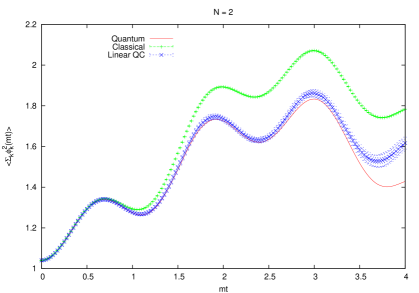
Figure 5: Time evolution of $\langle\sum_{k}|\phi_{k}|^{2}(mt)\rangle$ for $N=2$, for the fully quantum, classical approximation and LQC method for $\kappa=1/3$.

In Fig. 6 and Fig. 6 we display the corresponding results for $N=8$ and $N=32$ with a sample of size $\mathcal{M}=4\times 10^{7}$. Here we do not have an exact result to compare with, so the main issue is the dependence of the errors on $N$ for a fixed sample size. Errors of our method are larger than those of the classical approximation as expected, but do not seem to depend crucially on the number of variables.

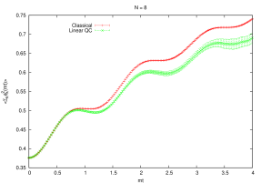
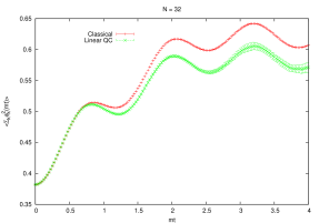
Figure 6: The same as Fig. 5 but for $N=8$ (a) and $N=32$ (b).

The intermediate values of $N$, not shown, display exactly the same pattern. For all values of $N$ the relative difference between classical and linear QC approximation approaches a constant with errors diminishing as the sample size $\mathcal{M}$ grows. For the maximum values studied of order $\mathcal{M}=5\times 10^{7}$, we can estimate the quantum correction at our latest times $mt\approx 3$ with an accuracy of 10% without a significant dependence on the number of degrees of freedom.

In conclusion, the proposed method seems to scale reasonably well with the number of degrees of freedom. The computational cost is only a certain factor higher than that involved in the classical approximation. Thus, phenomenologically interesting applications are addressable within present high performance computing capabilities.

VI Conclusions and Outlook

In this paper we have analyzed the real-time evolution of simple quantum systems. Both the form of the potential, as well as the type of initial conditions are chosen to reflect relevant applications in Cosmology. The simplicity of the systems allows the numerical integration of the Schroedinger equation and, hence, can be used to test different approximation methods. The simplest one is given by the classical approximation which amounts to the classical evolution of a random variable distributed according to the initial wave-function. In our examples the classical approximation always performed well at initial times, capturing the qualitative features of the quantum evolution. When trying to improve on this approximation it seems natural to focus on the Wigner function and the quantum Liouville evolution equation that it satisfies. It is simple to introduce a parameter $\kappa$ in the evolution equation that interpolates between the classical approximation ($\kappa=0$) and the full-quantum evolution ($\kappa=1$). This parameter amounts to a rescaling in the value of $\hbar^{2}$ appearing explicitly in the equation.

We have presented a method based on samples and a discretization (coarse-graining) in the distribution in the conjugate momentum, and compared its results with the classical approximation, the next-to-leading 1/N truncation of the 2PI equations, and the numerical quantum evolution. The method can be used to determine the quantum corrections to the time-evolution of expectation values as a power series expansion in $\kappa$. This provides a natural extension of the classical approximation (corresponding to the lowest-order). The results, for the examples considered, seem to capture a sizable part of the quantum effects, therefore providing a possible alternative to other approaches. Even when the method sizably departed from the exact quantum result, the discrepancy remained smaller and of the order of the quantum effect, and no anomalous instabilities were observed. Thus, it can at least serve to attach a level of precision to the classical approximation.

The method is certainly not a panacea. We emphasize that quantum averages are subject to the sign problem since the Wigner function is not positive definite. Our sampling method is equivalent to reweighting, which is certainly not a solution to the sign problem. However, if one starts with a positive definite distribution function, the problem only sets in at a later time, and reliable estimates of the quantum effects can be obtained at early stages of the evolution. The method can also be used to compute the full quantum effect by setting $\kappa=1$. However at fixed $\kappa$, our coarse-grained sampling method severely breaks down beyond a critical range of times. However, one can go well beyond this point if one aims at computing the quantum corrections to order $\kappa^{n}$ and not the full quantum evolution. In this case, the computational cost only grows in a power-like fashion with respect to the time range of the analysis. This can then be viewed as a systematic improvement with respect to the classical approximation, which at the least can serve to quantify the size of the quantum corrections involved. All other errors, arising from the statistical size of the sample or from the discretization in conjugate momenta are quantifiable.

As emphasized in the introduction, our main goal is to be able to apply the method to the evolution of quantum fields in the early universe. For that purpose it is important to see how the computational cost depends on the number of degrees of freedom. Methods based on histogramming the Wigner function have costs that grow exponentially with the number of variables. In designing the methodology we focused on an approach which only grows in a power-like fashion, even if there are more efficient ways to handle systems with a few degrees of freedom. In the last section we have presented a pilot study to measure the rate at which the computational cost evolves with the number of variables. The comparison is done by monitoring the size of the sample in order to keep the degree of accuracy of the quantum corrections fixed. In our exploratory study we focused upon a two-dimensional quantum field theory case which has been subject of previous study as a toy model for cosmological applications. The model has been discretized to a system with $N$ degrees of freedom. We applied our technique to the model up to $N=32$, and we found that the statistical errors on the quantum effects of our observables for a fixed sample size remain stable with the number of degrees of freedom. Of course, the simulation time grows with the number of degrees of freedom, as does for the case of the classical approximation. Even if computationally demanding, these calculations are feasible with present day technology, and so will be the case for our proposed method. The results presented in this paper allow us to be optimistic enough to embark in a higher scale study with all the complexities involved in a quantum field theoretical treatment.

- (1) P. de Forcrand, PoS LAT2009, 010 (2009), arXiv:1005.0539 [hep-lat]
- (2) J. S. Schwinger, J. Math. Phys. 2, 407 (1961)
- (3) L. V. Keldysh, Zh. Eksp. Teor. Fiz. 47, 1515 (1964)
- (4) J. Berges, AIP Conf. Proc. 739, 3 (2005), arXiv:hep-ph/0409233
- (5) A. H. Guth and S.-Y. Pi, Phys. Rev. D32, 1899 (1985)
- (6) V. F. Mukhanov, H. Feldman, and R. H. Brandenberger, Phys.Rept. 215, 203 (1992)
- (7) D. Polarski and A. A. Starobinsky, Class.Quant.Grav. 13, 377 (1996), arXiv:gr-qc/9504030 [gr-qc]
- (8) C. Kiefer, D. Polarski, and A. A. Starobinsky, Int.J.Mod.Phys. D7, 455 (1998), arXiv:gr-qc/9802003 [gr-qc]
- (9) J. Lesgourgues, D. Polarski, and A. A. Starobinsky, Nucl.Phys. B497, 479 (1997), arXiv:gr-qc/9611019 [gr-qc]
- (10) C. Kiefer and D. Polarski, Adv.Sci.Lett. 2, 164 (2009), arXiv:0810.0087 [astro-ph]
- (11) J. F. Koksma, T. Prokopec, and M. G. Schmidt, Phys.Rev. D83, 085011 (2011), arXiv:1102.4713 [hep-th]
- (12) L. Kofman, A. D. Linde, and A. A. Starobinsky, Phys.Rev.Lett. 73, 3195 (1994), arXiv:hep-th/9405187 [hep-th]
- (13) L. Kofman, A. D. Linde, and A. A. Starobinsky, Phys.Rev. D56, 3258 (1997), arXiv:hep-ph/9704452 [hep-ph]
- (14) P. B. Greene, L. Kofman, A. D. Linde, and A. A. Starobinsky, Phys.Rev. D56, 6175 (1997), arXiv:hep-ph/9705347 [hep-ph]
- (15) S. Y. Khlebnikov and I. I. Tkachev, Phys. Rev. Lett. 77, 219 (1996), arXiv:hep-ph/9603378
- (16) T. Prokopec and T. G. Roos, Phys. Rev. D55, 3768 (1997), arXiv:hep-ph/9610400
- (17) G. N. Felder and L. Kofman, Phys. Rev. D63, 103503 (2001), arXiv:hep-ph/0011160
- (18) J. Garcia-Bellido, M. Garcia Perez, and A. Gonzalez-Arroyo, Phys. Rev. D67, 103501 (2003), arXiv:hep-ph/0208228
- (19) J. Smit and A. Tranberg, JHEP 0212, 020 (2002), arXiv:hep-ph/0211243 [hep-ph]
- (20) J. Garcia-Bellido, M. Garcia-Perez, and A. Gonzalez-Arroyo, Phys. Rev. D69, 023504 (2004), arXiv:hep-ph/0304285
- (21) A. Tranberg and J. Smit, JHEP 0311, 016 (2003), arXiv:hep-ph/0310342 [hep-ph]
- (22) M. van der Meulen, D. Sexty, J. Smit, and A. Tranberg, JHEP 0602, 029 (2006), arXiv:hep-ph/0511080 [hep-ph]
- (23) A. Tranberg, J. Smit, and M. Hindmarsh, JHEP 0701, 034 (2007), arXiv:hep-ph/0610096 [hep-ph]
- (24) J. Garcia-Bellido, D. G. Figueroa, and A. Sastre, Phys. Rev. D77, 043517 (2008), arXiv:0707.0839 [hep-ph]
- (25) A. Diaz-Gil, J. Garcia-Bellido, M. Garcia Perez, and A. Gonzalez-Arroyo, Phys. Rev. Lett. 100, 241301 (2008), arXiv:0712.4263 [hep-ph]
- (26) A. Diaz-Gil, J. Garcia-Bellido, M. G. Perez, and A. Gonzalez-Arroyo, JHEP 07, 043 (2008), arXiv:0805.4159 [hep-ph]
- (27) G. Aarts and J. Berges, Phys.Rev.Lett. 88, 041603 (2002), arXiv:hep-ph/0107129 [hep-ph]
- (28) G. Aarts, Phys. Lett. B518, 315 (2000), arXiv:hep-ph/0108125
- (29) G. Baym, Phys. Rev. 127, 1391 (Aug 1962), http://link.aps.org/doi/10.1103/PhysRev.127.1391
- (30) J. M. Cornwall, R. Jackiw, and E. Tomboulis, Phys.Rev. D10, 2428 (1974)
- (31) J. Berges, Nucl. Phys. A699, 847 (2002), arXiv:hep-ph/0105311
- (32) F. Cooper and E. Mottola, Phys. Rev. D 36, 3114 (Nov 1987), http://link.aps.org/doi/10.1103/PhysRevD.36.3114
- (33) D. Boyanovsky and H. J. de Vega, Phys. Rev. D 47, 2343 (Mar 1993), http://link.aps.org/doi/10.1103/PhysRevD.47.2343
- (34) F. J. Cao and H. J. d. Vega, Phys. Rev. D 65, 045012 (Jan 2002), http://link.aps.org/doi/10.1103/PhysRevD.65.045012
- (35) J. R. Klauder, J.Phys.A A16, L317 (1983)
- (36) J. R. Klauder, Phys.Rev. A29, 2036 (1984)
- (37) G. Parisi, Phys.Lett. B131, 393 (1983)
- (38) J. Berges and I.-O. Stamatescu, Phys.Rev.Lett. 95, 202003 (2005), arXiv:hep-lat/0508030 [hep-lat]
- (39) G. Aarts, F. A. James, E. Seiler, and I.-O. Stamatescu, Phys.Lett. B687, 154 (2010), arXiv:0912.0617 [hep-lat]
- (40) G. Aarts, E. Seiler, and I.-O. Stamatescu, Phys. Rev. D81, 054508 (2010), arXiv:0912.3360 [hep-lat]
- (41) G. Aarts, F. A. James, E. Seiler, and I.-O. Stamatescu, Eur.Phys.J. C71, 1756 (2011), arXiv:1101.3270 [hep-lat]
- (42) E. P. Wigner, Phys. Rev. 40, 749 (1932)
- (43) J. E. Moyal, Proc. Cambridge Phil. Soc. 45, 99 (1949)
- (44) M. Hillery, R. F. O’Connell, M. O. Scully, and E. P. Wigner, Phys. Rept. 106, 121 (1984)
- (45) E. A. Remler, Annals Phys. 95, 455 (1975)
- (46) S. John and E. A. Remler, Annals Phys. 180, 152 (1987)
- (47) S. Jeon, Phys. Rev. C72, 014907 (2005), arXiv:hep-ph/0412121
- (48) T. Kunihiro, B. Muller, A. Ohnishi, and A. Schafer, Prog. Theor. Phys. 121, 555 (2009), arXiv:0809.4831 [hep-ph]
- (49) A. Bonasera, V. N. Kondratyev, A. Smerzi, and E. A. Remler, Phys. Rev. Lett. 71, 505 (1993)
- (50) S. John, Phys. Rev. C76, 014002 (2007)
- (51) S. Mrowczynski and B. Muller, Phys. Rev. D50, 7542 (1994), arXiv:hep-th/9405036
- (52) G. Aarts and A. Tranberg, Phys. Rev. D74, 025004 (2006), arXiv:hep-th/0604156
- (53) M. Salle, J. Smit, and J. Vink, Nucl.Phys.Proc.Suppl. 106, 540 (2002), arXiv:hep-lat/0110093 [hep-lat]