Navier-Stokes solver using Green’s functions I: channel flow and plane Couette flow

Abstract

Numerical solvers of the incompressible Navier-Stokes equations have reproduced turbulence phenomena such as the law of the wall, the dependence of turbulence intensities on the Reynolds number, and experimentally observed properties of turbulence energy production. In this article, we begin a sequence of investigations whose eventual aim is to derive and implement numerical solvers that can reach higher Reynolds numbers than is currently possible. Every time step of a Navier-Stokes solver in effect solves a linear boundary value problem. The use of Green’s functions leads to numerical solvers which are highly accurate in resolving the boundary layer, which is a source of delicate but exceedingly important physical effects at high Reynolds numbers. The use of Green’s functions brings with it a need for careful quadrature rules and a reconsideration of time steppers. We derive and implement Green’s function based solvers for the channel flow and plane Couette flow geometries. The solvers are validated by reproducing turbulence phenomena in good agreement with earlier simulations and experiment.

Department of Mathematics, University of Michigan (divakar@umich.edu) and Courant Institute, New York University (ian.tobasco@gmail.com).

1 Introduction

The incompressible Navier-Stokes equations are given by $\partial\mathbf{u}/\partial t+(\mathbf{u}.\mathbf{\nabla})\mathbf{u}=-\nabla p+\triangle\mathbf{u}/Re$, where $\mathbf{u}$ is the velocity field and $p$ is pressure. The incompressibility constraint is $\nabla.\mathbf{u}=0$. We assume that a characteristic speed $U$ and a characteristic length $L$ have been chosen and that the Reynolds number $Re$ is given by $UL/\nu$, where $\nu$ is the kinematic viscosity. It is assumed that the unit for mass is chosen so that the fluid has constant density equal to $1$.

The topic of this paper is the use of Green’s functions to solve the incompressible Navier-Stokes equations. The Navier-Stokes equations are nonlinear while Green’s functions are based on linear superposition. Thus the solutions of the incompressible Navier-Stokes equations cannot be described using Green’s functions. However, if we discretize the Navier-Stokes equations in time but not in space, and the time discretization treats the nonlinear advection term $(\mathbf{u.\nabla)}\mathbf{u}$ explicitly and the pressure term $-\nabla p$ and the viscous diffusion term $\triangle\mathbf{u}/Re$ implicitly, each time step is a linear boundary value problem. The simplest such discretization, which is to treat the advection term using forward Euler and the pressure and diffusion term using backward Euler, gives the equation

$$\frac{\mathbf{u}^{n+1}-\mathbf{u}^{n}}{\Delta t}+\left((\mathbf{u}.\nabla)\mathbf{u}\right)^{n}=-\nabla p^{n+1}+\frac{1}{Re}\triangle\mathbf{u}^{n+1}$$

where the superscripts indicate the time step. This is a linear boundary value problem for $\mathbf{u}^{n+1}$ with the constraint $\nabla.\mathbf{u}^{n+1}=0$ and with boundary conditions on $\mathbf{u}$ depending upon the geometry of the flow. Green’s functions may be derived for this linear boundary value problem as shown in the theory of hydrodynamic potentials [16].

Green’s functions exploit the principle of linear superposition to express solutions of linear boundary value problems in integral form. In numerical methods based on Green’s functions, the weight of the method falls upon quadrature rules as opposed to rules for the discretization of derivatives. The importance of quadrature rules is already clear in the early work of Rokhlin [25, 26], where Richardson extrapolation and trapezoidal rules are used to effect accurate quadrature of the integral equations of acoustic scattering and potential theory.

From the beginning, Greengard, Rokhlin, and others [9, 25, 26] have emphasized the ability of Green’s function based methods in handling very thin boundary layers. Shear flows such as channel flow or pipe flow or plane Couette flow are characterized by very thin boundary layers at high Reynolds numbers. There is turbulence activity in the boundary layer as well as in the outer flow and the viscous effects propagate into the domain from the boundary layer. Green’s function based methods are likely to be advantageous in handling such boundary layers. It is legitimate to ask why a numerical method must be believed to capture the effect of the viscous term with the very small $1/Re$ coefficient. In Green’s function based methods, that effect is captured exactly by the analytic form of the Green’s function.

As far as we are aware, time integration using Green’s functions has not been tried on a nonlinear problem of the scale and difficulty associated with fully developed turbulence. Thus some of the issues that come up in relation to time integration in Section 3 cannot be considered unexpected.

Many of the subtleties associated with the numerical integration of the Navier-Stokes equations are related to the treatment of pressure. The equations do not explicitly determine the evolution of pressure. Instead, pressure is determined implicitly through the incompressibility constraint on the velocity field. One of the key algorithms for solving the Navier-Stokes equations in channel and plane Couette geometries is due to Kleiser and Schumann [14, 1980]. Kleiser and Schumann introduced a numerical technique for enforcing the physically correct boundary conditions on pressure. Another method was introduced by Kim, Moin, and Moser [13, 1987] in a paper that is a landmark in the modern development of fluid mechanics. Kim et al. reproduced several features of fully developed turbulence from direct numerical simulation of the Navier-Stokes equations. Their calculation was initialized with a velocity field that was generated using large eddy simulation. One of the highlights of the paper by Kim et al. is the correction of a calibration error in a published experiment using numerical data.

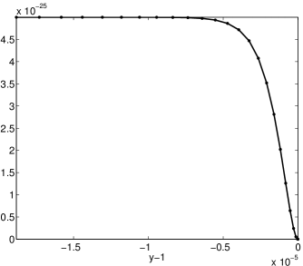
Figure 1.1: Very thin boundary layer at $y=1$ in the solution of the fourth order boundary value problem $(D^{2}-\beta^{2})(D^{2}-\alpha^{2})u=1$ with boundary conditions $u(\pm 1)=u^{\prime}(\pm 1)=0$ and with parameters $\alpha=10^{6}$ and $\beta=\sqrt{2}\alpha$. The solid markers are from an exact formula and the solid line is a numerical solution.

The channel geometry is rectangular with $x$, $y$, and $z$ being the streamwise, wall-normal, and spanwise directions by convention. The corresponding components of the velocity field $\mathbf{u}$ are denoted $u$, $v$, and $w$. The walls are at $y=\pm 1$ with fluid in between. The no-slip boundary conditions require $\mathbf{u}=0$ at $y=\pm 1$. The boundary conditions in the wall-parallel directions are typically periodic in numerical work. The flow is driven either by maintaining a constant mass flux or a constant pressure gradient in the streamwise direction. In plane Couette flow, the geometry is the same but the walls are moving. The no-slip boundary conditions are $(u,v,w)=(0,\pm 1,0)$ at $y=\pm 1$. Plane Couette flow is driven by the motion of the walls.

Both the Kleiser-Schumann and Kim-Moin-Moser methods come down to solving linear boundary value problems in the $y$ or wall-normal directions. The periodic directions are tackled using Fourier analysis and dealiasing of the nonlinear advection term. Each Fourier component then yields a linear boundary value problem in the $y$ direction. The $y$ direction is discretized using Chebyshev points $y_{j}=\cos j\pi/M$ with $j=0,\ldots,M$.

Here we parenthetically mention the interpretation of the parameters $\alpha$ and $\beta$, which occur in the ensuing discussion. The parameters are given by $\alpha^{2}=\ell^{2}/\Lambda_{x}^{2}+n^{2}/\Lambda_{z}^{2}$ and $\beta^{2}=\alpha^{2}+\gamma Re/\Delta t$, where $\ell$ and $n$ are the Fourier modes and $2\pi\Lambda_{x}$ and $2\pi\Lambda_{z}$ are the dimensions of the domain in the streamwise and spanwise directions, respectively. The parameter $\gamma$ depends on the time integration scheme. More details are found in Section 3.

In Figure 1.1, we have shown the solution of the linear boundary value problem

$$(D^{2}-\beta^{2})(D^{2}-\alpha^{2})u(y)=f(y)\quad\quad u(\pm 1)=u^{\prime}(\pm 1)=0$$ (1.1)

with $f(y)\equiv 1$. Here $D=\frac{d}{dy}$. A fourth order boundary value problem of this type occurs explicitly in the method of Kim-Moin-Moser but it is treated as a composition of two second order boundary value problems corresponding to the factors $D^{2}-\alpha^{2}$ and $D^{2}-\beta^{2}$. In the method of Kleiser-Schumann, a fourth order boundary value problem is not formed explicitly. Both methods solve the second order boundary value problem

$$(D^{2}-\beta^{2})u(y)=f(y)\quad\quad u(\pm 1)=0$$ (1.2)

by using the Chebyshev series $u(y)=\sum_{m=0}^{M}c_{m}T_{m}(y)$ and the set of equations obeyed by the coefficients $c_{n}$ given on page 119 of Gottlieb and Orszag [7, 1977].

Although the method on p. 119 of Gottlieb and Orszag [7] has been extensively used in turbulence computations for more than two decades, its numerical properties have not been investigated as far as we know. For reliable use in solving the Navier-Stokes equations at high Reynolds numbers, the method should be able to accurately reproduce thin boundary layers, such as the one shown in Figure 1.1. There is reason to be concerned. If the method is used to solve fourth order problems of the type (1.1), it forms linear systems with condition numbers of the order $\alpha^{2}\beta^{2}$ for the fourth order boundary value problem (1.1) and of order $\alpha^{2}$ for the second order boundary value problem (1.2) [31] . For the problem shown in Figure 1.1, the condition number is more than $10^{24}$ and greatly exceeds the machine epsilon of double precision arithmetic.

Zebib [34, 1984] and Greengard [8] suggested using a Chebyshev series for the highest derivative. For the fourth order problem (1.1), the Chebyshev expansion would be $u^{\prime\prime\prime\prime}=\sum_{m=0}^{M}c_{m}T_{m}(y)$. This device avoids the ill-conditioning of Chebyshev differentiation due to clustering at the end points that causes large errors in spectral differentiation. However, the spectral integration method of Zebib and Greengard also has a condition number greater than $\alpha^{2}\beta^{2}$ for the fourth order boundary value problem (1.1) [5, 31].

The method of spectral integration has been extended and investigated carefully in [31]. The equations presented somewhat tersely on p. 119 of Gottlieb and Orszag [7] are in fact a form of spectral integration. The methods used by Kleiser-Schumann and Kim-Moin-Moser have numerical properties that are practically identical to that of Zebib and Greengard. The essential equivalence of the Gottlieb-Orszag equations with spectral integration was first recognized by Charalambides and Waleffe [3]. Because of this equivalence the advantages of explicit spectral integration, as implemented in [18, 19] and [32], are not as overwhelming as illustrated in Figure 3 of [32]. When we refer to spectral integration, it includes the methods of Gottlieb-Orszag, Kleiser-Schumann, Zebib, Kim-Moin-Moser, and Greengard as well as the more general and powerful formulations derived in [31].

Regardless of which version of spectral integration is used, the fact remains that the linear system for the fourth order boundary value problem (1.1) has a condition number of $\alpha^{2}\beta^{2}$ . Yet, remarkably, even systems with condition numbers exceeding $10^{24}$ (see Figure 1.1) can be solved with a loss of only five or six digits of accuracy. The accuracy of spectral integration in spite of large condition numbers can be partly explained using the singular value decomposition [31]. Another property of spectral integration (in all its forms) is that some of the intermediate quantities have large errors which cancel in the final answer [31]. A robust implementation must take these two properties into account. Spectral integration can indeed handle thin boundary layers, such as the one shown in Figure 1.1, in spite of large condition numbers. The robustness of spectral integration was essential to the outstanding success of the methods of Kleiser-Schumann and Kim-Moin-Moser in more than two decades of use (however, not all implementations are equal).

In Figure 1.1, the thickness of the boundary layer is of the order $10^{-6}$. It takes more than $10,000$ Chebyshev points in the interval $-1\leq y\leq 1$ to resolve that boundary layer in spite of quadratic clustering near the endpoints. That is a lot more than the number needed if the grid points are chosen in a suitably adaptive manner. Viswanath [31] has derived a version of spectral integration that applies to piecewise Chebyshev grid points. Using that method, the number of grid points needed to solve a linear boundary value with a boundary layer as thin as the one shown in Figure 1.1 is reduced from $8192$ to $96$. It appears that this new method can be used to obtain considerable improvement in both the Kleiser-Schumann and Kim-Moin-Moser methods.

The Green’s function method, whose development we begin in this paper, is an alternative which in its final form will enjoy the same advantages. Spectral integration is an essentially one dimensional idea and cannot be generalized to pipe flows with non-circular cross-sections and to other non-rectangular geometries. The use of Green’s functions on the other hand will generalize. A great many analytic and numerical complications arise when Green’s functions are derived for cross-sections of pipes as a part of a numerical method for solving the Navier-Stokes equations. It is essential to develop the method for the channel geometry, as we do here, before those difficulties are confronted. It is also possible that the Green’s function method will turn out to be faster than the methods of Kleiser-Schumann and Kim-Moin-Moser, revised in the manner suggested in the previous paragraph, but one cannot be certain until the two alternatives are developed to their final form. Spectral integration over piecewise Chebyshev grids appears to be sensitive to the location of the nodes used to divided the interval [31]. The Green’s function method is likely to be much less sensitive. Lastly, we mention that the Green’s function method has a theoretical advantage. When implemented using suitable quadrature rules, its numerical stability is immediately obvious.

The Green’s function method for solving the Navier-Stokes equations in channel and plane Couette flow geometries is developed in Sections 2 and 3. The quadrature rule that is used is provisional. The way to derive robust quadrature rules is indicated in Section 3 and the complete method will be given in the sequel to this paper.

In Section 4, we show the theoretically intriguing result that Green’s functions may be used to eliminate numerical differentiation in the wall-normal or $y$ direction entirely from the numerical scheme. The derivatives that occur in the nonlinear advection term can be transferred to the Green’s function using integration by parts with the result that numerical differentiation is replaced by analytic differentiation. Such a scheme is not practical at high Reynolds numbers for reasons given in that section.

In Section 5, we validate the Green’s function based method. In view of the extensions discussed in this introduction, the code has been written in such a way that it can reach hundreds of millions of grid points using only a dozen or two processor cores. Since the piecewise Chebyshev extension with robust quadrature rules is yet to be fully developed, the full capabilities of this code are not exercised. Yet we report simulations with up to ten million grid points and investigate certain aspects of fully developed turbulence to demonstrate the viability of the Green’s function approach.

2 Green’s functions and template boundary value problems

Every time step in the solution of the Navier-Stokes equations in the channel geometry reduces to the solution of a number of linear boundary value problems of the type (1.1) and (1.2). In this section, we derive the Green’s functions for the solutions of those boundary value problems. The Green’s functions can be derived using very standard methods. However, the resulting expressions are unsuitable for numerical evaluation. When the parameters $\alpha$ and $\beta$ are as large as $10^{6}$, as in Figure 1.1, quantities of the type ${\rm e}^{\beta y}$ or ${\rm e}^{-\beta y}$ will overflow. Thus we begin by deriving the Green’s functions in a manner that leads to expressions suitable for accurate numerical evaluation. In the last part of this section, we consider the evaluation of derivatives such as $du/dy$, where $u$ is the solution of either of the boundary value problems (1.1) and (1.2), and the evaluation of the solution $u$ when the source term $f$ is given in the form $f\equiv df_{1}/dy$.

2.1 Green’s functions of linear boundary value problems

Let $Lu=u^{(n)}+a_{1}(y)u^{(n-1)}+\cdots+a_{n-1}(y)u^{(1)}+a_{n}(y)u$. The coefficients $a_{i}(y)$, $1\leq i\leq n$, are assumed to be real-valued and sufficiently smooth. The adjoint operator is given by $L^{+}v=(-1)^{n}v^{(n)}+(-1)^{n-1}(a_{1}v)^{(n-1)}+\cdots+a_{n}v$. We assume throughout that the functions that arise have the requisite order of smoothness and that $n\geq 2$. The degree of differentiability is specifically mentioned only if there is a nontrivial reason for doing so.

The lemmas in this subsection are not new. They can be found in [4] in some form or the other. However, our derivation leads to formulas which are easier to manipulate and which are suitable for numerical evaluation. Our derivation of the Green’s function for the boundary value problem $Lu=f$, $a\leq y\leq c$, with suitable boundary conditions on $u$, is based on the Lagrange identity, which is the next lemma.

Lemma 1.

For any two functions $u$ and $v$, the Lagrange identity $v\,Lu-u\,L^{+}v=[uv]^{\prime}$ holds, with

$$[uv]=\sum_{k=0}^{n-1}\sum_{r=0}^{n-k-1}(-1)^{r}(va_{k})^{(r)}u^{(n-k-r-1)}$$

and $a_{0}\equiv 1$.

Proof.

Begin with $\int v\,Lu\,dy$ and integrate each term by parts repeatedly. ∎

Define

$$\tilde{u}=\left(\begin{array}[]{c}u\\ u^{(1)}\\ \vdots\\ u^{(n-1)}\end{array}\right).$$

The quantity $[uv]$ which appears in the Lagrange identity may be written as $[uv]=\tilde{u}^{T}A\tilde{v}$, where $A$ is an $n\times n$ matrix. All the entries of $A$ are determined by the lemma. However, all that we need to know about $A$ is that it has the following reverse triangular structure

$$A=\left(\begin{array}[]{cccc}\cdot&\cdot&\cdot&(-1)^{n-1}\\ \cdot&\cdot&\cdot&0\\ \cdot&-1&0&0\\ 1&0&0&0\end{array}\right)$$

and that the reverse diagonal is as shown above.

Let $u_{1},\ldots,u_{n}$ be a basis of solutions of the homogeneous problem $Lu=0$. Similarly, let $v_{1},\ldots,v_{n}$ be a basis of solutions of the adjoint problem $L^{+}u=0$. Denote the $n\times n$ matrices

$$(\tilde{u}_{1},\ldots,\tilde{u}_{n})\quad\text{and}\quad(\tilde{v}_{1},\ldots,\tilde{v}_{n})$$

by $U$ and $V$, respectively (the determinant of $U$ is the Wronskian). The Lagrange identity implies the following lemma.

Lemma 2.

$\frac{d}{dy}\left(U^{T}AV\right)=0.$

We will assume that the bases of solutions are chosen in such a way that

$$U(y)^{T}A(y)V(y)=I$$ (2.1)

where $I$ is the identity matrix. The homogeneous solutions $u_{i}$ and $v_{i}$ are used to construct the Green’s function of $Lu=f$. Before deriving the Green’s function, we give the identity

$$v_{j}=\frac{\det\left(\begin{array}[]{cccc}u_{1}&\ldots&u_{1}^{(n-2)}&0\\ u_{2}&\ldots&u_{2}^{(n-2)}&\cdot\\ &\cdots&&1\\ &\cdots&&\cdot\\ u_{n}&\ldots&u_{n}^{(n-2)}&0\end{array}\right)}{\det\left(\begin{array}[]{cccc}u_{1}&u_{1}^{\prime}&\ldots&u_{1}^{(n-1)}\\ u_{2}&u_{2}^{\prime}&\ldots&u_{2}^{(n-1)}\\ &&\cdots\\ u_{n}&u_{n}^{\prime}&\ldots&u_{n}^{(n-1)}\end{array}\right)}.$$ (2.2)

The entry equal to $1$ in the last column of the numerator is in row number $j$. This identity is derived as follows. We choose the $j$-th column of (2.1) to get

$$U(y)^{T}A(y)\left(\begin{array}[]{c}v_{j}\\ \vdots\\ v_{j}^{(n-1)}\end{array}\right)=\left(\begin{array}[]{c}0\\ \vdots\\ 1\\ \vdots\\ 0\end{array}\right).$$

Because of the reverse triangular structure of $A$, the last entry of $A\tilde{v}_{j}$ is equal to $v_{j}$. Identity (2.2) is implied by Cramer’s rule. By working with rows of (2.1) instead of columns, we get the identity

$$u_{j}=(-1)^{n-1}\frac{\det\left(\begin{array}[]{cccc}v_{1}&\ldots&v_{1}^{(n-2)}&0\\ v_{2}&\ldots&v_{2}^{(n-2)}&\cdot\\ &\cdots&&1\\ &\cdots&&\cdot\\ v_{n}&\ldots&v_{n}^{(n-2)}&0\end{array}\right)}{\det\left(\begin{array}[]{cccc}v_{1}&v_{1}^{\prime}&\ldots&v_{1}^{(n-1)}\\ v_{2}&v_{2}^{\prime}&\ldots&v_{2}^{(n-1)}\\ &&\cdots\\ v_{n}&v_{n}^{\prime}&\ldots&v_{n}^{(n-1)}\end{array}\right)}.$$ (2.3)

The identities (2.2) and (2.3) are used to construct Green’s functions in Section 2.2.

So far, we have not specified the boundary conditions $u$ must satisfy in addition to $Lu=f$. We take the domain to be $a\leq y\leq c$ and require that $\tilde{u}(a)$ must lie in an $n-\ell$ dimensional subspace $V_{\ell}$ (this corresponds to $\ell$ linear conditions on $\tilde{u}(a)$). Similarly, the right boundary conditions require that $\tilde{u}(c)$ should lie in a $n-r$ dimensional subspace $V_{r}$. We require $\ell+r=n$. The Green’s function is built up using homogeneous solutions of $Lu=0$ which satisfy the left or the right boundary conditions. We assume that the basis solutions are chosen and then ordered in such a way that

$$\tilde{u}_{1}(c),\ldots,\tilde{u}_{\ell}(c)\quad\text{and}\quad\tilde{u}_{\ell+1}(a),\ldots,\tilde{u}_{n}(a)$$

span the subspaces $V_{r}$ and $V_{l}$, respectively. The following lemma gives the boundary conditions satisfied by $v_{1},\ldots,v_{n}$, a basis of solutions of $L^{+}v=0$ which is related to $u_{1},\ldots,u_{n}$ by (2.1). The lemma is useful for checking correctness of the implementation. It may also be used for the construction of $v_{i}$ given $u_{i}$. Its proof is obvious from $U^{T}AV=I$.

Lemma 3.

$\tilde{v}_{1}(a),\ldots,\tilde{v}_{l}(a)$ span the orthogonal complement of the $n-\ell$ dimensional space $A(a)^{T}V_{l}$ and $\tilde{v}_{l+1}(c),\ldots,\tilde{v}_{n}(c)$ span the orthogonal complement of the $n-r$ dimensional space $A(c)^{T}V_{r}$.

Let $u$ be the solution of $Lu=f$ subject to the boundary conditions $\tilde{u}(a)\in V_{\ell}$ and $\tilde{u}(b)\in V_{r}$. If we apply the Lagrange identity using $u$ and $v_{i}$, where $v_{i}$ is a solution of the homogeneous problem $L^{+}v=0$, we get $fv_{i}=\frac{d}{dy}\left(\tilde{u}^{T}Av_{i}\right)$ for $i=1,\ldots,n$. The equations with $i=1,\ldots,\ell$ are integrated from $a$ to $y$ and the rest are integrated from $y$ to $c$. The boundary conditions as given by the previous lemma imply that

$$\int_{a}^{y}fv_{1} = \tilde{u}(y)^{T}A(y)\tilde{v}_{1}(y)$$

$$\cdots$$

$$\int_{a}^{y}fv_{l} = \tilde{u}(y)^{T}A(y)\tilde{v}_{l}(y)$$

$$-\int_{y}^{c}fv_{l+1} = \tilde{u}(y)^{T}A(y)\tilde{v}_{l+1}(y)$$

$$\cdots$$

$$-\int_{y}^{c}fv_{n} = \tilde{u}(y)^{T}A(y)\tilde{v}_{n}(y).$$

The last entry of $A(y)^{T}\tilde{u}$ is equal to $(-1)^{n}u$. Using Cramer’s rule, we get

$$(-1)^{n-1}u=\frac{\det\left(\begin{array}[]{ccccc}v_{1}&v_{1}^{\prime}&\ldots&v_{1}^{(n-2)}&\int_{a}^{y}fv_{1}\\ &&\cdots\\ v_{n}&v_{n}^{\prime}&\ldots&v_{n}^{(n-2)}&-\int_{y}^{c}fv_{n}\end{array}\right)}{\det\left(\begin{array}[]{cccc}v_{1}&v_{1}^{\prime}&\ldots&v_{1}^{(n-1)}\\ v_{2}&v_{2}^{\prime}&\ldots&v_{2}^{(n-1)}\\ &&\cdots\\ v_{n}&v_{n}^{\prime}&\ldots&v_{n}^{(n-1)}\end{array}\right)}.$$ (2.4)

The following lemma gives the Green’s function in a more useful form.

Lemma 4.

The solution of $Lu=f$ subject to the boundary conditions $u(a)\in V_{\ell}$ and $u(c)\in V_{r}$ is given by

$$u(y)=u_{1}(y)\int_{a}^{y}v_{1}(\eta)f(\eta)\,d\eta+\cdots+u_{l}(y)\int_{a}^{y}v_{l}(\eta)f(\eta)\,d\eta\\ -u_{l+1}(y)\int_{y}^{c}v_{l+1}(\eta)f(\eta)\,d\eta-\cdots-u_{n}(y)\int_{y}^{c}v_{n}(\eta)f(\eta)\,d\eta.$$ (2.5)

Proof.

Use (2.3) and (2.4). ∎

The following lemma justifies the delta-function interpretation of Green’s functions favored by physicists. It is used in Section 2.3 and Section 4.

Lemma 5.

Let $u_{1},\ldots,u_{n}$ and $v_{1},\ldots,v_{n}$ be bases of solutions of the homogeneous problems $Lu=0$ and $L^{+}v=0$, respectively, that are related by $U(y)^{T}A(y)V(y)=I$. Then we have

$$\sum_{i=1}^{n}u_{i}^{(j)}v_{i} = 0\quad\text{for}\quad j=0,1,\ldots,n-2$$

$$= 1\quad\text{for}\quad j=n-1$$

and

$$\sum_{i=1}^{n}u_{i}v_{i}^{(j)} = 0\quad\text{for}\quad j=0,1,\ldots,n-2$$

$$= (-1)^{n-1}\quad\text{for}\quad j=n-1.$$

Proof.

Use (2.2) and (2.3). ∎

2.2 Template boundary value problems

The first template boundary value problem is

$$\left(D^{2}-\beta^{2}\right)u=f$$

with boundary conditions $u(\pm 1)=0$. The Green’s function of this boundary value can be deduced in any number of ways. We have

$$G(y,\eta)=\frac{-{\rm e}^{\beta\,\left(-2+y+\eta\right)}+{\rm e}^{-\beta\,\left(4-y+\eta\right)}+{\rm e}^{\beta\,\left(-y+\eta\right)}-{\rm e}^{-\beta\,\left(2+y+\eta\right)}}{2\,\beta\,\left({\rm e}^{-4\,\beta}-1\right)}$$ (2.6)

for $-1\leq\eta\leq y\leq 1$. The Green’s function is symmetric and the solution is given by $u(y)=\int_{-1}^{y}G(y,\eta)\,f(\eta)\,d\eta+\int_{y}^{\eta}G(\eta,y)\,f(\eta)\,d\eta.$ This form of the Green’s function suits numerical work because none of the terms will overflow for even $\beta$ very large. The terms in the numerator are factored as follows:

$${\rm e}^{\beta(-2+y+\eta)} ={\rm e}^{\beta(-1+y)}{\rm e}^{\beta(-1+\eta)}$$

$${\rm e}^{-\beta(4-y+\eta)} ={\rm e}^{-2\beta}{\rm e}^{-\beta(1-y)}{\rm e}^{-\beta(1+\eta)}$$

$${\rm e}^{-\beta(2+y+\eta)} ={\rm e}^{-\beta(1+y)}{\rm e}^{-\beta(1+\eta)}.$$

None of the factors will overflow even for large $\beta$. The term ${\rm e}^{\beta(-y+\eta)}$ is not factored and will not overflow because $\eta\leq y$. Using these factorizations and noting that $y$ and $\eta$ must be exchanged to get the Green’s function for $y\leq\eta$, we infer that the evaluation of the solution of the first template problem using $u=\int_{-1}^{y}G(y,\eta)\,f(\eta)\,d\eta+\int_{y}^{\eta}G(\eta,y)\,f(\eta)\,d\eta$ reduces to the quadratures

$$\int_{-1}^{y}{\rm e}^{-\mu(\eta+1)}f(\eta)\,d\eta,\>\int_{y}^{1}{\rm e}^{-\mu(\eta+1)}f(\eta)\,d\eta,\;\int_{-1}^{y}{\rm e}^{\mu(-1+\eta)}f(\eta)\,d\eta,\;\int_{y}^{1}{\rm e}^{\mu(-1+\eta)}f(\eta)\,d\eta$$ (2.7)

and

$$\int_{-1}^{+1}{\rm e}^{-\mu|y-\eta|}f(\eta)\,d\eta$$ (2.8)

with $\mu=\beta$. Each one of these quadratures yields a function of $y$ and must be multiplied by a prefactor which is also a function $y.$ For example, the first term of (2.6) contributes the prefactor $-{\rm e}^{\beta(-1+y)}/2\beta({\rm e}^{-4\beta}-1)$ to $\int_{-1}^{y}{\rm e}^{\beta(-1+\eta)}f(\eta)\,d\eta$. Since the term is unchanged when $y$ and $\eta$ are interchanged to obtain the Green’s function in $y\leq\eta$ region, it contributes the same prefactor to $\int_{y}^{1}{\rm e}^{\beta(-1+\eta)}f(\eta)\,d\eta$. The prefactor of the function defined by (2.8) with $\gamma=\beta$ is $1/2\beta({\rm e^{-4\beta}-1)}$. Unlike the result of the quadratures (2.7) and (2.8), the prefactors do not depend upon $f$ and can be computed and stored in advance. Thus the cost of solving the first template problem is very nearly equal to the cost of the quadratures (2.7) and (2.8) with $\gamma=\beta$.

The second template problem is the fourth order boundary value problem

$$\left(D^{2}-\beta^{2}\right)\left(D^{2}-\alpha^{2}\right)u=f$$

with boundary conditions $u(\pm 1)=u^{\prime}(\pm 1)=0$. For this problem, it takes more work to write the Green’s function in such a way that there are no numerical overflows even if $\alpha$ and $\beta$ are very large. However, the final result is similar to what we have seen for the first template problem. The evaluation of $u$ can be reduced to the quadratures (2.7) and (2.8) with $\gamma=\alpha$ and $\gamma=\beta$. The results of quadratures are multiplied by prefactors and summed to obtain $u$.

We now turn to the derivation of the $4\times 4$ matrix shown in Figure 2.1. That matrix is useful for computing the prefactors.

Like the first template problem, the second template problem is self-adjoint. We take the basis of homogeneous solutions to be

$$u_{1} ={\rm e}^{\beta\,\left(y-1\right)}+{\rm e}^{-\beta\,\left(y-1\right)}-{\rm e}^{\alpha\,\left(y-1\right)}-{\rm e}^{-\alpha\,\left(y-1\right)}$$

$$u_{2} =\alpha\,{{\rm e}^{\beta\,\left(y-1\right)}}-\alpha\,{{\rm e}^{-\beta\,\left(y-1\right)}}-\beta\,{{\rm e}^{\alpha\,\left(y-1\right)}}+\beta\,{{\rm e}^{-\alpha\,\left(y-1\right)}}$$

$$u_{3} ={{\rm e}^{\beta\,\left(y+1\right)}}+{{\rm e}^{-\beta\,\left(y+1\right)}}-{{\rm e}^{\alpha\,\left(y+1\right)}}-{{\rm e}^{-\alpha\,\left(y+1\right)}}$$

$$u_{4} =\alpha\,{{\rm e}^{\beta\,\left(y+1\right)}}-\alpha\,{{\rm e}^{-\beta\,\left(y+1\right)}}-\beta\,{{\rm e}^{\alpha\,\left(y+1\right)}}+\beta\,{{\rm e}^{-\alpha\,\left(y+1\right)}}.$$

It may be verified that $u_{1}$ and $u_{2}$ satisfy the right boundary conditions while $u_{3}$ and $u_{4}$ satisfy the left boundary conditions as assumed in Section 2.1. The functions $v_{1},v_{2},v_{3},v_{4}$ may be calculated using (2.2) or Lemma 3. It is convenient to define

$$W=-4\,\alpha\,\beta\,{\delta}^{2}{\sigma}^{2}{{\rm e}^{-4\,\alpha}}-4\,\alpha\,\beta\,{\delta}^{2}{\sigma}^{2}{{\rm e}^{-4\,\beta}}+4\,{\frac{\alpha\,\beta\,{\delta}^{4}{{\rm e}^{-4\,\beta-4\,\alpha}}}{{\sigma}^{2}}}+32\,{\alpha}^{2}{\beta}^{2}{\delta}^{2}{{\rm e}^{-2\,\beta-2\,\alpha}}+4\,{\frac{\alpha\,\beta\,{\delta}^{4}}{{\sigma}^{2}}}$$

where $\delta=\alpha^{2}-\beta^{2}$ and $\sigma=\alpha+\beta$ (the Wronskian is equal to ${\rm e}^{2\alpha+2\beta}W$). The function $v_{1}$ is equal to

$$2\,\alpha\,\beta\,\left(\beta+\alpha\right)\left(-\beta+\alpha\right)^{2}{{\rm e}^{\alpha\,\left(y-1\right)}}-2\,\alpha\,\beta\,\left(\beta+\alpha\right)\left(-\beta+\alpha\right)^{2}{{\rm e}^{\beta\,\left(y-1\right)}}+2\,\alpha\,\beta\,\left(-\beta+\alpha\right)\left(\beta+\alpha\right)^{2}{{\rm e}^{-\alpha\,\left(y+3\right)}}\\ +2\,\alpha\,\beta\,\left(-\beta+\alpha\right)\left(\beta+\alpha\right)^{2}{{\rm e}^{-\beta\,\left(y+3\right)}}+2\,\alpha\,\beta\,\left(\beta+\alpha\right)\left(-\beta+\alpha\right)^{2}{{\rm e}^{-4\,\alpha-\beta\,y-3\,\beta}}-2\,\alpha\,\beta\,\left(-\beta+\alpha\right)\left(\beta+\alpha\right)^{2}{{\rm e}^{-4\,\alpha+\beta\,y-\beta}}\\ -4\,{\alpha}^{2}\beta\,\left(-\beta+\alpha\right)\left(\beta+\alpha\right){{\rm e}^{-2\,\alpha-\beta\,y-\beta}}-2\,\alpha\,\beta\,\left(\beta+\alpha\right)\left(-\beta+\alpha\right)^{2}{{\rm e}^{-4\,\beta-\alpha\,y-3\,\alpha}}-2\,\alpha\,\beta\,\left(-\beta+\alpha\right)\left(\beta+\alpha\right)^{2}{{\rm e}^{-4\,\beta+\alpha\,y-\alpha}}\\ -4\,\alpha\,{\beta}^{2}\left(-\beta+\alpha\right)\left(\beta+\alpha\right){{\rm e}^{-2\,\beta-\alpha\,y-\alpha}}+4\,\alpha\,{\beta}^{2}\left(-\beta+\alpha\right)\left(\beta+\alpha\right){{\rm e}^{\alpha\,y-3\,\alpha-2\,\beta}}+4\,{\alpha}^{2}\beta\,\left(-\beta+\alpha\right)\left(\beta+\alpha\right){{\rm e}^{\beta\,y-3\,\beta-2\,\alpha}}$$

divided by $W$. The expression for $v_{2}$ is similarly long.

$$\left(\begin{array}[]{cccc}-2\,\alpha\,{\delta}^{2}+2\,\alpha\,{\delta}^{2}{{\rm e}^{-4\,\alpha}}&-8\,\beta\,{\alpha}^{2}\delta\,{{\rm e}^{-2\,\beta-2\,\alpha}}+2\,\alpha\,\delta\,{\sigma}^{2}{{\rm e}^{-4\,\alpha}}-2\,{\frac{\alpha\,{\delta}^{3}}{{\sigma}^{2}}}\\ 8\,\beta\,{\alpha}^{2}\delta\,{{\rm e}^{-2\,\alpha}}-2\,\alpha\,\delta\,{\sigma}^{2}{{\rm e}^{-2\,\beta}}+2\,{\frac{\alpha\,{\delta}^{3}{{\rm e}^{-4\,\alpha-2\,\beta}}}{{\sigma}^{2}}}&-2\,\alpha\,{\delta}^{2}+2\,\alpha\,{\delta}^{2}{{\rm e}^{-4\,\alpha}}\\ -4\,{\frac{\beta\,\alpha\,{\delta}^{2}{{\rm e}^{-2\,\beta-2\,\alpha}}}{\sigma}}+4\,{\frac{\beta\,\alpha\,{\delta}^{2}}{\sigma}}&-4\,\beta\,\alpha\,\delta\,\sigma\,{{\rm e}^{-2\,\alpha}}+4\,\beta\,\alpha\,\delta\,\sigma\,{{\rm e}^{-2\,\beta}}\\ -4\,\beta\,\alpha\,\delta\,\sigma\,{{\rm e}^{-2\,\alpha}}+4\,\beta\,\alpha\,\delta\,\sigma\,{{\rm e}^{-2\,\beta}}&-4\,{\frac{\beta\,\alpha\,{\delta}^{2}{{\rm e}^{-2\,\beta-2\,\alpha}}}{\sigma}}+4\,{\frac{\beta\,\alpha\,{\delta}^{2}}{\sigma}}\end{array}\right)$$

$$\left(\begin{array}[]{cccc}&&-4\,{\frac{\beta\,\alpha\,{\delta}^{2}{{\rm e}^{-2\,\beta-2\,\alpha}}}{\sigma}}+4\,{\frac{\beta\,\alpha\,{\delta}^{2}}{\sigma}}&-4\,\beta\,\alpha\,\delta\,\sigma\,{{\rm e}^{-2\,\alpha}}+4\,\beta\,\alpha\,\delta\,\sigma\,{{\rm e}^{-2\,\beta}}\\ &&-4\,\beta\,\alpha\,\delta\,\sigma\,{{\rm e}^{-2\,\alpha}}+4\,\beta\,\alpha\,\delta\,\sigma\,{{\rm e}^{-2\,\beta}}&-4\,{\frac{\beta\,\alpha\,{\delta}^{2}{{\rm e}^{-2\,\beta-2\,\alpha}}}{\sigma}}+4\,{\frac{\beta\,\alpha\,{\delta}^{2}}{\sigma}}\\ &&-2\,\beta\,{\delta}^{2}+2\,\beta\,{\delta}^{2}{{\rm e}^{-4\,\beta}}&8\,{\beta}^{2}\alpha\,\delta\,{{\rm e}^{-2\,\beta-2\,\alpha}}+2\,{\frac{\beta\,{\delta}^{3}}{{\sigma}^{2}}}-2\,\beta\,\delta\,{\sigma}^{2}{{\rm e}^{-4\,\beta}}\\ &&-8\,{\beta}^{2}\alpha\,\delta\,{{\rm e}^{-2\,\beta}}-2\,{\frac{\beta\,{\delta}^{3}{{\rm e}^{-4\,\beta-2\,\alpha}}}{{\sigma}^{2}}}+2\,\beta\,\delta\,{\sigma}^{2}{{\rm e}^{-2\,\alpha}}&-2\,\beta\,{\delta}^{2}+2\,\beta\,{\delta}^{2}{{\rm e}^{-4\,\beta}}\end{array}\right)$$

Figure 2.1: Entries of a $4\times 4$ matrix with the first two columns placed above the last two. This matrix determines the Green’s function of the second template problem. Here $\delta=\alpha^{2}-\beta^{2}$ and $\sigma=\alpha+\beta$.

For $\eta\leq y$, the Green’s function is given by $G(y,\eta)=u_{1}(y)v_{1}(\eta)+u_{2}(y)v_{2}(\eta).$ This Green’s function is determined by the $4\times 4$ matrix shown in Figure 2.1. We think of the rows and columns of the matrix as being indexed by $-\beta,\beta,-\alpha,\alpha$ in that order. The $(-\beta,-\beta)$ entry, which appears in the top left corner, is divided by $W$ to get the coefficient of ${\rm e}^{-\beta(y+1)}{\rm e}^{-\beta(\eta+1)}$ in the expression for $G(y,\eta)$ for $\eta\leq y$. The other entries are interpreted similarly but there are two special entries. These are the $(-\beta,\beta)$ entry which must be interpreted as $W$ times the coefficient of ${\rm e}^{\beta(\eta-y)}$ and the $(-\alpha,\alpha)$ entry which must be interpreted as $W$ times the coefficient of ${\rm e}^{\alpha(\eta-y)}$. The Green’s function for $y\leq\eta$ is obtained from symmetry.

It follows that solving the second template problem $\left(D^{2}-\beta^{2}\right)\left(D^{2}-\alpha^{2}\right)u=f$ with boundary conditions $u(\pm 1)=u^{\prime}(\pm 1)=0$ reduces to quadratures (2.7) and (2.8) with $\gamma=\alpha$ and $\gamma=\beta$. Each quadrature yields a function of $y$ which is multiplied by a prefactor. The prefactor is determined using the $4\times 4$ matrix of Figure 2.1 and the formula for $W$.

The formula for $W$ and the entries of the $4\times 4$ matrix use $\delta$ and $\sigma$ to avoid cancellation errors. Because of the way the parameters $\alpha$ and $\beta$ arise in the numerical integration of channel flow, $\delta=\alpha^{2}-\beta^{2}$ can be evaluated accurately.

Each of the quadratures (2.7) and (2.8) is well-conditioned. However, if $\alpha\approx\beta$ there will be large cancellation errors when the results of the quadratures are multiplied by prefactors and summed. This phenomenon may be understood as follows. When $\alpha\neq\beta$, the solutions ${\rm e}^{\pm\alpha y},{\rm e}^{\pm\beta y}$ form a basis of homogeneous solutions. When $\alpha=\beta$, the basis is ${\rm e}^{\pm\alpha y},y{\rm e}^{\pm\alpha y}$. When $\alpha\approx\beta$, the Green’s function tries to produce terms which resemble $y{\rm e}^{\alpha y}$ using terms such as $\left({\rm e}^{\alpha y}-{\rm e}^{\beta y}\right)/\left(\alpha-\beta\right)$ resulting in large cancellation errors. Fortunately, this situation does not arise in channel flow or plane Couette flow.

2.3 Derivatives using Green’s functions

For the template boundary value problems $Lu=f$, we have derived Green’s functions such that $u(y)=\int_{-1}^{1}G(y,\eta)\,f(\eta)\,d\eta$. Here we will consider the use of Green’s functions to evaluate derivatives such as $du/dy.$

The ability to differentiate solutions of boundary value problems using Green’s functions has been utilized in an important paper by Greengard and Rokhlin [9]. They consider the boundary value problem $u^{\prime\prime}+p(y)u^{\prime}+q(y)u=f(y)$ and solve it by representing the solution $u$ in the form $u=\int_{-1}^{1}G(y,\eta)\,\sigma(\eta)\,d\eta$, where $G$ is the Green’s function of a linear boundary value problem with constant coefficients which satisfies the same boundary conditions. In fact, the background boundary value problem is simply taken to be $u^{\prime\prime}=f$. With the representation of $u$ using $\sigma$, the boundary value problem becomes an integral equation for $\sigma$. Starr and Rokhlin [28] have generalized the method to first order systems. The papers by Greengard, Rokhlin, and Starr show how to apply numerical methods based on Green’s functions to problems with non-constant coefficients. Once the boundary value problem is cast in integral form using the background Green’s function, the method handles diagonal blocks using Nyström integration and pieces together the global solution efficiently by exploiting the low rank of the off-diagonal blocks.

We derive integral formulas for derivatives of solutions of both the second and fourth order template boundary value problems. In addition, we consider boundary value problems of the type $Lu=df_{1}/dy$ and $Lu=d^{2}f_{2}/dy^{2}$ and show how to get the solution $u$ as well as its derivatives without numerically differentiating $f_{1}$ or $f_{2}$. In Section 4, these calculations are used to show that numerical differentiation in the wall-normal or $y$ direction can be entirely eliminated in the numerical integration of channel flow.

For the template second order problem, which is $Lu=d^{2}u/dy^{2}-\beta^{2}u=f$ with boundaries $u(\pm 1)=0$, we take the Green’s function to be $G(y,\eta)=u_{1}(y)v_{1}(\eta)$ for $-1\leq\eta\leq y\leq 1$. The Green’s function for $-1\leq y\leq\eta\leq 1$ is taken to be $G(\eta,y)$ since the problem is symmetric or self-adjoint. The function $u_{1}$ satisfies the right boundary condition and the relationship between $u_{1},u_{2}$ and $v_{1},v_{2}$ is as given in Section 2.1. The Green’s function for $-1\leq y\leq\eta\leq 1$ is also given by $-u_{2}(y)v_{2}(\eta)$. As a consequence of symmetry, we have $-u_{2}(\eta)v_{2}(y)=u_{1}(y)v_{1}(\eta)$.

If $G(y,\eta)=u_{1}(y)v_{1}(\eta)$, we have $G_{1}(y,y)=G_{2}(y,y)+1$, where subscripts of $G$ denote partials with respect to the first or second argument. This follows from symmetry and Lemma 5. In addition, we have $G(1,y)=G(y,-1)=0$ because $u_{1}$ satisfies the right boundary condition and $v_{1}$ satisfies the left boundary condition.

The solution of $Lu=f$ is given by

$$u(y)=\int_{-1}^{y}G(y,\eta)\,f(\eta)\,d\eta+\int_{y}^{1}G(\eta,y)\,f(\eta)\,d\eta.$$ (2.9)

Differentiating with respect to $y$, we get

$$u^{\prime}(y)=\int_{-1}^{y}G_{1}(y,\eta)\,f(\eta)\,d\eta+\int_{y}^{1}G_{2}(\eta,y)\,f(\eta)\,d\eta$$ (2.10)

where subscripts of $G$ stand for partial differentiation. The integral equation is no longer symmetric in $y$ and $\eta$. Suppose the boundary value problem is $Lu=df_{1}/dy$. We may substitute $f_{1}^{\prime}$ for $f$ in (2.9) and integrate by parts to get

$$u(y)=-\int_{-1}^{y}G_{2}(y,\eta)\,f_{1}(\eta)\,d\eta-\int_{y}^{1}G_{1}(\eta,y)\,f_{1}(\eta)\,d\eta.$$ (2.11)

This integral equation for $u(y)$ is not symmetric. Differentiating with respect to $y$ and using $G_{1}(y,y)=G_{2}(y,y)+1$, we get

$$\frac{du}{dy}=-\int_{-1}^{y}G_{12}(y,\eta)\,f_{1}(\eta)\,d\eta-\int_{y}^{1}G_{12}(\eta,y)\,f_{1}(\eta)\,d\eta+f_{1}(y).$$ (2.12)

The template fourth order problem is $Lu=(D^{2}-\beta^{2})(D^{2}-\alpha^{2})u=f$ with boundary conditions $u(\pm 1)=u^{\prime}(\pm 1)=0$. We again take the Green’s function to be $G(y,\eta)$ for $-1\leq\eta\leq y\leq 1$. From Section 2.1, we have $G(y,\eta)=u_{1}(y)v_{1}(\eta)+u_{2}(y)v_{2}(\eta)$. Figure 2.1 gives the coefficients of the Green’s function as explained in Section 2.2. The functions $u_{1}(y)$ and $u_{2}(y)$ satisfy the right boundary condition. Using symmetry, we take the Green’s function for $-1\leq y\leq\eta\leq 1$ to be $G(\eta,y)$. As a consequence of symmetry, we have

$$u_{1}(y)v_{1}(\eta)+u_{2}(y)v_{2}(\eta)=-u_{3}(\eta)v_{3}(y)-u_{4}(\eta)v_{4}(y).$$

Using this identity and Lemma 5, we deduce that

$$G_{1}(y,y) =G_{2}(y,y)$$

$$G_{11}(y,y) =G_{22}(y,y)$$

$$G_{111}(y,y) =G_{222}(y,y)+1.$$

Here the subscripts of $G$ denote partial differentiation with $1$ and $2$ standing for the first and second arguments of $G$. Since $u_{1}$ and $u_{2}$ satisfy the right boundary conditions while $v_{1}$ and $v_{2}$ satisfy the left boundary conditions, we have

$$G(1,y)=G_{1}(1,y)=G(y,-1)=G_{2}(y,-1)=0.$$

In other words, the Green’s function satisfies the boundary conditions.

The solution of $Lu=f$, with the boundary conditions associated with the fourth order template problem, are given by

$$u(y)=\int_{-1}^{y}G(y,\eta)\,f(\eta)\,d\eta+\int_{y}^{1}G(\eta,y)\,f(\eta)\,d\eta$$ (2.13)

as before. Differentiating with respect to $y$ gives

$$\frac{du}{dy} =\int_{-1}^{y}G_{1}(y,\eta)\,f(\eta)\,d\eta+\int_{y}^{1}G_{2}(\eta,y)\,f(\eta)\,d\eta$$ (2.14)

$$\frac{d^{2}u}{dy^{2}} =\int_{-1}^{y}G_{11}(y,\eta)\,f(\eta)\,d\eta+\int_{y}^{1}G_{22}(\eta,y)\,f(\eta)\,d\eta.$$ (2.15)

The subscripts of $G$ denote differentiation. If the fourth order template problem is of the form $Lu=df_{1}/dy$, its solution is given by

$$u(y)=-\int_{-1}^{y}G_{2}(y,\eta)\,f_{1}(\eta)\,d\eta-\int_{y}^{1}G_{1}(\eta,y)\,f_{1}(\eta)\,d\eta.$$ (2.16)

This form of the solution is obtained after substituting $df_{1}/dt$ for $f$ in (2.13) and then integrating by parts. The boundary terms vanish. Differentiating with respect to $y$, we get

$$\frac{du}{dy} =-\int_{-1}^{y}G_{12}(y,\eta)\,f_{1}(\eta)\,d\eta-\int_{y}^{1}G_{12}(\eta,y)\,f_{1}(\eta)\,d\eta.$$ (2.17)

$$\frac{d^{2}u}{dy^{2}} =-\int_{-1}^{y}G_{112}(y,\eta)\,f_{1}(\eta)\,d\eta-\int_{y}^{1}G_{122}(\eta,y)\,f_{1}(\eta)\,d\eta.$$ (2.18)

The boundary terms vanish on both occasions. If the template fourth order boundary value problem is in the form $Lu=d^{2}f_{2}/dy^{2}$, the analogous formulas are as follows:

$$u(y) =\int_{-1}^{y}G_{22}(y,\eta)\,f_{2}(\eta)\,d\eta+\int_{y}^{1}G_{11}(\eta,y)\,f_{2}(\eta)\,d\eta$$

$$\frac{du}{dy} =\int_{-1}^{y}G_{122}(y,\eta)\,f_{2}(\eta)\,d\eta+\int_{y}^{1}G_{112}(\eta,y)\,f_{2}(\eta)\,d\eta$$

$$\frac{d^{2}u}{dy^{2}} =\int_{-1}^{y}G_{1122}(y,\eta)\,f_{2}(\eta)\,d\eta+\int_{y}^{1}G_{1122}(\eta,y)\,f_{2}(\eta)\,d\eta+(G_{122}(y,y)-G_{112}(y,y))\,f_{2}(y).$$ (2.19)

These formulas are derived using the properties of $G$ given in the previous paragraph.

Formulas (2.9) through (2.19) give a method to compute solutions and solution derivatives without numerical differentiation even when the right hand side of the boundary value problem is given as a derivative. If the right hand is $df_{1}/dy$, these formulas use $f_{1}$ and not $df_{1}/dy$. The derivatives are transferred to the Green’s function which can be differentiated analytically. In the case of the template fourth order problem, the kernels of the formulas can be described using a matrix such as the one displayed in Figure 2.1. In fact the kernels can be obtained by multiplying the entries of that matrix with suitable powers of $\alpha$ and $\beta.$ With such a representation the kernels can be evaluated in a numerically stable way as described in Section 2.2.

The numerical evaluation of formulas (2.9) through (2.19) is affected by discretization and rounding errors in varying ways. To avoid writing down long formulas, we limit the discussion of numerical errors to the template second order problem and note that very similar issues arise for the template fourth order boundary value problem.

When the integral formulation is used, the solution of the template second order problem $(D^{2}-\beta^{2})u=f$ at the boundary point $y=1$ is obtained as the sum of the following four terms:

$$\int_{-1}^{1}\frac{\mathrm{e}^{\beta(\eta-1)}f(\eta)}{2\beta(1-{\rm e}^{-4\beta})}\,d\eta,\int_{-1}^{1}\frac{{\rm e}^{-2\beta}{\rm e}^{-\beta(\eta+1)}f(\eta)}{2\beta(1-{\rm e}^{-4\beta})}\,d\eta,-\int_{-1}^{1}\frac{{\rm e}^{-2\beta}{\rm e}^{-\beta(\eta+1)}\,f(\eta)}{2\beta(1-{\rm e}^{-4\beta})}\,d\eta,-\int_{-1}^{1}\frac{{\rm e}^{\beta(\eta-1)}\,f(\eta)}{2\beta(1-{\rm e}^{-4\beta})}\,d\eta.$$ (2.20)

The second and third terms are exceedingly small even for moderate $\beta$. The main contribution to numerical error is from the exact cancellation between the first and the last terms. The magnitude of the first or the last term is of the order $\left|f\right|_{\infty}/\beta^{2}$. If the quadrature rule is a very good one, each of the integrals may be evaluated with an error of around $\left|f\right|_{\infty}\beta^{-2}\epsilon_{machine}$. If such a quadrature rule is devised, the error in the boundary layer will also be of the same order. If we suppose $f\equiv\beta^{2}$, then the exact formula will look like $1-{\rm e}^{\beta(y-1)}$ near the $y=1$. Since $1$ is a special number in machine arithmetic, the subtraction $y-1$ will be exact at $y=1$ but not at other nearby points. If we take the subtraction error at $y=1$ to follow the same model as at other points, we get the error in the boundary layer using the exact formula to be of the order $\left|1-{\rm e}^{\beta\epsilon}\right|\approx\beta\epsilon$ or $\left|f\right|_{\infty}\epsilon_{machine}/\beta$. Thus the integral form has the potential to be more accurate in the boundary layer than even the mathematically exact formula. Here we envisage quadrature rules for the sort of integrals that occur in (2.20) which take into account the occurrence of terms such as ${\rm e}^{-\beta(\eta+1)}$ in the integrands and whose weights and nodes are computed using extended precision.

The use of formulas such as (2.10) to compute the derivative $du/dy$ is especially accurate in the boundary layer. For instance, at $y=1$ the first term of (2.20) gets multiplied by $\beta$ and the last term by $-\beta$ with the result that there is no cancellation error in the boundary layer. In view of this observation, some of the errors reported in Table 7 of [9] may appear a little high for the function derivative.

Finally, we consider a type of numerical error that arises in formulas such as (2.16) that express the solution of $Lu=df_{1}/dy$ in integral form without differentiation of $f_{1}$. If $\beta$ is large in the template second order problem $(D^{2}-\beta^{2})u=f$, the solution satisfies $u\approx-f/\beta^{2}$ away from the boundary. Thus if $f$ is given in the form $df_{1}/dy$, the solution will satisfy $u\approx-\frac{df_{1}}{dy}\beta^{-2}$ and a formula such as (2.16) essentially has to produce the derivative of $f_{1}$ away from the boundary using integration. Differentiation is defined by subtracting nearly equal quantities and the cancellation errors inherent in that process cannot go away entirely. The same comment applies to formulas such as (2.10) which produce solution derivatives using an integral formula or to the evaluation of solution derivatives using the background Green’s function as in [9] or to the method of spectral integration discussed in the introduction. The principle contribution to the solution of $(D^{2}-\beta^{2})u=f$ for large $\beta$ and away from the boundary is due to the term

$$\frac{1}{2\beta({\rm e}^{-4\beta}-1)}\int_{-1}^{1}{\rm e}^{-\beta|\eta-y|}\,f(\eta)\,d\eta.$$

This is the term which makes the solution look like $-f\beta^{-2}$ away from the boundary. When (2.10) is used to evaluate $du/dy$ with $u$ being the solution of $Lu=f$, the leading contribution is from the two terms

$$\frac{1}{2\beta({\rm e}^{-4\beta}-1)}\left(\int_{-1}^{y}{\rm e}^{\beta(\eta-y)}\,f(\eta)\,d\eta-\int_{y}^{1}{\rm e}^{\beta(y-\eta)}\,f(\eta)\,d\eta\right).$$

Here the cancellation error we are looking for is evident. A numerical method that uses integral formulas to evaluate solution derivatives or to eliminate derivatives that appear on the right hand side would benefit by treating such terms together, especially when quadrature rules are derived.

3 Time integration of the Navier-Stokes equations

Let ${\bf u}=(u,v,w)$ be the velocity field of channel flow or plane Couette flow. We assume the domain to be periodic in the wall-parallel directions with periods equal to $2\pi\Lambda_{x}$ and $2\pi\Lambda_{z}$ in the streamwise and spanwise directions, respectively. The Fourier decomposition of the velocity field is given by

$${\bf u}=\sum_{\ell=-L/2}^{L/2}\sum_{n=N/2}^{N/2}\hat{{\bf u}}_{\ell,n}(y){\rm e}^{i\ell x/\Lambda_{x}+inz/\Lambda_{z}}.$$

This Fourier decomposition assumes the number grid points in the streamwise and spanwise directions to be $L$ and $N$. The notation $\hat{{\bf u}}_{\ell,n}$ denotes a Fourier coefficient of the entire velocity field. Similarly, $\hat{u}_{\ell,n}$, $\hat{v}_{\ell,n}$, $\hat{w}_{\ell,n}$ denote the Fourier coefficients of the streamwise, wall-normal, and spanwise components of the velocity field, respectively. The components of the vorticity $\nabla\times{\bf u}$ are denoted by $\omega_{x},\,\omega_{y},\,\omega_{z}$ and their Fourier components are denoted similarly.

Often which modes $\ell$ and $n$ apply is clear from context and the Fourier modes are indicated as $\hat{u}$, $\hat{v}$, $\hat{w}$ without subscripts. The $\ell=n=0$ modes are the mean modes and are denoted using an over-bar. For example, the mean mode of the streamwise velocity is $\bar{u}$. In both the flows considered here, the range of the $y$ variable is $-1\leq y\leq 1$, with the walls located at $y=\pm 1$.

3.1 The Kim-Moin-Moser equations

We take the Navier-Stokes equations to be $\partial{\bf u}/\partial t+{\bf H}=-\nabla p+\triangle{\bf u}/Re$, with ${\bf H}=(H_{1},H_{2},H_{3})$ being the nonlinear term. Both the Kleiser-Schumann [14]and Kim-Moin-Moser [13] methods begin by substituting the truncated Fourier expansion of the velocity field ${\bf u}$. The various Fourier modes are coupled through the nonlinear term. The nonlinear term is dealiased using the $3/2$ rule [2].

Both the methods use identical equations for the mean streamwise velocity and mean spanwise velocity:

$$\frac{\partial\bar{u}}{\partial t}=-\bar{H}_{1}+p_{g}+\frac{1}{Re}\frac{\partial^{2}\bar{u}}{\partial y^{2}}\quad\quad\quad\frac{\partial\bar{w}}{\partial t}=-\bar{H}_{3}+\frac{1}{Re}\frac{\partial^{2}\bar{w}}{\partial y^{2}}$$ (3.1)

For plane Couette flow $p_{g}=0$ and the boundary conditions are $\bar{u}(\pm 1)=\pm 1$ and $\bar{w}(\pm 1)=0$. For channel flow, $\bar{u}(\pm 1)=\bar{w}(\pm 1)=0$ but $p_{g}$ is non-zero. We may take $p_{g}=2/Re$ and maintain a constant pressure gradient or we may take

$$p_{g}=\frac{1}{2}\int_{-1}^{+1}\bar{H}_{1}\,dy-\frac{1}{2Re}\frac{\partial\bar{u}}{\partial y}\Biggl{|}_{y=-1}^{y=1}$$ (3.2)

and keep the streamwise mass flux $\frac{1}{2}\int_{-1}^{+1}\bar{u}\,dy$ constant at $2/3$. The laminar solution of channel flow is ${\bf u}=(1-y^{2},0,0)$ in both cases.

The equations for the $(\ell,n)$ mode are

$$\frac{\partial\hat{u}}{\partial t}+\hat{H}_{1} =-\left(\frac{i\ell}{\Lambda_{x}}\right)\hat{p}+\left(D^{2}-\frac{\ell^{2}}{\Lambda_{x}^{2}}-\frac{n^{2}}{\Lambda_{z}^{2}}\right)\hat{u}$$

$$\frac{\partial\hat{v}}{\partial t}+\hat{H}_{2} =-\frac{\partial\hat{p}}{\partial y}+\left(D^{2}-\frac{\ell^{2}}{\Lambda_{x}^{2}}-\frac{n^{2}}{\Lambda_{z}^{2}}\right)\hat{v}$$

$$\frac{\partial\hat{w}}{\partial t}+\hat{H}_{3} =-\left(\frac{in}{\Lambda_{z}}\right)\hat{p}+\left(D^{2}-\frac{\ell^{2}}{\Lambda_{x}^{2}}-\frac{n^{2}}{\Lambda_{z}^{2}}\right)\hat{w}.$$

Here all the hatted variables are Fourier coefficients of the $(\ell,n)$ mode and are functions of $y$. As before $D$ denotes $d/dy$. The incompressibility constraint $\nabla.{\bf u}=0$ gives $i\ell\hat{u}/\Lambda_{x}+\partial\hat{v}/\partial y+in\hat{w}/\Lambda_{z}=0$. The equations are solved in this form by the Kleiser-Schumann method. In the Kim-Moin-Moser method these equations are altered to

$$\frac{\partial\hat{\omega_{y}}}{\partial t}+\hat{H}_{4} =\frac{1}{Re}\left(D^{2}-\frac{\ell^{2}}{\Lambda_{x}^{2}}-\frac{n^{2}}{\Lambda_{z}^{2}}\right)\hat{\omega_{y}}$$

$$\frac{\partial}{\partial t}\left(D^{2}-\frac{\ell^{2}}{\Lambda_{x}^{2}}-\frac{n^{2}}{\Lambda_{z}^{2}}\right)\hat{v}+\hat{H}_{5} =\frac{1}{Re}\left(D^{2}-\frac{\ell^{2}}{\Lambda_{x}^{2}}-\frac{n^{2}}{\Lambda_{z}^{2}}\right)^{2}\hat{v}.$$ (3.3)

The boundary conditions are $\hat{\omega_{y}}(\pm 1)=\hat{v}(\pm 1)=\frac{d\hat{v}}{dy}(\pm 1)=0$. Here

$$H_{4}=\frac{\partial H_{1}}{\partial z}-\frac{\partial H_{3}}{\partial x}\quad\text{and}\quad H_{5}=\frac{\partial^{2}H_{2}}{\partial x^{2}}+\frac{\partial^{2}H_{2}}{\partial z^{2}}-\frac{\partial^{2}H_{1}}{\partial y\partial x}-\frac{\partial^{2}H_{3}}{\partial y\partial z}.$$

The entire velocity field can be recovered using $\bar{u}$, $\bar{w}$, $\omega_{y}$, and $v$ [13].

Imposing physically correct boundary conditions on pressure causes some complications and is a potential pitfall. Early discussions of this issue are found in [14, 20]. A thorough discussion of this topic, important both for mathematical theory and for computation, is found in an illuminating paper by Rempfer [24].

3.2 Time stepping using Green’s functions

If the Kim-Moin-Moser equations (3.1) and (3.3) are discretized in time, we get linear boundary value problems in the wall-normal or $y$ direction. Green’s functions will be used to solve these linear boundary value problems. An advantage of this method is that the boundary layers are analytically built into the Green’s functions.

The original paper by Kim, Moin, and Moser [13] used the CNAB (Crank-Nicolson and Adam-Bashforth) discretization in time. If the method is applied to the $\hat{\omega}_{y}$ equation in (3.3), we get

$$\frac{\hat{\omega}_{y}^{n+1}-\hat{\omega}_{y}^{n}}{\Delta t}=-\frac{3\hat{H}_{4}^{n}-\hat{H}_{4}^{n-1}}{2}+\frac{1}{Re}\left(D^{2}-\frac{\ell^{2}}{\Lambda_{x}^{2}}-\frac{n^{2}}{\Lambda_{z}^{2}}\right)\left(\frac{\hat{\omega}_{y}^{n+1}+\hat{\omega}_{y}^{n}}{2}\right).$$

The superscripts denote time steps. It is well-known that the numerical stability of Crank-Nicolson can be dicey in spite of its stability region being the entire left half plane. The eigenvalue equal to $\lambda$ corresponds to an amplification factor of $(1+\lambda\Delta t)/(1-\lambda\Delta t)$. The amplification is by a factor less than $1$ in magnitude for eigenvalues with a negative real part. However, the amplification factor can be very close to $1$ for eigenvalues such as $\lambda=-10^{10}$ which correspond to rapid decay. If care is taken to use the same scheme for differentiating $\hat{\omega}_{y}^{n+1}$ and $\hat{\omega}_{y}^{n}$, or if the boundary value problem is solved for $\hat{\omega}_{y}^{n+1}+\hat{\omega}_{y}^{n}$ at each time step, CNAB will be stable. We found it difficult to stabilize CNAB for the $\hat{v}$ equation in (3.3). This could be because we are mixing integration using a Green’s function with the second derivative that comes from the left hand side of (3.3), or it could be because the best possible quadrature rules for this problem are yet to be derived. We will not consider CNAB any further.

Suppose $dX/dt=f(X)+\triangle X/Re$, where $f(X)$ is a nonlinear term. The time discretizations we consider are of the following form:

$$\frac{1}{\Delta t}\left(\gamma X^{n+1}+\sum_{j=0}^{s-1}a_{j}X^{n-j}\right)=\sum_{j=0}^{s-1}b_{j}f(X^{n-j})+\frac{1}{Re}\triangle X^{n+1}.$$

If the $\bar{u}$ equation of (3.1) is discretized in time, it fits the template second order boundary value problem $(D^{2}-\beta^{2})u=f$ with

$$u=\bar{u}^{n+1},\quad\beta^{2}=\frac{\gamma Re}{\Delta t},\quad f=\frac{Re}{\Delta t}\sum_{j=0}^{s-1}a_{j}\bar{u}^{n-j}+Re\sum_{j=0}^{s-1}(\bar{H}_{1}^{n-j}-p_{g}^{n+1}).$$ (3.4)

The time discretization of the $\bar{w}$ equation of (3.1) fits the template second order boundary value problem $(D^{2}-\beta^{2})u=f$ with

$$u=\bar{w}^{n+1},\quad\beta^{2}=\frac{\gamma Re}{\Delta t},\quad f=\frac{Re}{\Delta t}\sum_{j=0}^{s-1}a_{j}\bar{w}^{n-j}+Re\sum_{j=0}^{s-1}H_{3}^{n-j}.$$ (3.5)

The time discretization of the $\hat{\omega}_{y}$ equation of (3.3) also fits the template second order boundary value problem:

$$u=\hat{\omega}_{y}^{n+1},\quad\beta^{2}=\frac{\ell^{2}}{\Lambda_{x}^{2}}+\frac{n^{2}}{\Lambda_{z}^{2}}+\frac{\gamma Re}{\Delta t},\quad f=\frac{Re}{\Delta t}\sum_{j=0}^{s-1}a_{j}\hat{\omega}_{y}^{n-j}+Re\sum_{j=0}^{s-1}b_{j}\hat{H}_{4}^{n-j}.$$ (3.6)

The time discretization of the $\hat{v}$ equation of (3.3) fits the template fourth order boundary value problem (1.1) as follows:

$$u=\hat{v}^{n+1},\quad\alpha^{2}=\frac{\ell^{2}}{\Lambda_{x}^{2}}+\frac{n^{2}}{\Lambda_{z}^{2}},\quad\beta^{2}=\alpha^{2}+\frac{\gamma Re}{\Delta t},\quad f=\frac{Re}{\Delta t}\sum_{j=0}^{s-1}a_{j}(D^{2}-\alpha^{2})\hat{v}^{n-j}+Re\sum_{j=0}^{s-1}b_{j}\hat{H}_{5}^{n-j}.$$ (3.7)

From the manner in which $\alpha^{2}$ and $\beta^{2}$ arise, the advantage of casting the Green’s function for the template fourth order problem using $\delta=\alpha^{2}-\beta^{2}$ and $\sigma=\alpha^{2}+\beta^{2}$ , as we did in Figure 2.1 and Section 2.2, is evident. Both $\delta$ and $\sigma$ can be evaluated without cancellation errors.

The equations (3.4), (3.5), (3.6), and (3.7) are reduced to quadratures of the type (2.7) and (2.8) as explained in Section 2. In the fourth order problem (3.7), which is solved for $\hat{v}^{n+1}$, the right hand side uses second derivatives of $\hat{v}^{n-j}$ from previous stages. The calculation of this second derivative is reduced to quadratures using (2.14).

The time stepping schemes we have implemented use

$$s=1,\,\gamma=1,\,a_{1}=-1,\,b_{1}=1$$

$$s=2,\,\gamma=3/2,\,a_{1}=-2,\,a_{2}=1/2,\,b_{1}=2,\,b_{2}=-1$$

$$s=2,\,\gamma=11/6,\,a_{1}=-3,\,a_{2}=3/2,\,a_{3}=-1/3,\,b_{1}=3,\,b_{2}=-3,\,b_{3}=1.$$

These are implicit-explicit multistep schemes that correspond to backward Euler, BDF2, and BDF3 respectively. For derivations of these schemes, see [1, 6, 30].

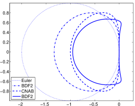
Figure 3.1: Absolute stability regions of the explicit halves of the implicit-explicit methods based on backward Euler, CNAB, BDF2, and BDF3.

The absolute stability regions of the explicit halves of some time integration schemes are shown in Figure 3.1 for reference. In turbulence simulations, the nonlinear advection term, which is discretized using an explicit scheme, is more of a constraint on the time step than the diffusion term which is handled implicitly. The discretization of the viscous diffusion term is by itself unconditionally stable.

To complete the description of these methods, we need to explain the method that is used to solve the quadrature problems (2.7) and (2.8) numerically. These quadrature problems are extremely well-conditioned even for large $\mu$. The method that is currently implemented for (2.7) expands the integrand in a Chebyshev series and integrates the terms of the series using well-known formulas. A better method would be to obtain quadrature nodes and weights for weighted integrals with weight functions equal to ${\rm e}^{\pm\mu(t\mp 1)}$, evaluate the other factor $f(t)$ at the nodes using an accurate and efficient interpolation algorithm, and sum using the quadrature weights. Such a method will be developed in future research. The current method develops spurious difficulties when $\mu$ is large, although it is good enough to allow us to exhibit simulations of fully developed turbulence in Section 5. In addition, if the idea of representing functions using piecewise Chebyshev collocation, which is briefly mentioned in the introduction and discussed at greater length in the context of spectral integration in [31], is employed, even the basic quadrature that is now implemented is likely to be adequate, even for very large $\mu$. The Green’s functions of Section 2 are completely independent of the discretization used in the wall-normal or $y$ direction. The discretization could be Chebyshev, or piecewise Chebyshev, or something else. The ease with which piecewise Chebyshev discretization can be incorporated into numerical methods that use Green’s functions was one of our prime motivations. At the moment, the quadrature problem (2.8) is solved numerically using spectral integration. Similar comments apply to this quadrature problem as well.

In direct numerical simulation of turbulence it is more common to use explicit-implict Runge-Kutta methods in the direct numerical simulation of turbulence [11, 21, 23, 27]. The advantanges of Runge-Kutta are ease of initialization and the possibility of adaptive time-stepping with embedded pairs. In the solution of ordinary differential equations, multistep methods and Runge-Kutta methods have been compared extensively [10]. It is now known that multistep methods can be initialized and time stepped adatively with equal effectiveness. This technology will be carried over to implicit-explicit multistep formulas in future research. Here we have preferred multistep formulas partly in order to leave room for this future research. Runge-Kutta methods typically have larger stability region but with each step costing more function evaluations. In future research, we will show how to derive implicit-explicit multistep methods with stability regions that are particularly advantageous for problems such as high $Re$ turbulence simulations.

4 A discrete model without spatial differentiation

Here we explain how numerical differentiation in the wall-normal or $y$ direction can be completely eliminated by employing the divergence form of the nonlinear term.

The Kim-Moin-Moser equation for $\bar{u}$ given in (3.1) has an $\bar{H}_{1}$ term. The nonlinear term $H_{1}$ is given by $H_{1}=\partial_{x}(u^{2})+\partial_{y}(uv)+\partial_{z}(uw)$. So we may take $\bar{H}_{1}=\partial_{y}\bar{uv}$. The mean mode $\bar{u}$ is advanced in time by solving the boundary value problem (3.4). The right hand side of the template boundary value problem is taken to be $f$, where $f$ is given by (3.4). The $\bar{H_{1}}$ terms in that right hand side may be removed and a new right hand side written as $df_{1}/dy$ introduced in their place. The contribution of a given time step to $f_{1}$ is taken to be $Re$ times $\bar{uv}$ evaluated at that time step. These contributions are weighted by $b_{j}$ and combined as before. The mean mode $\bar{u}$ is advanced in time using (2.9) and (2.16) and its derivative, if needed in (3.2), is calculated using (2.10) and (2.12).

The $\bar{w}$ and $\hat{\omega}_{y}$ equations are treated similarly. The $\hat{\omega}_{y}$ equation in (3.3) has an $\hat{H}_{4}$ term. The terms of $H_{4}$ that do not require differentiation in $y$ are

$$\frac{\partial^{2}u^{2}}{\partial x\partial z}+\frac{\partial^{2}uw}{\partial z^{2}}-\frac{\partial^{2}uw}{\partial x^{2}}-\frac{\partial^{2}w^{2}}{\partial x\partial z}$$

and the terms which require a single differentiation are

$$\frac{\partial^{2}uv}{\partial y\partial z}-\frac{\partial^{2}vw}{\partial x\partial y}.$$

These terms are separated and some of them are removed from the $f$ given in (3.6) and a new term $df_{1}/dy$ is inserted in the right hand side.

The treatment of $\hat{v}$ modes is a bit more elaborate. The right hand side $H_{5}$ may be written as

$$\left(\frac{\partial^{3}(uv)}{\partial x^{3}}+\frac{\partial^{3}(uv)}{\partial x\partial z^{2}}+\frac{\partial^{3}(vw)}{\partial x^{2}\partial z}+\frac{\partial^{3}(vw)}{\partial z^{3}}\right)+\left(\frac{\partial^{3}(v^{2})}{\partial x^{2}\partial y}+\frac{\partial^{3}(v^{2})}{\partial y\partial z^{2}}-\frac{\partial^{3}(u^{2})}{\partial x^{2}\partial y}-2\frac{\partial^{3}(uw)}{\partial x\partial y\partial z}-\frac{\partial^{3}(w^{2})}{\partial y\partial z^{2}}\right)\\ +\left(-\frac{\partial^{3}(uv)}{\partial x\partial y^{2}}-\frac{\partial^{3}(vw)}{\partial y^{2}\partial z}\right),$$

where terms are grouped depending upon whether they require zero, one, or two differentiations with respect to $y.$ The right hand side of the template fourth order problem which is given as $f$ in (3.7) may be rewritten as $f+df_{1}/dy+d^{2}f_{2}/dy^{2}$, with none of $f$, $f_{1}$, and $f_{2}$ involving differentiation with respect to $y$. The integral equations (2.13) through (2.19) may be used to produce $\hat{v}$, $d\hat{v}/dy$, and even $d^{2}\hat{v}/dy^{2}$. The first derivative $d\hat{v}/dy$ is needed when the full velocity field is reconstructed from $\bar{u}$, $\bar{w}$, and the modes $\hat{\omega}_{y}$ and $\hat{v}$ [13]. Turning this into a practical method hinges on numerical issues discussed at the end of Section 2. Eliminating numerical differentiation with respect to $y$ may be useful if a large number of Chebyshev points is used in the $y$ direction. However, it appears that piecewise Chebyshev grids can resolve boundary layers and internal layers while using only a small number of Chebyshev points in each sub-interval. Handling piecewise Chebyshev grids after reducing each time step to quadratures of the form (2.7) and (2.8) is as easy as $\int_{a}^{c}=\int_{a}^{b}+\int_{b}^{c}$. In piecewise Chebyshev grids, numerical errors due to differentiation are not a cause for concern.

5 Numerical validation

The numerical method described in Section 3 for solving the incompressible Navier-Stokes equations has been implemented and tested in numerous ways. Many earlier computations of plane Couette flow and channel flow have been reproduced with precision. In this section, we describe a few computations of fully developed turbulence. All the computations described here are for channel flow. Channel flow is used far more often than plane Couette flow in turbulence simulations.

A useful summary of turbulence computations of channel flow is given by Toh and Itano [29]. The Reynolds number $Re$ by itself is not a good metric to assess the difficulty of a turbulence computation because simple solutions such as the laminar solution can be computed easily at any Reynolds number. The metric must take into account both the Reynolds number and the kind of solutions that the simulation generates. One useful metric is obtained by taking the time average of $d\bar{u}/dy$ at the walls, where $\bar{u}$ is the mean streamwise velocity, and then computing $Re_{\tau}=\sqrt{Re\times|d\bar{u}/dy|}$. The frictional Reynolds number $Re_{\tau}$ is a good measure of the difficulty of the simulation. The highest $Re_{\tau}$ reached appears to be $2000$ in the work of Hoyas and Jimenez[11]. The lowest $Re_{\tau}$ at which one still observe turbulence appears to be around $100$ [12]. Nikitin [22, 23] has derived a method for solving the incompressible Navier-Stokes equations in orthogonal curvilinear coordinates. Nikitin’s method uses staggered grids, centered differences, cell averages for nonlinear terms, and explicit projections to enforce the incompressibility condition. The same program can handle channel, pipe, eccentric pipe and other geometries. Nikitin’s method has been used to simulate fully developed turbulence at an $Re_{\tau}$ of $500$.

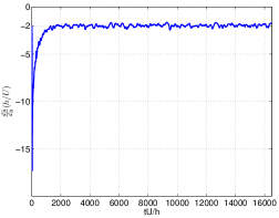
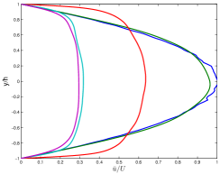
Figure 5.1: The first plot shows the variation of the mean shear at the wall as a function of time. The second plot shows the evolution of the mean flow during transition to turbulence. Units are given in terms of channel half-width $h$ and laminar center-line velocity $U$.

Prior to numerical validation, we discuss the pressure boundary condition to make a point about the behavior of $\bar{H}_{1}$ in a turbulent flow. Figure 5.1 shows a simulation of channel flow with $Re=10^{4}$, $\Lambda_{x}=2.0$ and $\Lambda_{z}=1.0$. The grid parameters used $L=64$, $M=128$, and $N=64$. The boundary condition used was $p_{g}=2/Re$ in the equation for $\bar{u}$ given in (3.1). It is noticeable that the mean shear converges to $-2$ at the upper wall. The equation for the mean flow $\bar{u}$ is given by $\partial\bar{u}/\partial t+\bar{H}_{1}=p_{g}+\frac{1}{Re}\partial^{2}\bar{u}/\partial y^{2}$. The mean flow fluctuates very little once the flow is fully turbulent. If we average the mean flow over time, we get $\partial^{2}\bar{u}/\partial y^{2}=Re(\bar{H}_{1}-p_{g})$ with $\bar{u}(\pm 1)=0$. The Green’s function for this boundary value problem is given by $G(y,t)=(y-1)(\eta+1)/2$ for $-1\leq\eta\leq y\leq 1$. Using (2.10), we get

$$\frac{\partial\bar{u}}{\partial y}\Biggl{|}_{y=+1}=\int_{-1}^{1}G_{1}(y,\eta)f(\eta)\,d\eta=Re\int_{-1}^{1}\frac{(\eta-1)(\bar{H}_{1}-p_{g})}{2}\,d\eta=-2.$$

Since $p_{g}=2/Re$, we have $\int_{-1}^{1}\bar{H}_{1}(y)\,dy=0$. The reason $\bar{H}_{1}$ satisfies this condition appears not to be known. In rotating channel flows, the mean flow exhibits a stretch where its slope is given by the rate of rotation (see Figure 3 of Yang and Wu [33]). The reason for that phenomenon too appears to be unknown. The mean flow flattens during transition as evident from the second plot of Figure 5.1. At the very beginning, the mean flow develops oscillations which look somewhat like the oscillatory shears considered in [17]. It is well-know that fixing the mass flux leads to a quite different value for the mean shear. Figure 5.2 shows a turbulence simulation which fixed the mass-flux using (3.2). The parameters used were $Re=10^{4}$, $\Lambda_{x}=1.0$ and $\Lambda_{z}=0.5$. The grid parameters used $L=256$, $M=256$, and $N=128$ correspond to approximately $8.5$ million grid points.

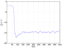
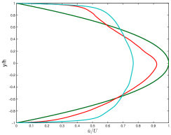
Figure 5.2: Similar to Figure 5.1 but using a boundary condition that fixes the mass flux.

$Re$	$Re_{\tau}$	$\Lambda_{x}$	$\Lambda_{z}$	$L$	$M$	$N$	$\Delta x^{+}$/$\Delta y_{c}^{+}$/$\Delta z^{+}$	$UT_{1}/h$	$UT_{2}/h$	$U\Delta t/h$
$4000$	$171.4$	$2$	$2/3$	$320$	$128$	$128$	$6.7$/$4.2$/$5.6$	$1125$	$300$	$.005$
$10^{4}$	$379.9$	$1$	$1/2$	$320$	$256$	$256$	$7.4$/$4.6$/$4.6$	$580$	$120$	$.002$

Table 1: Parameters of turbulence simulations used for numerical validation. The $\Delta x^{+}/\Delta y_{c}^{+}/\Delta z^{+}$ column gives the grid resolution in wall units, with $\Delta y_{c}^{+}$ being the distance between grid points along $y$ near the center of the channel. The initialization time used to eliminate transients $T_{1}$, the time over statistics is accumulated $T_{2}$, and the time step $\Delta t$ are non-dimensionalized using the centerline speed of the laminar solution $U$ and the channel half-width $h$.

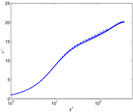
(a)

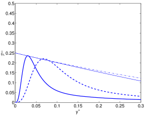
(b)

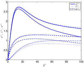
(c)

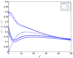
(d)

Figure 5.3: Statistics for the two cases detailed in Table 1. In all the figures, the horizontal axis is $y^{+}$, which denotes the distance from the wall in frictional units. In plots (a) and (b), the dashed lines are for $Re_{\tau}=171$, which is the first row in the table, and the solid line is for the other row with $Re_{\tau}=380$. The data in these plots is compared to classical simulations as well as existing theory in the text. Data from the $Re_{\tau}=392$ simulation by Moser, Kim and Mansour [21] is marked using $+$.

The two test cases used for numerical validation are detailed in Table 1. The two cases are close to but not exactly the same as two of the cases reported in the simulations of Moser et al. [21]. The first test case has $Re_{\tau}=171$ against $Re_{\tau}=180$ in [21]. The second test case has $Re_{\tau}=380$ against $Re_{\tau}=392$ in [21].

The plots in Figure 5.3 may be compared with the plots of Moser et al. [21]. Figure 5.3 (a) shows the mean streamwise velocity as a function of the distance from the wall. This curve is usually fitted using the famous log-law of the wall. Moser et al. discuss power law fits as well. The plot for $Re_{\tau}=380$ is quite close to the plot for $Re_{\tau}=392$ given in [21]. The plot for $Re_{\tau}=171$ shows a pronounced low Reynolds number effect. However, the low Reynolds number effect is much less pronounced in our test than in the $Re_{\tau}=180$ test in [21]. This could be either because of the superior resolution in our test or because of the much longer time integration used to eliminated transients.

Figure 5.3 (b) shows the turbulence energy production as a function of the distance from the wall. The straight lines in the figure are theoretical curves for the peak (solid line) and the envelope (dashed line) derived by Laadhari [15]. Both test cases are in excellent agreement with Laadhari’s theory and simulations.

Figure 5.3 (c) and (d) show turbulence intensities and rms vorticity profiles, respectively. The plots for $Re_{\tau}=380$ are in good agreement with plots for $Re_{\tau}=392$ reported in [21]. There is a noticeable discrepancy in the rms plots of $\omega_{x}$ between our $Re_{\tau}=171$ test case and the $Re_{\tau}=180$ test case of [21]. This discrepancy is most probably due to the superior resolution of our test case. Close observation of the plots in Figure 5.3 shows that the mean streamwise velocity $\bar{u}$ of the $Re_{\tau}=380$ test case is slightly above that of $Re_{\tau}=392$ benchmark (marked using $+$) while the turbulence intensities as indicated by the rms velocity $u^{\prime}$ are more noticeably lower. The slight differences, especially the later, are probably because of the lower value of the frictional Reynolds number in the test case as against the benchmark. The time interval used to gather statistics is another factor which causes slight variations.

6 Conclusion

Green’s function based methods are known to be advantageous for resolving boundary layers. Since boundary layers become thinner as the Reynolds number increases, it is reasonable to try Green’s function based methods for fully developed turbulence. In this paper, we have worked out a numerical method based on Green’s functions for channel flow and plane Couette flow and demonstrated that it is capable of reproducing turbulence phenomena correctly.

Current methods for turbulent channel flow and plane Couette flow are the result of intensive research spanning more than three decades. The Green’s function approach developed here builds upon that research at many points. Green’s functions have not been shown to work for nonlinear problems of the complexity of fully developed turbulence requiring tens of millions of grid points. Getting the Green’s function approach to work for fully developed turbulence is a task in itself.

In the sequel to this paper, the method will be extended in two different directions. The first direction will use a piecewise Chebyshev grid in the wall-normal direction as well as spectral integration, which amounts to implicit use of Green’s functions. The second direction will use a piecewise Chebyshev grid, explicit Green’s functions as developed in this paper, and carefully derived quadrature rules. Both directions appear capable of challenging or going beyond the current state of the art in turbulence simulations.

7 Acknowledgments

We thank Sergei Chernyshenko and Nikolay Nikitin for helpful discussions. We thank Fabian Waleffe and the referees for many valuable suggestions. This research was partially supported by NSF grants DMS-0715510, DMS-1115277, and SCREMS-1026317.

References

- [1] U.M. Ascher, S.J. Ruuth, and B.T.R. Wetton. Implicit-explicit methods for time-dependent partial differential equations. SIAM Journal on Numerical Analysis, 32:797–823, 1995.
- [2] J.P. Boyd. Chebyshev and Fourier Spectral Methods. Dover, 2001.
- [3] M. Charalambides and F. Waleffe. Gegenbauer tau methods with and without spurious eigenvalues. SIAM J. on Numerical Analysis, 47(1):48–68, 2008.
- [4] E.A. Coddington and N. Levinson. Theory of Ordinary Differential Equations. McGraw-Hill, 1955.
- [5] E.A. Coutsias, T. Hagstrom, and D. Torres. An efficient spectral method for ordinary differential equations with rational function coefficients. Mathematics of Computation, 65(214):611–636, 1996.
- [6] M. Crouzeix. Une méthode multipas implicite-explicite pour l’approximation des équations d’évolution paraboliques. Numerische Mathematik, 35(3):257–276, 1980.
- [7] D. Gottlieb and S.A. Orszag. Numerical Analysis of Spectral Methods: Theory and Applications. Society for Industrial and Applied Mathematics, 1993.
- [8] L. Greengard. Spectral integration and two-point boundary value problems. SIAM Journal on Numerical Analysis, 28:1071–1080, 1991.
- [9] L. Greengard and V. Rokhlin. On the numerical solution of two-point boundary value problems. Communications on Pure and Applied Mathematics, 44(4):419–452, 1991.
- [10] E. Hairer, S.P. Norsett, and G. Wanner. Solving Ordinary Differential Equations I. Springer-Verlag, 2nd edition, 2011.
- [11] S. Hoyas and J. Jiménez. Scaling of the velocity fluctuations in turbulent channels up to . Physics of Fluids, 18:011702, 2006.
- [12] J. Jimenez and P. Moin. The minimal flow unit in near-wall turbulence. Journal of Fluid Mechanics, 225(213-240), 1991.
- [13] J. Kim, P. Moin, and R. Moser. Turbulence statistics in fully developed channel flow at low Reynolds number. Journal of Fluid Mechanics, 177(1):133–166, 1987.
- [14] L. Kleiser and U. Schumann. Treatment of incompressibility and boundary conditions in 3-D numerical spectral simulations of plane channel flows. In 3rd Conference on Numerical Methods in Fluid Mechanics, volume 1, pages 165–173, 1980.
- [15] F. Laadhari. On the evolution of the maximum turbulent kinetic energy production in a channel flow. Physics of Fluids, 14:L65–L68, 2002.
- [16] O. A. Ladyzhenskaya. The Mathematical Theory of Viscous Incompressible Flow, 2nd ed. Gordon and Breach, New York, 1969.
- [17] Y.C. Li and Z. Lin. A resolution of the Sommerfeld paradox. SIAM Journal on Mathematical Analysis, 43:1923, 2011.
- [18] A. Lundbladh, D.S. Henningson, and A.V. Johansson. An efficient spectral integration method for the solution of the Navier-Stokes equations. Technical Report FFA TN, 1992-28, 1992.
- [19] A. Lundbladh, D.S. Henningson, and S.C. Reddy. Threshold amplitudes for transition in channel flows. Transition, Turbulence and Combustion, pages 309–318, 1994.
- [20] P. Moin and J. Kim. On the numerical solution of time-dependent viscous incompressible fluid flows involving solid boundaries. Journal of Computational Physics, 35(3):381–392, 1980.
- [21] R.D. Moser, J. Kim, and N.N. Mansour. Direct numerical simulation of turbulent channel flow up to . Physics of Fluids, 11:943–945, 1999.
- [22] N. Nikitin. Finite-difference method for incompressible Navier–Stokes equations in arbitrary orthogonal curvilinear coordinates. Journal of Computational Physics, 217(2):759–781, 2006.
- [23] N. Nikitin. Third-order-accurate semi-implicit Runge–Kutta scheme for incompressible Navier–Stokes equations. International Journal for Numerical Methods in Fluids, 51(2):221–233, 2006.
- [24] D. Rempfer. On boundary conditions for incompressible Navier-Stokes problems. Applied Mechanics Reviews, 59:107, 2006.
- [25] V. Rokhlin. Solution of acoustic scattering problems by means of second kind integral equations. Wave Motion, 5(3):257–272, 1983.
- [26] V. Rokhlin. Rapid solution of integral equations of classical potential theory. Journal of Computational Physics, 60(2):187–207, 1985.
- [27] P.R. Spalart, R.D. Moser, and M.M. Rogers. Spectral methods for the navier-stokes equations with one infinite and two periodic directions. Journal of Computational Physics, 96:297–324, 1991.
- [28] P. Starr and V. Rokhlin. On the numerical solution of two-point boundary value problems II. Communications on Pure and Applied Mathematics, 47(8):1117–1159, 1994.
- [29] S. Toh and T. Itano. Interaction between a large-scale structure and near-wall structures in channel flow. Journal of Fluid Mechanics, 524:249–262, 2005.
- [30] J.M. Varah. Stability restrictions on second order, three level finite difference schemes for parabolic equations. SIAM Journal on Numerical Analysis, 17:300–309, 1980.
- [31] D. Viswanath. Spectral integration of linear boundary value problems. arxiv.org, 2012.
- [32] F. Waleffe. Homotopy of exact coherent structures in plane shear flows. Physics of Fluids, 15:1517, 2003.
- [33] Y.T. Yang and J.Z. Wu. Channel turbulence with spanwise rotation studied using helical wave decomposition. Journal of Fluid Mechanics, 692:137, 2012.
- [34] A. Zebib. A Chebyshev method for the solution of boundary value problems. Journal of Computational Physics, 53(3):443–455, 1984.