Determining Frequentist Confidence Limits Using a Directed Parameter Space Search

Abstract

We consider the problem of inferring constraints on a high-dimensional parameter space with a computationally expensive likelihood function. We propose a machine learning algorithm that maps out the Frequentist confidence limit on parameter space by intelligently targeting likelihood evaluations so as to quickly and accurately characterize the likelihood surface in both low- and high-likelihood regions. We compare our algorithm to Bayesian credible limits derived by the well-tested Markov Chain Monte Carlo (MCMC) algorithm using both multi-modal toy likelihood functions and the 7-year WMAP cosmic microwave background likelihood function. We find that our algorithm correctly identifies the location, general size, and general shape of high-likelihood regions in parameter space while being more robust against multi-modality than MCMC.

1 Introduction

We consider the following problem. A researcher wants to constrain a theory described by some number $N_{p}$ of tunable parameters, which we will represent by the $N_{p}$-dimensional vector $\vec{\theta}$. The available data measure some function $f$ which is an implicit function of $\vec{\theta}$. The researcher is able to calculate a $\chi^{2}$ value quantifying the fit of a model $f(\vec{\theta})$ to the data and wishes to find a confidence limit defined by some rule, e.g $\chi^{2}\leq\chi^{2}_{\text{lim}}$. This is a general phrasing of a Frequentist confidence limit as discussed in Appendix A. We discuss alternatives for determining $\chi^{2}_{\text{lim}}$ in Section 2.1 below. We will also consider the case that the reseracher wishes to find Bayesian credible limt to some probability $(1-\alpha)\%$.

If the calculation going from $\vec{\theta}\rightarrow\chi^{2}$ is rapid, this problem is trivial. One generates a fine grid of points in the $N_{p}$-dimensional parameter space, evaluates $\chi^{2}$ at each of these points, and defines the confidence limit as only those points which satisfy the rule. Often, however, the calcuation $\vec{\theta}\rightarrow\chi^{2}$ is not rapid, or $N_{p}$ is large enough that such a grid-based method will take a prohibitively long time. In that case, one must make intelligent choices regarding which points in parameter space are actually interesting enough to warrant $\vec{\theta}\rightarrow\chi^{2}$ evaluation.

Markov Chain Monte Carlo (MCMC) methods propose to find the desired limits by drawing random samples from the parameter space which are drawn according to a probability density (the Bayesian posterior) which can be interpreted as the probability that some value of $\vec{\theta}$ represents the true value of $\vec{\theta}$ realized by the physical process underlying the data. With enough of these samples, one can integrate this probability density and find regions which contain some set amount of the total probability. In this case, “credible limits” are phrased as target values for the probability integral $(1-\alpha)\%$, i.e. 68% for “1-$\sigma$” limits, 95% for “2-$\sigma$” limits and so on [Gilks et al. 1996].

We propose an alternative solution, using methods from machine learning (to wit, Gaussian processes, though the algorithm admits many possible drivers; see Section 3) to find the desired confidence limit by directly searching the parameter space of $\vec{\theta}$ for points which lie on the boundary of the desired confidence limit $\chi^{2}\leq\chi^{2}_{\text{lim}}$. We refer to this algorithm as Active Parameter Searching (APS). We present the algorithm in detail in Sections 2 and 3. As it searches, APS uses the knowledge it has already learned about $\vec{\theta}\rightarrow\chi^{2}$ to improve its search according to a metric that rewards the algorithm both for finding points on the confidence limit and for sampling points from previously unexplored regions of parameter space. We find that this behavior makes APS more robust against multi-modal $\chi^{2}$ functions (see Section 4) without sacrificing the speed of convergence associated with traditional MCMC methods (see Section 5). We show that, while APS is designed specifically to yield Frequentist confidence limits (which we define in Appendix A), it is also capable of roughly approximating Bayesian credible limits on the space of $\vec{\theta}$ (see Sections 2.4,4 and 5).

Readers should be aware that, while MCMC can be analytically shown to asymptotically sample the Bayesian posterior, APS is designed to discover Frequentist confidence limits purely through exploration, i.e. there is no a priori motivation behind the APS algorithm. Our only demonstration of APS’s efficacy is empirical. It has done well on the problems we have tested it on, though we have tried to choose those problems such that they are representative of problems likely to be encountered by the community. Readers who require theoretically-motivated results will likely need to resort to a sampling routine like MCMC to derive their final constraints. IN the case of multi-modal likelihood functions, the MultiNest algorithm (Feroz and Hobson 2008, Feroz et al. 2009) has been shown to be effective. We hope to show in Section 4 that, even in these use cases, APS can provide a valuable service by identifying the general regions of parameter space over which the Bayesian posterior needs to be integrated, i.e. by guiding users in the process of setting priors and proposal densities for a sampling algorithm, a problem which has posed significant problems for MCMC in the case of multi-modal likelihood functions.

2 The APS Algorithm

The APS algorithm was originally presented by Bryan (2007) as

• (1A) Generate some initial number $N_{s}$ of randomly-distributed points in parameter space. Find the values of $\chi^{2}$ corresponding to these points.
  

• (2A) Generate some number $N_{c}$ of candidate points. For each of these points, find the $N_{g}$ nearest points already sampled by APS (we use a k-d tree as described in Bentley 1975). Use these nearest neighbor points and their corresponding $\chi^{2}$ values to predict the value of $\chi^{2}$ at each of these points. We will signify this prediction by $\mu$. Calculate some value $\sigma$ quantifying confidence in $\mu$ as a prediction of $\chi^{2}$. Low values of $\sigma$ should correspond to confident predictions.
  

• (3A) Choose the candidate point which maximizes the statistic

  $$S=\sigma-|\mu-\chi^{2}_{\text{lim}}|$$ (1)

  and evaluate $\vec{\theta}\rightarrow\chi^{2}$ at that point. Add this point and its $\chi^{2}$ value to the list of sampled points begun in (1A). Return to (2A) and repeat until convergence.
  

The confidence limit reported by APS is the list of all points found for which $\chi^{2}\leq\chi^{2}_{\text{lim}}$. These points, when plotted in one- or two-dimensional slices of parameter space, ought to sketch out a region which contains the true value of $\vec{\theta}$ with the desired confidence (as defined in Appendix A). This is in contrast to the credible limits of MCMC, which represent an integral over the sampled points containing some fraction of the total posterior probability. We present an alternative interpretation for yielding credible limits from APS in Section 2.4.

The $|\mu-\chi^{2}_{\text{lim}}|$ term in equation (1) provides an incentive for APS to choose points that it believes will lie on the boundary of the confidence limit. The $\sigma$ term provides an incentive for APS to explore unknown regions of parameter space, making the algorithm robust against multimodal $\chi^{2}$ functions.

In the present work, we introduce modifications and expansions to this basic algorithm as described below.

2.1 Determining $\chi^{2}_{\text{lim}}$

As discussed above, APS draws confidence limits by mapping iso-$\chi^{2}$ contours of $\chi^{2}=\chi^{2}_{\text{lim}}$ in parameter space. Thus, the user is presented with the problem of determining an appropriate $\chi^{2}_{\text{lim}}$. APS admits two possible solutions. The user can fiat a definite value of $\chi^{2}_{\text{lim}}$ based on the characteristics of the data at hand, or $\chi^{2}_{\text{lim}}$ can be set adaptively, based on APS’ knowledge of $\vec{\theta}\rightarrow\chi^{2}$.

The first possibility, a user-defined $\chi^{2}_{\text{lim}}$, is based on the theory of Frequentist confidence intervals, which we briefly discuss here and consider in much greater detail in Appendix A. If a data set is comprised of $N_{d}$ Gaussian-distributed data points with a known covariance structure, then

$$\chi^{2}\equiv\sum_{i,j}^{N_{d}}(d_{i}-f_{i}(\vec{\theta}))C^{-1}_{i,j}(d_{j}-f_{j}(\vec{\theta}))$$ (2)

will be distributed according to a $\chi^{2}$-distribution with $N_{d}$ degrees of freedom. This distribution can be integrated to determine the value of $\chi^{2}$ containing $(1-\alpha)\%$ of the total probability. This limiting value will be the user-defined $\chi^{2}_{\text{lim}}$.

If the user does not feel comfortable settig $\chi^{2}_{\text{lim}}$ a priori, APS $\chi^{2}_{\text{lim}}$ can learn $\chi^{2}_{\text{lim}}$ by defining it as $\chi^{2}_{\text{min}}+\Delta\chi^{2}$. Here, $\chi^{2}_{\text{min}}$ is the minimum value of $\chi^{2}$ discovered by APS. $\Delta\chi^{2}$ is set based on the properties of the $N_{p}$-dimensional parameter space being explored. To wit, Wilks (1938) proves that $\Delta\chi^{2}$ for an $N_{p}$-dimensional parameter space will be distributed according to a $\chi^{2}$-distribution with $N_{p}$ degrees of freedom. One can perform the same integral discussed above and set $\Delta\chi^{2}$ to that value which encloses the desired confidence limit. This is the well-known Likelihood Ratio Test [Neyman and Pearson 1933]. In this case, the user is relying on APS to eventually find the true $\chi^{2}_{\text{min}}$ of the likelihood surface being explored. Section 2.2.3 below outlines an additional means of search by which our expanded APS is capable of efficiently locating $\chi^{2}_{\text{lim}}$.

2.2 Modified search algorithms

Bryan et al. (2007) show that the APS search algorithm as presented in steps (1A-3A) is robust against multi-modal likelihood functions, using it to identify a disjoint region of high likelihood in cosmological parameter space as constrained by the 1-year WMAP CMB anisotropy power spectrum. This is the principal advantage to selecting points for evaluation according to the statistic (1). Unfortunately, it is possible that the focus on exploring unknown regions of parameter space might slow down convergence in the case of uni-modal likelihood functions. Therefore, we augment steps (1A-3A) with the following modified search algorithms to ensure that APS adequately characterizes known regions of high likelihood while simultaneously searching for new regions to explore.

These modified searches will require APS to keep track of information it learns about the $\vec{\theta}\rightarrow\chi^{2}$ fuction as it searches. To facilitate this discussion, we introduce the following notation. Symbols denoted with $\vec{x}$ represent points in parameter space. Variables denoted with $\{\hat{X}\}$ denote sets of points in parameter space. Variables denoted $\{X\}$ are sets of numbers stored by APS.

We are greatly indebted to Eric Linder of the Lawrence Berkeley National Laboratory who first suggested to us the modifications described below in sections 2.2.1 and 2.2.3.

2.2.1 Characterization of known low-$\chi^{2}$ regions

As it searches, APS will keep track of a list of all of the discovered points which are believed to be local minima of $\chi^{2}$ (how it finds these will be described below in Section 2.2.3). These points will be stored in the set $\{\hat{\Gamma}\}$. After each cycle of the main algorithm (steps 1A-3A above), our version of APS attempts “focused searches” about the points in $\{\hat{\Gamma}\}$.

For each point $\vec{M}$ in $\{\hat{\Gamma}\}$, APS performs the following:

• (1B) If fewer than $N_{p}$ focused searches have been proposed about $\vec{M}$, randomly choose a point from a small sphere surrounding $\vec{M}$ in parameter space and evaluate $\chi^{2}$ at that point.
  

• (2B) If the point does not satisfy $\chi^{2}=\chi^{2}_{\text{lim}}$ (which is highly probable), use bisection along the line connecting the proposed point to $\vec{M}$ to find a point which does satisfy $\chi^{2}=\chi^{2}_{\text{lim}}$, i.e. find a point on that line for which $\chi^{2}<\chi^{2}_{\text{lim}}$ – often $\vec{M}$ itself – and a point along that line for which $\chi^{2}>\chi^{2}_{\text{lim}}$ and iteratively step half the distance between them until arriving at the desired $\chi^{2}_{\text{lim}}$ [James 1972]. The points discovered in this way  with $\chi^{2}=\chi^{2}_{\text{lim}}$ are stored in the set $\{\hat{B}(\vec{M})\}$ of “boundary points” about $\vec{M}$ (each $\vec{M}$ in $\{\hat{\Gamma}\}$ will have its own set $\{\hat{B}(\vec{M})\}$).
  

• (3B) If $N_{p}$ boundary points have been found for $\vec{M}$, skip steps (1B) and (2B). Instead, examine the points in $\{\hat{B}(\vec{M})\}$ and identify the points corresponding to both the maximum and minimum values of each parameter $\theta_{i}$. These points will be referred to as $\{\hat{B}_{\text{MaxMin}}(\vec{M})\}$. There will be $2\times N_{p}$ points in $\{\hat{B}_{\text{MaxMin}}(\vec{M})\}$, one for the maximum and one for the minimum in each of our $N_{p}$ parameters.
  

• (4B) For each point $\vec{b}$ in $\{\hat{B}_{\text{MaxMin}}(\vec{M})\}$, propose some number $N_{v}$ of new points (we have chosen $N_{v}=20$ for the sake of speed) $\vec{v}=\vec{b}+\vec{\epsilon}$ where $\vec{\epsilon}$ is a random, small vector in parameter space constrained to be perpendicular to $\vec{b}-\vec{M}$. There will now be $2\times N_{p}\times N_{v}$ points $\vec{v}$ ($N_{v}$ such points for each of the $2\times N_{p}$ extremal boundary points in $\{\hat{B}_{\text{MaxMin}}(\vec{M})\}$).
  

• (5B) At each point $\vec{v}$ above, find the $N_{g}$ nearest neighbor points as in step (2A) above and evaluate equation (1). Find the point $\vec{v}$ which maximizes $S$ and evaluate $\vec{\theta}\rightarrow\chi^{2}$ at that point. If $\chi^{2}\neq\chi^{2}_{\text{lim}}$, use bisection to find a new boundary point. Store the resulting $\chi^{2}=\chi^{2}_{\text{lim}}$ point in $\{\hat{B}(\vec{M})\}$

The modification suggested in section 2.2.1 is designed to explore $\chi^{2}=\chi^{2}_{\text{lim}}$ surface by starting from its extreme corners and stepping perpendicularly to its “radii” (the vector $\vec{b}-\vec{M}$ would be a radius if $\chi^{2}=\chi^{2}_{\text{lim}}$ described a sphere), with the hope of being able to extend the bounds of $\{\hat{B}_{\text{MaxMin}}(\vec{M})\}$. In this way, our extended APS attempts to plumb the full Frequentist confidence limit $\chi^{2}\leq\chi^{2}_{\text{lim}}$ as rapidly as possible. However, we do not want this to come at the expense of the wide-ranging exploration of steps (1A-3A). Our version of APS alternates between performing steps (1A-3A) and steps (1B-5B). If there are $N_{m}$ distinct known local minima in $\{\hat{\Gamma}\}$, our algoritm will perform $N_{m}$ iterations of steps (1A-3A), and then perform steps (1B-5B) once for each $\vec{M}$ in $\{\hat{\Gamma}\}$.

2.2.2 Extension of the $\chi^{2}=\chi^{2}_{\text{lim}}$ contour

It is, however, also possible that the $S$-maximization in steps (1A-3A) could learn something about the shape of the $\chi^{2}=\chi^{2}_{\text{lim}}$ contour, even if it does not place points directly on that contour. To explore that possibility, our extended APS performs the following modified search after each iteration of steps (1A-3A).

• (1C) For each point $\vec{M}$ in $\{\hat{\Gamma}\}$, store, in addition to the boundary points $\{\hat{B}(\vec{M})\}$, the projection of those boundary points onto a unit sphere in parameter space, i.e. for each point $\vec{b}$ in $\{\hat{B}(\vec{M})\}$, draw a line connecting $\vec{b}$ with $\vec{M}$ and keep track of where a unit sphere centered on $\vec{M}$ intersects that line. Call this set of projections $\{\hat{U}\}$.
  

• (2C) Call the point for which $\chi^{2}$ has been evaluated in step (3A) $\vec{P}$. Find the point $\vec{M}$ in $\{\hat{\Gamma}\}$ that is nearest to $\vec{P}$ in parameter space.
  

• (3C) Find the projection of $\vec{P}$ onto the unit sphere surrounding $\vec{M}$. Call this projected point $\vec{p}$. Find the point $\vec{u}$ in $\{\hat{U}\}$ that is nearest to $\vec{p}$. Record the parameter space distance between $\vec{u}$ and $\vec{p}$. Add this distance to the set $\{D\}$ ($\{D\}$ will be a running list of the $\vec{u}-\vec{p}$ distance for all points $\vec{P}$ found by steps 1A-3A, regardless of which point in $\vec{M}$ they are nearest).
  

• (4C) If the $\vec{p}-\vec{u}$ distance is greater than the 2/3 quantile of $\{D\}$, then perform bisection between $\vec{M}$ and the point evaluated in step (3A). Add the resulting $\chi^{2}=\chi^{2}_{\text{lim}}$ point to $\{\hat{B}(\vec{M})\}$.

Step (4C) ensures that, if the point $\vec{P}$ is in a novel direction from $\vec{M}$, APS will find a point on the $\chi^{2}=\chi^{2}_{\text{lim}}$ contour in that direction. Because $\vec{P}$ was chosen by maximizing equation (1), we assume that there was something “interesting” about that direction from $\vec{M}$ (perhaps a sharp corner or distended extension of the $\chi^{2}=\chi^{2}_{\text{lim}}$ contour). In this way, our extended APS will attempt to cover the surface of $\chi^{2}=\chi^{2}_{\text{lim}}$ in the most informative way possible.

Because we expect the unit spheres surrounding the points $\vec{M}$ to become more densely populated as the algorithm runs, we periodically delete the list $\{D\}$ so that new directions away from $\vec{M}$ can still be explored.

2.2.3 Function minimization

The penultimate modification to the original APS algorithm which we propose in this work is to utilize function minimization to identify local minima in $\chi^{2}$. One of the principal drawbacks of the algorithm presented in steps (1A-3A) is that it makes no account of “near misses.” If step (3A) finds that $\chi^{2}$ is lower than average but still greater than $\chi^{2}_{\text{lim}}$, the original APS algorithm does nothing with that information. We have tried to improve upon that with our incorporation of bisection in sections 2.2.1 and 2.2.2 above. An additional innovation is to allow APS to use points with

$$\chi^{2}_{\text{lim}} \leq \chi^{2}\leq\chi^{2}_{\text{threshold}}$$ (3)

$$\chi_{\text{threshold}} \equiv \chi^{2}_{\text{min}}+G\times(\chi^{2}_{1/10}-\chi^{2}_{\text{min}})$$ (4)

to seed a simplex function minimizer as developed by Nelder and Mead (1965). Here, $G$ is a user-set parameter, $\chi^{2}_{\text{min}}$ is the minimum discovered $\chi^{2}$ value and $\chi^{2}_{1/10}$ is the 1/10 quantile of the $\chi^{2}$ values discovered by steps (1A-3A) (not those discovered by any of the modifications discussed in sections 2.2.1, 2.2.2 or 2.2.3).

Because the Nelder-Mead simplex minimizer can be very time intensive, we balance our algorithm by keeping track of how many times $\vec{\theta}\rightarrow\chi^{2}$ is called by the different searches and demanding that the number of $\chi^{2}$ evaluations devoted to all other variants of search (i.e. steps (1A-3A), (1B-5B), and (1C-4C)) equal the number of $\chi^{2}$ evaluations devoted to the simplex minimizer before a new simplex minimization can occur.

If the simplex minimizer converges to a point such that $\chi^{2}<\chi^{2}_{\text{lim}}$, our extended APS determines whether or not it has found a new local minimum to be added to $\{\hat{\Gamma}\}$ by comparing the end point $\vec{y}$ of the minimization to each of the points already in $\{\hat{\Gamma}\}$. For each $\vec{M}$ in $\{\hat{\Gamma}\}$, APS calculates the mid-point

$$\vec{m}(\vec{M})=0.5\times\left(\vec{y}+\vec{M}\right)$$ (5)

If, for all $\vec{M}$, $\chi^{2}$ at $\vec{m}(\vec{M})$ is greater than $\chi^{2}_{\text{lim}}$, then it is deemed that $\vec{y}$ is a new local minimum and is added to $\{\hat{\Gamma}\}$. If not, $\vec{y}$ is assumed to be a part of the one of the previously identified loci of low $\chi^{2}$ and it is not added to $\{\hat{\Gamma}\}$. Regardless of whether or not $\vec{y}$ passes the test in equation (5), $\vec{y}$ is added to the set $\{\hat{Y}\}$ of all simplex end points discovered by APS.

As a further guard against excessive simplex searching, all points $\vec{w}$ that pass the test in equation (3) are further required to satisfy the condition

$$\chi^{2}(\vec{z}) > \chi^{2}(\vec{w})-0.25\times\left(\chi^{2}(\vec{w})-\chi^{2}(\vec{y})\right)$$ (6)

$$\vec{z} \equiv 0.5\times\left(\vec{w}+\vec{y}\right)$$ (7)

$$\vec{y} \in \{\hat{Y}\}$$ (8)

before they are allowed to seed a new simplex search. In this way, our extended APS avoids seeding simplex searches with points that are inside of already known regions of low $\chi^{2}$.

2.2.4 Simplex-driven APS search

Having introduced the concept of the Nelder-Mead (1965) simplex search in Section 2.2.3 above, we additionally use this tool to improve upon the original APS search algorith, steps (1A)-(3A). Broadly speaking, the purpose of the original APS algorithm is to identify the point which maximizes the $S$ statistic in equation (1) and evaluate $\vec{\theta}\rightarrow\chi^{2}$ at that point. As more points are sampled, $S$ will, presumably, come to be maximized at points that are near the $\chi^{2}=\chi^{2}_{\text{lim}}$ contour, but far from other sampled points, so APS will efficiently explore the parameter space. Steps (1A)-(3A) approximately achieve this end by proposing a random sample of candidate points and evaluating $\vec{\theta}\rightarrow\chi^{2}$ at the point which maximizes $S$ within that sample. We use the Nelder-Mead (1965) simplex to replace this process as follows:

• (1Ã) Perform step (1A) as above.
  

• (2Ã) Generate $N_{p}+1$ randomly chosen points $\{\hat{R}\}$ in parameter space. For each point $\vec{r}$ in $\{\hat{R}\}$, use equation (1) as in steps (2A-3A) above to calculate $S$. This set of $S$ values will be called $\{S\}$.
  

• (3Ã) Use $\{\hat{R}\}$ and $\{S\}$ as the seed for a Nelder-Mead (1965) simplex search. At each subsequent point sampled by this search, calculate $S$ as above. Run this simplex until $S$ converges to a local maximum.
  

• (4Ã) Evaluate $\vec{\theta}\rightarrow\chi^{2}$ at the point which maximized $S$. Add this point to the list of points sampled by APS. Return to step (2Ã). Repeat until convergence.

By choosing the maximum $S$ point based on a simplex search rather than a finite random sample, we hope to find a true local maximum in $S$, rather than just the maximum relative to the limited number of sample points chosen. Steps (1Ã)-(4Ã) replace steps (1A)-(3A) in our expanded APS algorithm.

2.3 Code implementing APS

We make code implementing our extended APS for an arbitrary $\vec{\theta}\rightarrow\chi^{2}$ function available at https://github.com/uwssg/APS/. The code is written in C++. It is designed for users to use with any $\vec{\theta}\rightarrow\chi^{2}$ function. Users need only to write a sub-class of the chisquared class defined in chisq.h and chisq.cpp which evaluates their desired $\vec{\theta}\rightarrow\chi^{2}$ and pass an instantiation of this sub-class to an instantiation of the aps class defined in aps.h and aps.cpp. It is this aps class which does the work of performing the searches described above. The user should not need to modify this class (though she is certainly welcome to).

Our aps class provides the option for several user-specified parameters. We list them below along with the C++ methods (belonging to the class aps) used to set them.

• The parameter $G$ from equation (4) above can be set using the method aps.set_grat
  

• $\chi^{2}_{\text{lim}}$ can be manually set using the method aps.set_target
  

• $\Delta\chi^{2}$ can be set in the constructor for the class aps.
  

• The number $N_{g}$ of nearest neighbors used in steps (2Ã)-(3Ã) can be set in the constructor for the class aps
  

• The minimum and maximum bounds in parameter space can be set using the method aps.set_max and aps.set_min. These bounds will constrain the range of points sampled in step (2Ã)-(3Ã). They will not contrain searches performed with bisection or the simplex minimizer.
  

• If there is a characteristic length scale associated with a parameter, this can be set using the method aps.set_characteristic_length. This length scale will be used to normalize all distances in parameter space. If it is not set, it will default to the difference between the maximum and minimum values set by aps.set_max and aps.set_min. Setting a characteristic length scale will principally affect what points are considered nearest neighbors for the purposes of steps (2Ã)-(3Ã). If the characteristic length scale of a parameter is large, that parameter will be down-weighted when calculating the parameter-space distance between two points. If the characteristic length scale of a parameter is small, that parameter will be up-weighted in length calculations.

More complete documentation is made available with the source code.

2.4 Interpreting APS outputs

Originally, APS was conceived as a way to draw Frequentist confidence limits $\chi^{2}\leq\chi^{2}_{\text{lim}}$. This is by far the most direct way to interpret APS outputs: a list of points is given with corresponding values of $\chi^{2}$. All of the points with $\chi^{2}\leq\chi^{2}_{\text{lim}}$ are taken to cover the desired confidence limit. There is, however, also a way to use the outputs from APS to draw an approximate Bayesian credible limit.

As discussed in the introduction, Bayesian parameter constraints assume that there is some probability distribution (“the posterior”) over $\vec{\theta}$. $(1-\alpha)\%$ credible limits are drawn by integrating over this probability distribution and selecting that region which contains $(1-\alpha)\%$ of the total probability. This integral can be very time-consuming if the dimensionality of $\vec{\theta}$ is large. Markov Chain Monte Carlo methods overcome this difficulty by randomly drawing samples from the posterior and assuming that, if enough samples are drawn, the distribution of those samples will be sufficient to reconstruct the attributes of the full posterior probability density.

APS outputs cannot be used this way, since APS does not select its points probabilisticaly, but in an attempt to recreate the behavior of the $\vec{\theta}\rightarrow\chi^{2}$ function in interesting regions of parameter space. We can still, however, use these points to approximate the integral over the posterior probability density. The algorithm we propose is as follows. The total set of points sampled by APS will be referred to below as $\{\hat{A}\}$.

For each $\vec{a}$ in $\{\hat{A}\}$:

• (1D) Initialize two vectors $\vec{a}_{\text{max}}$ and $\vec{a}_{\text{min}}$. Set all of the values in these vectors to some nonsense number.

• (2D) Select the $3N_{p}+1$ nearest neighbor points to $\vec{a}$ from $\{\hat{A}\}$ (this will obviously include $\vec{a}$ itself, which can be discarded). Call this set of nearest neighbors $\{\hat{N}\}$.
  

• (3D) For each point $\vec{n}$ in $\{\hat{N}\}$, calculate the vector $\vec{\delta}$ such that $\delta_{i}=|n_{i}-a_{i}|$ (here the vertical bars denote the absolute value). For each component $\delta_{i}$ of $\vec{\delta}$, starting with the largest and working towards the smallest:
  

  • (3Da) If $n_{i}>a_{i}$ and $a_{\text{max},i}$ has not been set, set $a_{\text{max},i}=n_{i}$.
    

  • (3Db) If $n_{i}<a_{i}$ and $a_{\text{min},i}$ has not been set, set $a_{\text{min},i}=n_{i}$.
    

  • (3Dc) If both $a_{\text{max,i}}$ and $a_{\text{min,i}}$ have already been set, move on to the next largest $\delta_{i}$ and repeat at step (3Da).
    

• (4D) $\vec{a}_{\text{max}}$ and $\vec{a}_{\text{min}}$ should now describe an asymmetric, rectangular hyperbox about $\vec{a}$. To symmetrize it, step through all $N_{p}$ dimensions and reset either $a_{\text{max},i}$ or $a_{\text{min},i}$ so that $d_{\text{min}}=a_{i}-a_{\text{min},i}$ and $d_{\text{max}}=a_{\text{max},i}-a_{i}$ are equal to the minimum of $\{d_{\text{max}},d_{\text{min}}\}$ from the asymmetric hyperbox. Return to step (1D) and repeat for the next $\vec{a}$.

At this point, each $\vec{a}$ in $\{\hat{A}\}$ should have a corresponding symmetric hyperbox surrounding it described by the corresponding $\vec{a}_{\text{max}}(\vec{a})$ and $\vec{a}_{\text{min}}(\vec{a})$. To integrate the posterior probability density, we will assume that all of the parameter space points in each hyperbox correspond to $\chi^{2}=\chi^{2}(\vec{a})$, i.e. the $\chi^{2}$ discovered by APS for the point at the center of the hyperbox is the $\chi^{2}$ value for all of the points inside the hyperbox. The posterior probability associated with each box is then

$$P(\vec{a}) = \frac{V(\vec{a})}{P_{\text{tot}}}\times\exp\left[-\chi^{2}(\vec{a})/2\right]$$ (9)

$$P_{\text{tot}} \equiv \sum_{\vec{a}}V(\vec{a})\times\exp\left[-\chi^{2}(\vec{a})/2\right]$$ (10)

where $V(\vec{a})$ is the hypervolume of the hyperbox surrounding $\vec{a}$. To plot the $(1-\alpha)\%$ credible limit, one need only plot the points in hyperspace that enclose the lowest-$\chi^{2}$ hyperboxes containing $(1-\alpha)\%$ of the total probability. We test this algorithm on a function with an exactly known credible limit in Section 4 (see Figures 5-7) and on a real, physical dataset in Section 5 (see Figure 14). In Section 4, we find that our results agree with the known credible limit. In Section 5 we find that APS correctly identifies the region and general shape of the Bayesian credible limits, however, with significant noise. The Bayesian credible limits found by APS are systematically larger than the Bayesian credible limits found by MCMC. This motivates our claim in the introduction that APS may be principally useful for identifying regions of high posterior density on largely unknown likelihood functions, allowing users to more shrewdly set priors for sampling algorithms like MCMC.

The functionality described by this section is provided by the classes defined in the source code file aps_extractor.cpp in our software package.

3 Gaussian processes

Steps (2Ã)-(3Ã) of APS requires that a prediction $\mu$ be made regarding the value of $\chi^{2}$ at points as yet unsampled by the algorithm. An uncertainty $\sigma$ must also be assigned to this prediction. APS writ large is agnostic regarding the method used to find $\mu$ and $\sigma$. We choose to use a Gaussian process.

Gaussian processes take noisy, sparse, measurements of an unknown function (in our case, $\vec{\theta}\rightarrow\chi^{2}$ at the points in parameter space already sampled by APS) and use them to make inferences about unmeasured values of the function by assuming that the function is a random process. Gaussian processes have already found use in physics and astronomy constructing non-parametric models of the cosmic expansion [Shafieloo et al. 2012], interpolating the point spread function across astronomical images [Bergé et al. 2012], and interpolating models of the non-linear matter power spectrum from N-body simulations [Habib et al. 2007]. They are useful in the current context because, not only do they give robust predictions $\mu$ for the unmeasured values of the function being modeled, but they also provide well-motivated prediction uncertainties $\sigma$, a requirement of equation (1). We present below an introduction to the formalism of Gaussian processes drawn heavily from Chapter 2 and Appendix A of [Rasmussen and Williams 2006].

Gaussian processes use the sampled data $\{\vec{\theta}^{(i)},\chi^{2,(i)}\}$, where $i$ indexes over all of the sampled points, to predict $\mu=\chi^{2,(q)}$ at the unknown point $\vec{\theta}^{(q)}$ by assuming that the function $\vec{\theta}\rightarrow\chi^{2}$ represents a sample drawn from a random process distributed across parameter space. At each point in parameter space, $\chi^{2}$ is assumed to be distributed according to a normal distribution with mean $\bar{\chi}^{2}$ and variance dictated by the “covariogram” $C_{ij}(\vec{\theta}^{(i)},\vec{\theta}^{(j)})$. If we have $N_{g}$ measurements of $\chi^{2}$ (recall from steps (2Ã-3Ã) above that, for each point where we must predict the value of $\chi^{2}$, we are only using the $N_{g}$ nearest neighbor sampling points as data), then we assume they are distributed according to

$$P(\vec{\chi}^{2})=\frac{\exp\bigg{[}-\frac{1}{2}K^{-1}\sum_{i,j}^{N_{g}}(\chi^{2,(i)}-\bar{\chi}^{2})C^{-1}_{ij}(\chi^{2,(j)}-\bar{\chi}^{2})\bigg{]}}{\sqrt{2\pi}^{N_{g}}\text{det}|KC|^{N_{g}/2}}$$ (11)

$C_{ij}$ is a function assumed by the user encoding how variations in $\chi^{2}$ at one point in parameter space affect variations in $\chi^{2}$ at other points in parameter space. $K$ is a parameter controlling the normalization of $C_{ij}$. The diagonal elements $C_{ii}=1+\sigma^{2}_{ii}$ where $\sigma^{2}_{ii}$ is the intrinsic variance in the value of $\chi^{2}$ at a single point $\vec{\theta}^{(i)}$. Rasmussen and Williams (2006) treat the special case $\bar{\chi}^{2}=0$ and find (see their equations 2.19, 2.25 and 2.26)

$$\mu = \sum_{i,j}^{N_{g}}C_{qi}C^{-1}_{ij}\chi^{2,(j)}$$

$$\sigma^{2} = K\times\left(C_{qq}-\sum_{i,j}^{N_{g}}C_{qi}C^{-1}_{ij}C_{jq}\right)$$ (12)

where the sums over $i$ and $j$ are sums over the sampled points in parameter space. $C_{iq}$ relates the sampled point $i$ to the candidate point $q$. We do not wish to assume that the mean value of $\chi^{2}$ is zero everywhere. Therefore, we modify the equation for $\mu$ to give

$$\mu=\bar{\chi}^{2}+\sum_{i,j}^{N_{g}}C_{qi}C^{-1}_{ij}(\chi^{2,(j)}-\bar{\chi}^{2})$$ (13)

where $\bar{\chi}^{2}$ is the algebraic mean of the sampled $\chi^{2,(i)}$. Note the similarity to a multi-dimensional Taylor series expansion with the covariance matrix playing the role of the derivatives. Equation (12) differs from equation (6) in [Bryan et al. 2007] because they used the semivariance

$$\gamma_{ij}=\text{var}[\chi^{2}(\vec{\theta}^{(i)})-\chi^{2}(\vec{\theta}^{(j)})]$$

in place of the covariance $C_{ij}$. In practice, the two assumptions result in equivalently valid $\mu$ and $\sigma$.

The form of the covariogram $C_{ij}(\vec{\theta}^{(i)},\vec{\theta}^{(j)})$ must be assumed. One possibility, taken from equation 4.9 of Rasmussen and Williams (2006) is

$$C_{ij}=\exp\left[-\frac{1}{2}D^{2}_{ij}\right]$$ (14)

where $D_{ij}$ is the normalized distance in parameter space between the points $\vec{\theta}^{(i)}$ and $\vec{\theta}^{(j)}$.

$$D^{2}_{ij}\equiv\sum_{n}^{N_{p}}\left(\frac{\theta^{(i)}_{n}-\theta^{(j)}_{n}}{\ell_{n}\times(\text{max}_{n}-\text{min}_{n})}\right)^{2}$$ (15)

where $\text{max}_{n}-\text{min}_{n}$ is the difference between the maximum and minimum values of the $n$th parameter taken from the $N_{g}$ points used to seed the Gaussian process and $\ell_{n}$ is a “hyper-parameter” associated with the $n$th parameter. We discuss the normalization paramter $K$ below in section 3.1. We discuss the setting of hyper-parameters in section 3.2. The exponential form of $C_{ij}$ quantifies the assumption that distant points should not be very correlated.

Another possibility (equation 4.29 of Rasmussen and Williams) is

$$C_{ij}=\phantom{\sin\bigg{[}\frac{2(\sigma_{0}+\tilde{\vec{\theta}}^{(i)}\cdot\tilde{\vec{\theta}}^{(j)})}{\sqrt{(1+2(\sigma_{1}+\tilde{\vec{\theta}}^{(i)}\cdot\tilde{\vec{\theta}}^{(i)}))(1+2(\sigma_{1}+\tilde{\vec{\theta}}^{(j)}\cdot\tilde{\vec{\theta}}^{(j)}))}}\bigg{]}}$$ (16)

$$\frac{2}{\pi}\sin^{-1}\bigg{[}\frac{2(\sigma_{0}+\tilde{\vec{\theta}}^{(i)}\cdot\tilde{\vec{\theta}}^{(j)})}{\sqrt{(1+2(\sigma_{1}+\tilde{\vec{\theta}}^{(i)}\cdot\tilde{\vec{\theta}}^{(i)}))(1+2(\sigma_{1}+\tilde{\vec{\theta}}^{(j)}\cdot\tilde{\vec{\theta}}^{(j)}))}}\bigg{]}$$

corresponding to the covariance function of a neural network with a single hidden layer. In this function $\tilde{\vec{\theta}}$ is the vector of parameters $\vec{\theta}$ recentered and renormalized relative to the span $(\text{max}_{n}-\text{min}_{n})$ in each dimension. $\sigma_{0}$ and $\sigma_{1}$ are hyper-parameters. In Section 5, we test APS using both covarigorams (14) and (16) and find no appreciable difference in the resulting parameter constraints.

3.1 Normalizing the covariogram

The normalization constant $K$ in equation (11) – known as the “Kriging parameter” for the geophysicist who pioneered the overall method – also must be assumed. Determining the value of $K$ is somewhat problematic because, examining equation (13), one sees that the factors of $K$ and $K^{-1}$ cancel out of the prediction $\mu$, so that the assumed value of $K$ has no effect on the accuracy of the prediction. If the opposite had been true, one could heuristically set $K$ to maximize the accuracy of $\mu$. Instead, we set $K$ to the value that maximizes the likelihood of the input data, i.e. the $N_{g}$ nearest neighbors in parameter space used to perform the Gaussian process inference.

Recall from equation (11) that we are treating our input data as though they were samples drawn from a probability distribution. To maximize the probability of the observed data (i.e. maximizing the value of $P(\vec{\chi}^{2})$ in equation 11) we must set $K$ equal to

$$K=\frac{\sum_{i,j}^{N_{g}}(\chi^{2,(i)}-\bar{\chi}^{2})C^{-1}_{ij}(\chi^{2,(j)}-\bar{\chi}^{2})}{N_{g}}$$ (17)

We adopt this assumption throughout this work.

Figure 1 applies the Gaussian process of equations (12), (13), and (17) with covariogram (14) to a toy one-dimensional function. Inspection shows many desirable behaviors in $\mu$ and $\sigma$. As $\theta^{(q)}$ approaches the sampled points $\theta^{(i)}$, $\mu$ approaches $\chi^{2,(i)}$ and $\sigma$ approaches zero. Closer to a sampled point, the Gaussian process knows more about the true behavior of the function. Far from the $\theta^{(i)}$, $\sigma$ is larger, and the $S$ statistic in equation (1) will induce the APS algorithm to examine the true value of $\chi^{2}$.

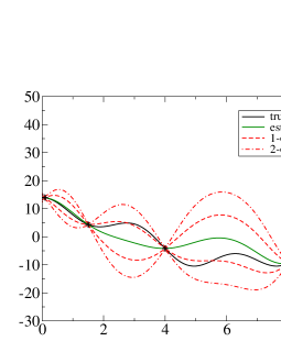
Figure 1: A one-dimensional example of prediction using Gaussian processes. The black curve is the function being considered. The crosses are the points at which it has been sampled. The green curve is the resulting prediction and the red curves represent the 1- and 2-$\sigma$ uncertainty bounds. We set $K$ according to equation (17) wth $N_{g}=5$ for the 5 sampled points.

3.2 Setting hyper-parameters

The covariograms $C_{ij}$ presented above in equations (14) and (16) (indeed, any covariogram) each contain arbitrary hyper-parameters whose values can be set to fine-tune the Gaussian process model ($\ell_{n}$ in equation 14 and $\{\sigma_{0},\sigma_{1}\}$ in equation 16). In order to set the hyper-parameters used in the APS Gaussian process, we randomly select a set $\{\hat{V}\}$ of up to 3000 points from those already sampled by APS and use these to construct the error function $E(\vec{h})$ where $\vec{h}$ is a vector specifying the hyper-parameters required by the chosen $C_{ij}$. $E$ is defined as

$$E(\vec{h})=\sum_{\vec{v}\in\{\hat{V}\}}\left(\mu(\vec{v},\vec{h})-\chi^{2}(\vec{v})\right)^{2}$$ (18)

where $\mu(\vec{v},\vec{h})$ is calculated according to equation 13 using hyper-parameters $\vec{h}$ (and ignoring $\vec{v}$ as its own nearest neighbor) and $\chi^{2}(\vec{v})$ is already known, since $\vec{v}$ has been chosen from the points previously sampled by APS. If $\vec{h}$ has more than two dimensions, we minimize $E$ on $\vec{h}$-space using the simplex minimizer of Nelder and Mead (1965). Otherwise, we do a simple grid search for the value of $\vec{h}$ which minimizes $E$. This optimal value of $\vec{h}$ is used to set the hyper-parameters for our Gaussian process model.

As APS samples more points in parameter space, we expect it to learn more about the $\vec{\theta}\rightarrow\chi^{2}$ function and thus be capable of a more accurate Gaussian process, so we allow it to periodically reset the hyper-parameters $\vec{h}$. However, minimizing $E$ can be a very time-consuming process, so we have APS keep track of the amount of time elapsed since the algorithm began. We divide this value by the number of calls made to the $\vec{\theta}\rightarrow\chi^{2}$ function to give the average total time spent per call to $\vec{\theta}\rightarrow\chi^{2}$ with all of the overhead imposed by APS included. We compare this average with the average amount of time spent on just $\vec{\theta}\rightarrow\chi^{2}$, without any of the overhead imposed by APS. APS is only allowed to reset its hyper-parameters if the difference between these two times is less than 0.1 second per call to $\vec{\theta}\rightarrow\chi^{2}$ (of course, we do require that APS optimize its hyper parameters at least once, so that we can have confidence in our Gaussian process model).

4 A Toy Example

We will now test the ability of APS to learn the confidence limits of an artificial $\chi^{2}$ function and compare it to that of MCMC driven by the traditional Metropolis-Hastings algorithm [Gilks et al. 1996, Lewis and Bridle 2002].

The algorithm (1A)-(3A) in Section 2 was originally presented and tested against the 1-year data release from the WMAP satellite in Bryan et al. (2007). They found that the algorithm detected a second locus of low $\chi^{2}$ that had gone undetected by previous, MCMC-based analyses of the data. This second fit to the data has disappeared as the signal-to-noise ratio of the data has improved (as we will see in Section 5), therefore, we will use for our test a toy $\chi^{2}$ function with multiple locii of low $\chi^{2}$.

We construct our toy $\chi^{2}$ as a series of low-$\chi^{2}$ ellipses in a 5-dimensional parameter space (we choose a 5-dimensional parameter space because it allows us to reasonably show all of the 2-dimensional sub-spaces in the plots which follow). We consider functions with 2, 3, and 4 discrete minima in $\chi^{2}$. The location of the low-$\chi^{2}$ regions are generated using a pseudo random number generator taken from Marsaglia (2003) with parameters taken from Press et al. (2007). $\chi^{2}(\vec{\theta})$ for this toy function is calculated as

$$\chi^{2}(\vec{\theta})=\sum_{i}^{N_{p}=5}\left(\frac{\theta_{i}-c_{\text{nearest},i}}{w_{\text{nearest},i}}\right)^{2}$$ (19)

where $c_{\text{nearest},i}$ is the $i$th coordinate of the center of the nearest low-$\chi^{2}$ region and $w_{\text{nearest},i}$ is the (pseudo-randomly generated) width of that ellipse in the $i$th coordinate. We refrain from introducing any interesting parameter degeneracies so that the $\chi^{2}(\vec{\theta})$ function remains integrable in 2-dimensional sub-spaces. This gives us a hard-truth “control” against which to evaluate our test APS runs below. Readers wishing to re-create this $\chi^{2}$ function can find it in our software package as the class ellipses_integrable in the source code files chisq.h and chisq.cpp.

To test the performance of APS, we ran APS on versions of this $\vec{\theta}\rightarrow\chi^{2}$ function with 2, 3, and 4 discrete minima in $\chi^{2}$. We allowed APS to sample a total of 10,000 points in the 5-dimensional parameter space. We had APS adaptively set $\chi^{2}_{\text{lim}}=\chi^{2}_{\text{min}}+\Delta\chi^{2}$, $\Delta\chi^{2}=11.0$ being the 95% confidence limit bound for $\chi^{2}$ probability distribution with 5 degrees of freedom. We used a Matèrn covagiogram with $\nu=3/2$ for our Gaussian process (Rasmussen and Williams equation 4.17). Figures 2, 3, and 4 plot the $\chi^{2}\leq\chi^{2}_{\text{lim}}$ points found by APS (black points) against the known $\Delta\chi^{2}=11.0$ contours of the function (red contours). Obviously, APS did a very good job of exploring all of the available low-$\chi^{2}$ regions.

As mentioned above, because our toy $\chi^{2}$ function is constructed without any parameter degeneracies, we are able to directly integrate the posterior and determine the true Bayesian credible limits in our parameter space. Figures 5, 6, and 7 plot the true 95% credible limits in all 10 2-dimensional sub-spaces of our 5-dimensional parameter space (red contours). They also show the APS-determined credible limits as described in Section 2.4 (black points). The APS-determined credible limits correspond well with the true credible limits, giving us confidence in APS’s ability to map out Bayesian credible limits as well as Frequentist confidence limits.

The tests above demonstrate APS’s ability to correctly determine credible and confidence limits. They do not, however, address the question of APS’s chief advantage over Markov Chain Monte Carlo methods: its ability to successfully locate all of the low-$\chi^{2}$ regions in a given parameter space. To demonstrate this, we ran APS 100 times on each of the likelihood functions plotted in Figures 2-4. Each time, the pseudo-random number generator driving APS was given a different seed. In nearly all cases, APS successfully located all of the local minima in $\chi^{2}$, usually in fewer than 10,000 evaluations of $\chi^{2}$ (one case of the 2-mode $\chi^{2}$ function required 10,352 evaluations to find both low-$\chi^{2}$ regions; one required 12,549 evaluations). For comparison, we also ran 100 Markov Chain Monte Carlo searches on these $\chi^{2}$ functions, each run consisting of five independent chains. We allowed the MCMCs to run until they had sampled 100,000 points in parameter space. These searches were not nearly as successful as APS at locating all of the low-$\chi^{2}$ regions. In the case of the 2-mode function, 50 of the 100 MCMC searches failed to identify both modes. In the case of the 3-mode function, 56 of the 100 MCMC searches failed to identify all of the modes. In the case of the 4-mode function, 87 of the 100 MCM searches failed to identify all of the modes. This is not to say that APS is perfect at identifying all of the modes of a likelihood function. If the characteristic widths $w_{j,i}$ in equation (19) are too small, we enter a regime in which neither APS nor MCMC is capable of reliably identifying all of the modes. However, this test does indicate that APS is more robust than MCMC against multi-modal likelihood functions, as was first demonstrated by Bryan et al. (2007).

This should not be a surprising statement. In order to speed convergence, MCMC attempts to learn the size and shape of any high likelihood region it discovers. It uses what it learns to propose new random steps in parameter space so that it can efficiently converge to a state in which it is sampling the Bayesian posterior. If an MCMC chain discovers one of several high likelihood regions, it will learn a proposal density that conforms to that high likelihood region, disregarding any other that may exist. It will, in other words, become trapped in that high likelihood region. MCMC can overcome this difficulty by running several chains in parallel and hoping that, if multiple high likelihood regions exist, each chain will become trapped in different region and the whole MCMC will thus learn all of the modes in the parameter space. This, however, requires initializing a number of chains that is large relative to both the dimensionality of the parameter space and the number of discrete high likelihood regions it contains so that the odds of discovering all of the high likelihood regions are large. If the user does not know how many high likelihood regions exist in the parameter space, this could be problematic. Because steps (2Ã-4Ã) keep APS exploring widely through parameter space, even after a high likelihood region has been identified, APS can discover the presence of multiple high likelihood regions without requiring the user’s prior knowledge of them.

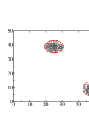
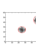
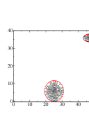
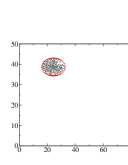
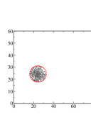
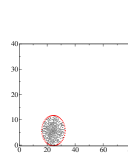
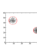
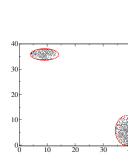
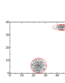
Figure 2: This plot shows all 10 2-dimensional sub-spaces of our 5-dimensional toy likelihood function with 2 minima in $\chi^{2}$. The black points are $\chi^{2}\leq\chi^{2}_{\text{lim}}$ found by APS after 10,000 samplings. The red contours are the known $\chi^{2}=\chi^{2}_{\text{lim}}$ contours of the function.

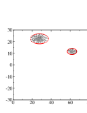
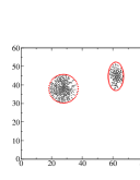
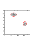
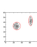
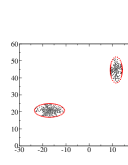
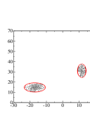
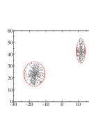
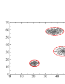
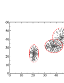
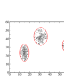
Figure 3: This plot shows all 10 2-dimensional sub-spaces of our 5-dimensional toy likelihood function with 3 minima in $\chi^{2}$. The black points are $\chi^{2}\leq\chi^{2}_{\text{lim}}$ found by APS after 10,000 samplings. The red contours are the known $\chi^{2}=\chi^{2}_{\text{lim}}$ contours of the function.

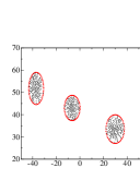
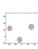
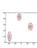
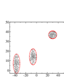
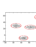
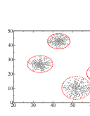
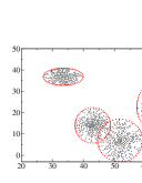
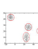
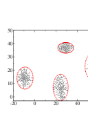
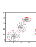
Figure 4: This plot shows all 10 2-dimensional sub-spaces of our 5-dimensional toy likelihood function with 4 minima in $\chi^{2}$. The black points are $\chi^{2}\leq\chi^{2}_{\text{lim}}$ found by APS after 10,000 samplings. The red contours are the known $\chi^{2}=\chi^{2}_{\text{lim}}$ contours of the function.

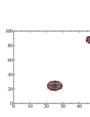
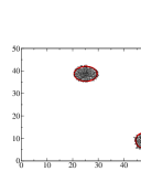
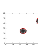
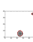
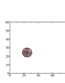
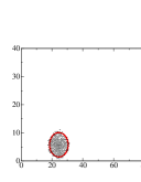
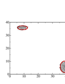
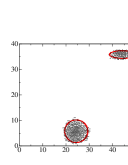
Figure 5: This plot shows all 10 2-dimensional sub-spaces of our 5-dimensional toy likelihood function with 2 minima in $\chi^{2}$. The black points represent the $95\%$ Bayesian credible limit found by APS (and determined as described in Section 2.4) after 10,000 samplings. The red contours represent the known $95\%$ Bayesian credible limit of the toy function.

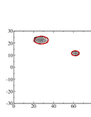
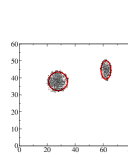
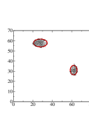
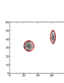
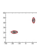
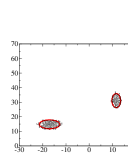
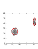
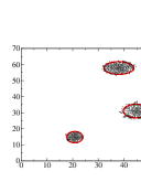
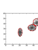
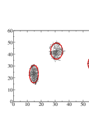
Figure 6: This plot shows all 10 2-dimensional sub-spaces of our 5-dimensional toy likelihood function with 3 minima in $\chi^{2}$. The black points represent the $95\%$ Bayesian credible limit found by APS (and determined as described in Section 2.4) after 10,000 samplings. The red contours represent the known $95\%$ Bayesian credible limit of the toy function.

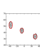
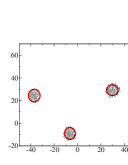
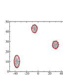
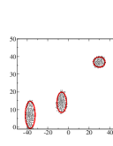
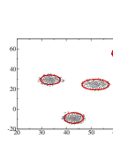
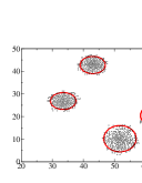
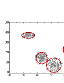
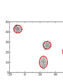
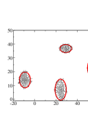
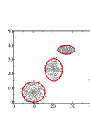
Figure 7: This plot shows all 10 2-dimensional sub-spaces of our 5-dimensional toy likelihood function with 4 minima in $\chi^{2}$. The black points represent the $95\%$ Bayesian credible limit found by APS (and determined as described in Section 2.4) after 10,000 samplings. The red contours represent the known $95\%$ Bayesian credible limit of the toy function.

5 A Real Example: WMAP

Section 4 demonstrates the robustness of APS against multi-modal $\chi^{2}$ functions. However, it does have some short-comings as a test of APS’s abilities. As was already noted, there are no interesting parameter degeneracies in equation (19). Furthermore, because this function was constructed artificially, there is no noise. At any point in parameter space, $\chi^{2}$ falls smoothly and monotonically towards the associated local minimum of $\chi^{2}$. To really have confidence in APS abilities, we must test it on actual physical data drawn from the universe, with all of the noisy and ill-behaved properties that entails. To that end, we will now consider for our $\vec{\theta}\rightarrow\chi^{2}$ function the likelihood function on the 7-year data release of the WMAP CMB satellite [Jarosik et al. 2011, WMAP 2010]. For simplicity, we consider only the anisotropy power spectrum of the temperature-temperature correlation function.

The parameter space we explore is the six-dimensional space of the spatially flat concordance $\Lambda$CDM cosmology:

• $\Omega_{b}h^{2}$ – the density of baryons in the Universe
  

• $\Omega_{\text{CDM}}h^{2}$ – the density of cold dark matter in the Universe
  

• $\tau$ – the optical depth to the surface of last scattering. $\tau$ cannot be constrained without polarization data, which we do not consider here. However, it functions as a nuisance parameter to be marginalized over. The fact that APS can handle it as well as MCMC is an important test of APS’s feasibility.
  

• $h$ – the Hubble parameter in units of $100~{}\text{km}~{}\text{s}^{-1}~{}\text{Mpc}^{-1}$
  

• $n_{s}$ – the spectral index controlling the distribution of scalar density perturbations in the Universe
  

• $\ln[10^{10}A_{s}]$ – the amplitude of the initial scalar density perturbations in the Universe

These are the parameters taken by the publicly available MCMC code CosmoMC, which we use to run our baseline MCMC chains [Lewis and Bridle 2002]. The $\vec{\theta}\rightarrow\chi^{2}$ function in this case involves converting these parameters into the power spectrum of anisotropy $C_{\ell}$s on the sky and comparing those $C_{\ell}$s to the actual measurements registered by the WMAP satellite. Using the (very fast) Boltzmann code CAMB to calculate the $C_{\ell}$s [Lewis et al. 2000] takes 1.3 seconds on a 2.5 GHz processor. Evaluating the $\chi^{2}$ using the likelihood code provided by the WMAP team [WMAP 2010] takes an additional 2 seconds (this can, of course, be sped up by using a faster machine and multiple cores). Hence the need for an algorithm like APS or MCMC to accelerate the search. We will consider both equations (14) and (16) as the covariogram for our Gaussian process, though we find that the choice has little effect on our results. We will also consider setting $\chi^{2}_{\text{lim}}=\chi^{2}+\Delta\chi^{2}$ as wel as setting $\chi^{2}_{\text{lim}}$ by hand.

To gauge the appropriateness of applying APS to this problem, we consider the two following tests. In Figure 8 we plot the minimum discovered value of $\chi^{2}$ yielded by APS and MCMC as a function of the number of samples drawn by each. If APS failed to find a suitable value of $\chi^{2}_{\text{min}}$, the use of $\Delta\chi^{2}$ to find $\chi^{2}_{\text{lim}}$ would be questionable. However, as we can see, the $\chi^{2}_{\text{min}}$ yielded by APS ($1273.3$) is within a few of the $\chi^{2}_{\text{min}}$ yielded by MCMC ($1270.7$).

The reader will note that MCMC discovers its $\chi^{2}_{\text{min}}$ much more rapidly than APS, however, we will see in Figures 10 through 12 that this rapid descent to $\chi^{2}_{\text{min}}$ does not translate into rapid convergence to the final credible limit. Because MCMC infers its limits based on the number of samples drawn from the Bayesian posterior probability, MCMC still requires many tens (or hundreds) of thousands of points to be sampled after $\chi^{2}_{\text{min}}$ has been discovered. Because it is learning the shape of the function directly, APS does not impose this requirement. The reader should also consider Figure 12, which shows the Frequentist confidence intervals discovered by APS when $\chi^{2}_{\text{lim}}$ is set by hand using prior knowledge of the size of the WMAP 7-year data set. In this case, APS does not need to learn $\chi^{2}_{\text{min}}$ in order to proceed. This is the original use case for which APS was designed. Here we see that the confidence intervals discovered agree very well with the Bayesian credible intervals discovered by MCMC.

The second question we consider is whether or not our assumption that $\vec{\theta}\rightarrow\chi^{2}$ can be modeled by a Gaussian process is valid. In Figure 9 we plot the average fractional error in $\mu$ as a proxy for $\chi^{2}$ as a function of the number of steps sampled (note: the vertical axis actually shows the average fractional error over the preceding 500 steps so that the early, imprecise models do not contaminate the later, precise models). As APS samples more points, its Gaussian process model becomes more accurate. This effect is more pronounced for covariogram (14) than for covariogram (16). However, we will see below that this difference does not affect the parameter constraints determined by APS.

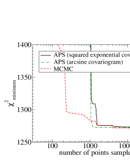
Figure 8: The minimum value of $\chi^{2}$ found by APS and MCMC on the WMAP 7 problem as a function of steps sampled by each.

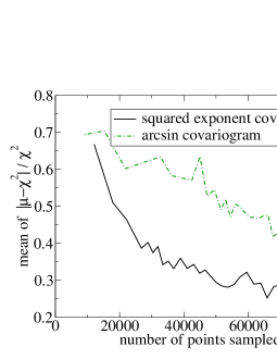
Figure 9: The average value of $|\mu-\chi^{2}|/\chi^{2}$ as a function of the number of points sampled by APS in the WMAP 7 problem. This is shown as a check on our assumption that $\vec{\theta}\rightarrow\chi^{2}$ can be approximated as a Gaussian process. Though the squared exponential covariogram (14) gives a better fit to the $\chi^{2}$ function than the arcsine covariogram (16), we see in Figures 10 and 11 that this has little effect on the parameter constraints derived by APS.

We now consider the ultimate results, namely the 95% confidence limits on our 6-dimensional cosmological parameter space yielded by APS. To provide a baseline against which to test APS, we run 4 independent MCMC chains using CosmoMC. Like the MCMC code used in Section 4, CosmoMC periodically adjusts its proposal density by learning the covariance matrix of the points it has already sampled. At each step, it proposes a new point in parameter space by randomly selecting an eigen vector of that learned covariance matrix and stepping along it. We integrate the posterior by taking the output chains, discarding the first 50% of steps as a burn-in period, and thinning the remaining steps so that we have a set of effectively independent samples drawn from the posterior. Quantitatively, this is determined by keeping only every $L$th sample after burn-in, where $L$ is set as the length such that the normalized correlation

$$\frac{\text{Cov}[\theta_{n}^{(i)},\theta_{n}^{(i+L)}]}{\text{Var}[\theta_{n}]}\leq 0.1$$ (20)

where $n$ is the index over the $N_{p}$ parameters and $(i)$ is the index over the samples drawn.

We find the 95% credible limits in two-dimensional slices of our parameter space using a total of 460,000 MCMC steps. These are assumed to be the true credible limits on the parameter space and are plotted as the thick red contours in Figures 10 through 12 below. Against these control contours, we plot the Frequentist confidence limits (all points with $\chi^{2}\leq\chi^{2}_{\text{lim}}$) discovered by APS after only 50,000 evaluations of $\chi^{2}$. We consider both an adaptive $\chi^{2}_{\text{lim}}=\chi^{2}_{\text{min}}+12.6$ (12.6 is the $\Delta\chi^{2}$ corresponding for 95% confidence limit in the case of 6 parameters) and an absoulte $\chi^{2}_{\text{lim}}=1280.7$ (this is the 95% confidence limit for a $\chi^{2}$ probability distribution with the 1199 degrees of freedom corresponding to the 1199 $C_{\ell}$s in the data set). These are the black points in Figures 10, 11, and 12 respectively. These confidence limits overlap very nicely with the true credible limits discovered by MCMC, comporting the the idea that, in the large data limit, Bayesian credible limits and Frequentist confidence limits ought to align.

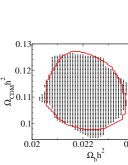
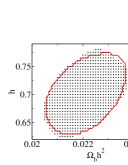
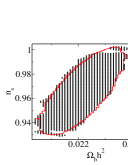
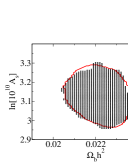
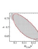
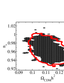
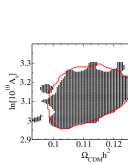
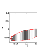
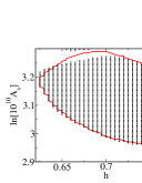
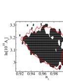
Figure 13: The 10 2-dimensional sub-spaces of our 6-dimensional parameter space ($\tau$ is ignored because no real constraint can be gleaned from this data). The thick red contours are the 95% Bayesian credible limits determined by MCMC after 460,000 calls to $\chi^{2}$. The black regions are the 95% Bayesian credible limits determined by MCMC after 50,000 calls to $\chi^{2}$.

For comparison of convergence properties, we plot the Bayesian credible limits discovered by MCMC after only 50,000 $\chi^{2}$ evaluations. These are the black regions in Figure 13. While MCMC has clearly converged to the final confidence limits in some of the 2-dimensional sub-spaces shown, others (Figures 13, 13, and 13) evince the presence of significant noise in the MCMC chains. Indeed, even the “final” credible limit contour (the red contour) in Figure 13 shows significantly more noise along the edges than, for instance, Figure 13. This is meant, not to disparage the convergence properties of MCMC, but to show that any convergence advantage MCMC may have over APS is not absolute. This should be compared with the clear advantage APS demonstrated over MCMC in identifying multi-modal likelihood functions in Section 4 above.

In Figure 14, we plot the 95% Bayesian credible limit discovered by APS after 50,000 evalutations of $\chi^{2}$ and determined by the method outlined in Section 2.4. Unfortunately, we do not see here the convergence to the true credible limits that we saw in Figures 5-7. While it does appear that APS has correctly identified the locations and general shapes of the true credible limits, it has, in most cases, drawn credible limits that are larger than those found by MCMC. This should not be surprising. APS was designed with Frequentist confidence limits in mind, and Figures 10-12 seem much better converged than Figure 14. However, it does seem that APS might be useful in cases where little prior knowledge is known about $\vec{\theta}\rightarrow\chi^{2}$ and users need to be confident that they have discovered all of the low-$\chi^{2}$ regions in a particular parameter space. Once APS has been used to identify rough Bayesian credible limits, more detailed algorithms (like MCMC) can be run using the prior knowledge gained by APS to refine the credible limits.

As a final note, we do not plot any confidence or credible limits for $\tau$. This is because $\tau$ needs CMB polarization data for meaningful constraints. For the sake of simplicity, we did not consider CMB polarization data here. Thus, $\tau$ has become a “nuisance parameter”: it affects the fit of our theoretical models, but cannot itself be meaningfully constrained. MCMC handles such parameters by effectively integrating over them when delivering the two-dimensional contours of Figures 10 through 12. APS handles such nuisance parameters by simply allowing them to vary and returning any combinations of useful-plus-nuisance parameters that satisfy the $\chi^{2}\leq\chi^{2}_{\text{lim}}$ criterion. The fact that this nuisance paramter did not significantly impede the convergence of APS relative to MCMC speaks well of APS’ ability to handle actual physical problems which often include parameters that have little physical interest but are required to, e.g., calibrate noise distributions or systematics.

We reiterate that the purpose of this section was to demonstrate that the presence of real-world noise in the data and likelihood function do not significantly impede APS’s ability to determine confidence and credible limits. The problem of drawing parameter constraints from the WMAP likelihood function is, by now, well-understood, and shrewdly drawn priors and proposal densities are readily available. Indeed, prior knowledge of early WMAP results allowed us to use the following initial proposal densities for the MCMC runs displayed in this section:

$$\Omega_{\text{b}}h^{2} = 0.03\pm 0.005$$ (21)

$$\Omega_{\text{CDM}}h^{2} = 0.1\pm 0.05$$

$$\theta = 1.0\pm 0.01$$

$$\tau = 0.07\pm 0.03$$

$$n_{s} = 0.95\pm 0.05$$

$$\ln\left[10^{10}A_{s}\right] = 3.0\pm 0.2$$

where $\theta$ is 100 times the ratio of the sound horizon to the angular diameter distance and recombination (this is the input parameter CosmoMC uses in place of $h$). These distributions are fairly similar to the final, marginalized, one-dimensional distributions of those same parameters

$$\Omega_{\text{b}}h^{2} = 0.0221\pm 0.0006$$

$$\Omega_{\text{CDM}}h^{2} = 0.112\pm 0.006$$

$$\theta = 1.039\pm 0.003$$

$$\tau = 0.05\pm 0.03$$

$$n_{s} = 0.96\pm 0.02$$

$$\ln\left[10^{10}A_{s}\right] = 3.12\pm 0.07$$

$$h = 0.7\pm 0.03$$

Conversely, for the purposes of our APS runs, we initialize the algorithm only with the gross assumptions that

$$0.01\leq \Omega_{\text{b}}h^{2} \leq 0.04$$ (22)

$$0.01\leq \Omega_{\text{CDM}}h^{2} \leq 0.3$$

$$0.4\leq h \leq 1.0$$

$$0.005\leq \tau \leq 0.15$$

$$0.7\leq n_{s} \leq 1.3$$

$$2.0\leq \ln\left[10^{10}A_{s}\right] \leq 4.0$$

In less well-studied problems, users may not understand their parameter spaces well enough to be able to supply shrewd proposal densities in the vein of equations (21). In such a situation, the exploratory behavior of APS demonstrated in Section 4 may prove more important than the theoretical rigor offered by MCMC’s sampling algorithm.

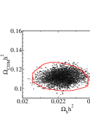
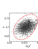
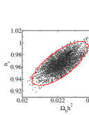
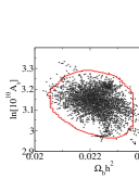
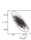
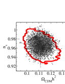
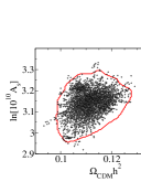
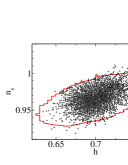
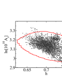
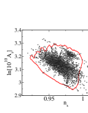
Figure 10: The 10 2-dimensional sub-spaces of our 6-dimensional parameter space ($\tau$ is ignored because no real constraint can be gleaned from this data). The thick red contours are the 95% Bayesian credible limits determined by MCMC after 460,000 calls to $\chi^{2}$. The black points are the 95% Frequentist confidence limits determined by APS after 50,000 calls to $\chi^{2}$. $\chi^{2}_{\text{lim}}=\chi^{2}_{\text{min}}+12.6$. Equation (14) is used for the Gaussian process covariogram.

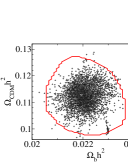
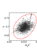
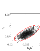
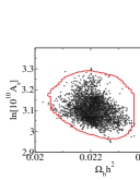
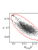
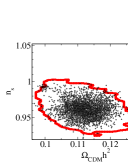
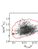
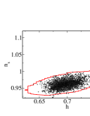
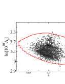
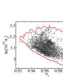
Figure 11: The 10 2-dimensional sub-spaces of our 6-dimensional parameter space ($\tau$ is ignored because no real constraint can be gleaned from this data). The thick red contours are the 95% Bayesian credible limits determined by MCMC after 460,000 calls to $\chi^{2}$. The black points are the 95% Frequentist confidence limits determined by APS after 50,000 calls to $\chi^{2}$. $\chi^{2}_{\text{lim}}=\chi^{2}_{\text{min}}+12.6$. Equation (16) is used for the Gaussian process covariogram.

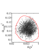
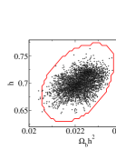
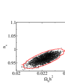
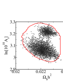
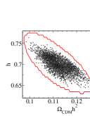
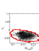
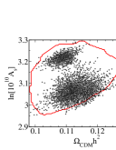
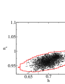
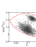
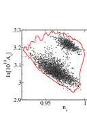
Figure 12: The 10 2-dimensional sub-spaces of our 6-dimensional parameter space ($\tau$ is ignored because no real constraint can be gleaned from this data). The thick red contours are the 95% Bayesian credible limits determined by MCMC after 460,000 calls to $\chi^{2}$. The black points are the 95% Frequentist confidence limits determined by APS after 50,000 calls to $\chi^{2}$. $\chi^{2}_{\text{lim}}=1280.7$. Equation (14) is used for the Gaussian process covariogram.

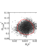
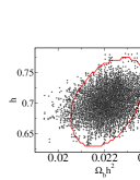
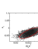
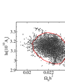
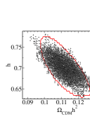
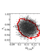
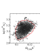
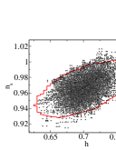
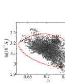
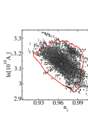
Figure 14: The 10 2-dimensional sub-spaces of our 6-dimensional parameter space ($\tau$ is ignored because no real constraint can be gleaned from this data). The thick red contours are the 95% Bayesian credible limits determined by MCMC after 460,000 calls to $\chi^{2}$. The black points are the 95% Bayesian credible limits determined by APS according to the method outlined in Section 2.4. While the APS credible limit covers the entire MCMC limit, it also covers regions of parameter space excluded by MCMC.

6 Conclusions

In Section 4 we indicated that, consistent with the findings of Bryan et al. (2007), APS is more robust than MCMC against multi-modal likelihood functions (at least on the idealized cartoon $\vec{\theta}\rightarrow\chi^{2}$ functions considered). In Section 5, we showed that the presence of realistic noise does not interfere with APS’s ability to derive Frequentist confidence limits. However, the Bayesian credible limits yielded by APS remain noisy and imprecise. We believe that this performance can still be of use to the community, especially when trying to evaluate proof-of-concept parameter constraints (perhaps for forecasting parameter constraints from future experiments) with very expensive $\vec{\theta}\rightarrow\chi^{2}$ functions on poorly-understood parameter spaces. Certainly, for users interested in plotting Frequentist confidence limits, APS is a viable option.

There remain, however, several concerns to be addressed in the use of APS. Unlike MCMC, there is no obvious criterion for convergence of the APS algorithm. One possibility is to interpret the Frequentist confidence limit as a hyperbox (i.e. keep track of the allowable maximum and minimum values of each parameter as $\chi^{2}=\chi^{2}_{\text{lim}}$ is explored) and watch the growth of the volume of that hyperbox as a function of the number of $\vec{\theta}\rightarrow\chi^{2}$ evaluations. Figure 15 plots this convergence metric for the APS run in Figure 10. While it appears that APS may have converged after $\sim$50,000 evaluations, the volume of the Frequentist confidence limit continues to grow, though Figure 10 already shows good coverage of the control Bayesian credible limit. It is, of course, possible that we are seeing the effect of the slight difference between the Bayesian credible limit and the Frequentist confidence limt, even in the large-data case.

Figure 15: The parameter space volume of the Frequentist confidence limit in figure 10 as a function of the number of $\vec{\theta}\rightarrow\chi^{2}$ evaluations.

Another concern is that, while APS was explicitly designed to rapidly converge to the Frequentist confidence limit (where rapidity is measured in the number of $\vec{\theta}\rightarrow\chi^{2}$ evaluations made), the searches in Section 2 are complicated enough that they will add extra clock time to each $\vec{\theta}\rightarrow\chi^{2}$ evaluation. We have attempted to balance APS so that it does not rely too heavily on expensive calculations. However, some overhead is inevitably required. Figure 16 shows the average overhead time in seconds added by APS to each $\vec{\theta}\rightarrow\chi^{2}$ evaluation as a function of the number of evaluations. As the number of evaluations grow and the number of points APS must search when constructing its Gaussian processes also grows, so does this extra time (the initial spike is due to the first expensive call to the hyper-parameter optimization in Section 3.2). Though the extra time stays within the bounds of a few 0.1 seconds per $\vec{\theta}\rightarrow\chi^{2}$ evaluation, this may still be too expensive in the case of functions for whom a direct $\vec{\theta}\rightarrow\chi^{2}$ takes a vanishingly small amount of time.

Figure 16: The extra time added by APS to a $\vec{\theta}\rightarrow\chi^{2}$ as a function of the number of $\vec{\theta}\rightarrow\chi^{2}$ evaluations.

Finally, one advantage of MCMC that APS cannot overcome is its comparative ease to implement. To this end, we make our code available at https://github.com/uwssg/APS/. The code is presented as a series of C++ classes with directions indicating where the user can interface with the desired $\vec{\theta}\rightarrow\chi^{2}$ function. Those with questions about the code or the algorithm should not hesitate to contact the authors.

Appendix A Frequentist Confidence Intervals

Frequentist confidence limits are not nearly as common in the astrophysical literature as their Bayesian counterparts. For this reason, we define them below.

Suppose we are going to conduct some experiment resulting in a random data set $\vec{d}$. Suppose also that we have some theory by which the distribution of $\vec{d}$ is controlled by a set of parameters $\vec{\theta}$. We would like to use $\vec{d}$ to make some statement about the true values of $\vec{\theta}^{(0)}$ i.e., the values of $\vec{\theta}$ actually realized by the universe. Rather than adopt the Bayesian perspective and talk about the peak and width of the the posterior “probability of $\vec{\theta}$ given $\vec{d}$,” Frequentists attempt to construct sets of estimators $\vec{\theta}^{(\text{CL})}(\vec{d})$ such that the probability that $\vec{\theta}^{(0)}\in\vec{\theta}^{(\text{CL})}(\vec{d})$ is $(1-\alpha)\%$, i.e. if the experiment were repeated many times, yielding many different sets $\vec{d}$, and the confidence limit set $\vec{\theta}^{(\text{CL})}$ was calculated for each of those data sets, the true value of $\vec{\theta}^{(0)}$ would fall within $\vec{\theta}^{(\text{CL})}$ $(1-\alpha)\%$ of the time. This is the original definition of confidence intervals posited by Neyman (1937; see his equation 20 and the attendant discussion). It also underlies the confidence belt construction discussed in Chapter 9 of Eadie et al. (1971), Chapter 20 of Stuart and Ord (1991) and section II B of Feldman and Cousins (1998).

The specific example we consider in Section 5 of this paper is the WMAP 7 year data release measuring the anisotropy in the Cosmic Microwave Background. This data set takes the form of a power spectrum composed of 1199 $C_{\ell}$s ($2\leq\ell\leq 1200$) characterizing the anisotropy power on different angular scales. These 1199 measurements represent independent Gaussian random variables. The probability density on $C_{\ell}$ space associated with measuring a particular set of $C_{\ell}$s given a particular candidate set of $\vec{\theta}^{(c)}$ is

$$P\propto\exp\big{[}-\frac{1}{2}\sum_{\ell,\ell^{\prime}}(C_{\ell}(\vec{d})-C_{\ell}(\vec{\theta}^{(c)}))\text{Cov}^{-1}_{\ell\ell^{\prime}}(C_{\ell^{\prime}}(\vec{d})-C_{\ell^{\prime}}(\vec{\theta}^{(c)}))\big{]}$$

where $C_{\ell}(\vec{d})$ are the 1199 measured values of $C_{\ell}$, $C_{\ell}(\vec{\theta}^{(c)})$ are the 1199 values of $C_{\ell}$ predicted by the candidate theory, and $\text{Cov}^{-1}_{\ell\ell^{\prime}}$ is the inverse of the covariance matrix relating the measured $C_{\ell}$s. A change of variables to

$$\chi^{2}\equiv\sum_{\ell\ell^{\prime}}(C_{\ell}(\vec{d})-\vec{C}_{\ell}(\vec{\theta}^{(c)}))\text{Cov}^{-1}_{\ell\ell^{\prime}}(C_{\ell^{\prime}}(\vec{d})-C_{\ell^{\prime}}(\vec{\theta}^{(c)}))$$

gives the well-known result that the 1199 independent, Gaussian-distributed $C_{\ell}$s give a $\chi^{2}$ statistic distributed according to the eponymous $\chi^{2}$ distribution with 1199 degrees of freedom. The $\chi^{2}$ distribution is well-understood. In the case of 1199 degrees of freedom, 95% of the probability is enclosed by $\chi^{2}\leq 1280.7$. We may use this fact to construct a 95% confidence limit.

Recall the definition of Frequentist confidence limits. The true value of the parameters $\vec{\theta}^{(0)}$ is fixed, but $\vec{d}$ (in the specific example above, the set of 1199 $C_{\ell}$s) is random and will change each time we conduct the experiment. In this case, “conducting the experiment” means creating a new Universe with a new Cosmic Microwave Background, randomly generated from the same $\vec{\theta}^{(0)}$, and measuring it with WMAP; while this is impossible, we ask the readers to suspend their disbelief for the sake of this illustration. Because of what we have just noted about $\chi^{2}$, in 95% of our repeated WMAP experiments $\chi^{2}$ calculated relative to the true parameter set $\vec{\theta}^{(0)}$ will be less than or equal to 1280.7. If, for each set of $C_{\ell}$s we find all of the combinations of $\vec{\theta}$ that yield $\chi^{2}\leq 1280.7$, that set of $\vec{\theta}$ will contain $\vec{\theta}^{(0)}$ 95% of the time. Taking our one realization of $C_{\ell}$ and finding all of the values of $\vec{\theta}^{(\text{CL})}$ which give $\chi^{2}\leq 1280.7$, we can be confident that we have contained $\vec{\theta}^{(0)}$ with 95% probability. This is what is meant by a 95% Frequentist confidence limit.

In the large data limit, Frequentist confidence limits are expected to give comparable results to Bayesian inference (as we see in Figure 10). In the limit of small data, Frequentist confidence limits may differ from Bayesian limits. If statistical fluctuations dominate the signal, it is possible for Frequentist methods to return an empty confidence limit (no points in parameter space fit the data). While this may seem an unpalatable outcome, it is useful to know that one’s data set is noisy so that one can interpret the explored likelihood surface with all due caution. Lyons (2002 and 2008) discusses this distinction, as well as the comparative strengths and weaknesses of other statistical perspectives, at greater length than this work.

The Frequentist approach to confidence limits described herein is actually a conservative version of the non-parametric confidence ball approach popular among academic statisticians (see the introduction to Baraud 2004). Statisticians typically are concerned with using data to constrain the form of a function in arbitrary function space. They use the data to derive an estimator of the function from which it was drawn (in our example, the smooth theoretical $C_{\ell}$ function) and then use theoretical considerations to draw a hypersphere in function space about that fit constituting the $(1-\alpha)\%$ confidence limit [Beran and Dümbgen 1998, Li 1989, Baraud 2004, Cai and Low 2006, Davies et al. 2009]. Note that these hyperspheres (referred to in the literature as “confidence balls”) are calculated from the data alone without reference to any underlying physical model or set of (in Wilks’ 1938 words) “admissible hypotheses.” In this way, they function identically to the $\chi^{2}$ test adopted in the present work.

Astrophysicists can utilize the “confidence ball” formalism by demanding that their theoretical models give predicted functions that fall within the hypersphere drawn in function space. This is how Bryan et al. (2007) originally drew their constraints on the CMB. It is also how Genovese et al. (2004) confirmed the statistical significance of the harmonic peaks in the WMAP 1-year CMB data. Because the confidence hypersphere is drawn a-priori, without any consideration for the admissible hypotheses within the space of physical parameters, this method would be straightforward to interface with APS (indeed, it was included in the Bryan et al. draft of the code). We leave such an implementation to future work.

The more familiar Likelihood Ratio Test detailed by Wilks (1938) and Neyman and Pearson (1933) is an asymptotic simplification of Frequentist confidence limits for cases in which we know that the true model must exist within some limited set of hypotheses. In this case, one assumes that the adopted $\vec{\theta}$ parametrization is the only possible way of explaining that data. In that case, the $\chi^{2}_{\text{min}}$ on parameter space must, by definition, be the smallest achievable $\chi^{2}$. $\Delta\chi^{2}\equiv\chi^{2}-\chi^{2}_{\text{min}}$ is then distributed according to the $\chi^{2}$ distribution with $N_{p}$ degrees of freedom. This is the assumption underlying our use of $\Delta\chi^{2}$ in the test of Section 4 and 5 above.

References

- [Baraud 2004] Baraud, Y. 2004, Annals of Statistics 32 528
- [Bentley 1975] Bentley, J. L. 1975, Communications of the Associaton for Computing Machinery 18, 509
- [Beran and Dümbgen 1998] Beran, R. and Dümbgen, L. 1998, Annals of Statistics 26 1826
- [Bergé et al. 2012] Bergé, J., Price, S., Amara, A., and Rhodes, J. 2012, Monthly Notices of the Royal Astronomical Societ 419, 2356
-
[Bryan 2007]
Bryan, B., 2007, Ph.D. thesis, Carnegie Mellon University,
http://reports-archive.adm.cs.cmu.edu/anon/ml2007/abstracts/07-122.html - [Bryan et al. 2007] Bryan, B., Schneider, J., Miller, C. J., Nichol, R. C., Genovese, C., and Wasserman, L., 2007, Astrophys. J. 665, 25
- [Cai and Low 2006] Cai, T. T. and Low, M. G. 2006, Annals of Statistics 34 202
- [Davies et al. 2009] Davies, P. L., Kovac, A., and Meise, M. 2009, Annals of Statistics, 37 2597
- [Eadie et al. 1971] Eadie, W. T., Drijard, D., James, F. E., Roos, M., and Sadoulet, B., 1971, “Statistical Methods in Experimental Physics” (North-Holland, Amsterdam).
- [Feldman and Cousins 1998] Feldman, G. J. and Cousins, R. D. 1998, Phys. Rev. D. 57 3873
- [Feroz and Hobson 2008] Feroz, F. and Hobson, M. P., Monthly Notices of the Royal Astronomical Society, 384, 449
- [Feroz et al. 2009] Feroz, F., Hobson, M. P., and Bridges, M. 2009, Monthly Notices of the Royal Astronomical Society, 398, 1601
- [Genovese et al. 2004] Genovese, C. R., Miller, C. J., Nichol, R. C., Arjunwadkar, M., and Wasserman, L. 2004, Statistical Science 19 308
- [Gilks et al. 1996] Gilks, W. R., Richardson, S., and Spiegelhalter, D. J. ed., “Markov Chain Monte Carlo in Practice,” (Chapman & Hall, 1996), Boca Raton, F.L.
- [Habib et al. 2007] Habib, S., Heitmann, K., Higdon, D., Nakhleh, C., and Williams, B. 2007, Physical Review D 76 083503
-
[James 1972]
James, F. 1972, Proceedings of the CERN Computing and Data Processing School,
http://seal.web.cern.ch/seal/documents/minuit.mntutorial.pdf - [Jarosik et al. 2011] N. Jarosik et al., 2011, Astrophys. J. Suppl. Ser. 192 14
- [Li 1989] Li, K.-C. 1989, Annals of Statistics 17 1001
-
[Lewis and Bridle 2002]
Lewis, A. and Bridle, S., 2002, Phys. Rev. D 66, 103511;
http://cosmologist.info/cosmomc/readme.html - [Lewis et al. 2000] Lewis, A., Challinor, A., and Lasenby, A., 2000, Astrophys. J. 538, 473
-
[Lyons 2002]
Lyons, L. 2002, “Bayes or Frequentism?”
http://www-cdf.fnal.gov/physics/statistics/statistics_recommendations.html - [Lyons 2008] Lyons, L. 2008, Annals of Applied Statistics, 2 887 [arXiv:0811.1663]
- [Marsaglia 2003] Marsaglia, G. 2003, Journal of Statistical Software, 8 14
- [Nelder and Mead 1965] Nelder, J. A. and Mead, R. 1965, The Computer Journal, 7 308
- [Neyman and Pearson 1933] Neyman, J. and Pearson, E. S. 1933, Philosophical Transactions of the Royal Society of London, Series A, 231 289
- [Neyman 1937] Neyman, J. 1937, Philos. Trans. R. Soc. London A236 333. Reprinted in “A Selection of Early Statistical Papers of J. Neyman” (University of California Press, Berkeley, 1967)
- [Press et al. 2007] Press, W. H., Teukolsky, S. A., Vetterling, W. T. and Flannery, B. P. 2007, “Numerical Recipes” (3d edition), Cambridge University Press, 2007
-
[Rasmussen and Williams 2006]
Rasmussen, C. E. and Williams, C. K. I., 2006, “Processes for Machine Learning”
http://www.GaussianProcess.org/gpml - [Shafieloo et al. 2012] Shafieloo, A., Kim, A. G., and Linger, E. V. 2012, Physical Review D 85, 123530 [arXiv:1204.2272]
- [Stuart and Ord 1991] Stuart, A. and Ord, J. K., 1991, “Classical Inference and Relationship,” 5th ed., Kendall’s Advanced Theory of Statistics, Vol. 2 (Oxford University Press, New York).
-
[WMAP 2010]
WMAP, 2010
http://lambda.gsfc.nasa.gov/product/map/dr4/m_products.cfm - [Wilks 1938] Wilks, S. S. 1938, Annals of Mathematical Statistics, 9 60