Macroscopic Coherent Rectification in Andreev Interferometers
Abstract
We investigate nonlinear transport through quantum coherent metallic conductors contacted to superconducting components. We find that in certain geometries, the presence of superconductivity generates a large, finite-average rectification effect. Specializing to Andreev interferometers, we show that the direction and magnitude of rectification can be controlled by a magnetic flux tuning the superconducting phase difference at two contacts. In particular, this results in the breakdown of an Onsager reciprocity relation at finite bias. The rectification current is macroscopic in that it scales with the linear conductance, and we find that it exceeds 5% of the linear current at sub-gap biases of few tens of ’s.
pacs:
74.45.+c, 74.78.Na, 73.23.-bThe presence of superconductivity often magnifies quantum coherent effects in transport. Examples include Aharonov-Bohm oscillations in the conductance Pet93 ; Har96a ; Naz96 and in the thermopower Eom98 ; Par03 ; Sev00 ; Vir04 ; Tit08 ; Jac10 , coherent backscattering Bee95 ; Har98 and resonant tunneling Goo08 . The mechanism behind this enhancement can be traced back to Andreev reflection And64 which generates new (diffuson-like) contributions to the transmission, that are sensitive to different phases in the superconducting order parameter or to external magnetic fluxes Naz96 ; Sev00 ; Vir04 ; Tit08 ; Jac10 ; Eng11 . These contributions are proportional to the number of transmission channels. In purely metallic systems, quantum coherent effects are of order one or smaller, they are therefore negligible in the limit of large linear conductances Imry .
Novel quantum coherent effects in transport have recently been uncovered in the form of nonlinear contributions to the current-voltage characteristic. Of particular interest are contributions that are odd in a magnetic field , with San04 ; Spi04 ; And06 ; Zum06 ; Let06 ; Ang07 . They originate from electronic interactions which, under finite applied biases, modify the local potential landscape inside the conductor. The associated rectification coefficient has been found to be proportional to the energy derivative of a transmission coefficient , and in metallic quantum dots, it is accordingly sample-dependent, with a vanishing average and fluctuations decreasing with , San04 ; Spi04 . Because is odd in , its presence results in the breakdown of an Onsager reciprocity relation Ons31 at finite bias, . According to Mott’s law, at low temperature the thermopower is also proportional to the energy derivative of the transmission Ash67 . Therefore, the question that naturally arises is whether the enhancement of the thermopower observed in mesoscopic systems contacted to superconducting islands Eom98 ; Par03 ; Sev00 ; Vir04 ; Tit08 ; Jac10 , translates into a similar magnification of nonlinear rectifying contributions to the conductance. This is the problem we focus on in this manuscript.
We investigate weakly nonlinear transport in coherent metals connected to superconducting contacts. We find that the presence of superconductivity renders the rectification current finite on average and macroscopically large – in the sense that it scales with the linear conductance . The emergence of a finite does not require to break time-reversal symmetry in the metallic part of the system. It takes place, for instance, for two superconducting contacts with phase difference , . The physics behind this effect is that, in Andreev systems, finite biases not only modify the local potential landscape in the metal Chri96 ; Pil02 , they also affect the electrochemical potential of the superconductor. In the case of a superconducting island, adjusts itself to ensure current conservation, and therefore transmission coefficients now depend on the absolute energy of the charge carriers, the local potential landscape in the metal and additionally on . Our key observation is that rather generic hybrid systems can be devised where Andreev reflection results in a large, finite-average derivative of with respect to the quasiparticle excitation energy , . These contributions are similar to those giving a finite-average thermopower in Andreev interferometers Jac10 ; Eng11 . The theory we are about to present predicts maximal average rectification currents amounting to 5–10% of the linear current at still moderate, sub-gap biases of 10–30 V, and for which superconducting correlations persist over distances of several microns. In purely metallic systems, fluctuating rectification effects on the order of 2% typically occur for biases in the range 0.1–1 mV Zum06 ; Let06 ; Ang07 .
We consider two models of Andreev interferometers, where two metallic terminals indexed are connected to mesoscopic (either chaotic ballistic or disordered diffusive) quantum dots via leads carrying transmission channels. The dots have no particular spatial symmetry and are ideally connected to two -wave superconducting contacts with pair potentials , each carrying channels. Physical properties depending only on phase differences, we set and with . We consider a single superconducting island with two contacts into which no current flows on time average in steady-state. The models are sketched in Fig. 1. We consider the regime where the temperature is much smaller than the pair potential, the latter being in its turn much smaller than the Fermi energy, . At low bias, , the quasiparticle excitation energy is then always much smaller than . Accordingly, we assume perfect Andreev reflection at the superconducting contacts.
Both our models are specifically devised to correlate the average time an electron takes on its way from one lead to a superconducting contact, with the phase at that contact. This is achieved by the introduction of ballistic necks, which quasiparticles at the Fermi level cross in a time . These necks are indicated by dashed lines in Fig. 1. The way action and Andreev reflection phases are correlated is easy to see by considering electrons at an excitation energy , injected from the left terminal and Andreev reflected back to it. From Fig. 1 we see that, if Andreev reflection occurs at the right superconducting contact, these electrons acquire a total phase that is larger by an amount than if they hit the left superconducting contact. Such correlations were shown in Ref. Jac10 to generate large, finite-average contribution to the thermopower for finite . We show below that they also result in a finite-average rectification.
The starting point of our analysis is the scattering theory formula for the electric current in terminal Cla96 (we set and express electric currents in units of )
| (1) |
with quasiparticle indices for electrons and for holes, the Fermi function for a -quasiparticle and the positive-defined quasiparticle excitation energy, . We introduced transmission coefficients for a -quasiparticle injected from lead to an -quasiparticle exiting in lead . In the presence of superconductivity, transmissions will depend on (i) the energy of the injected quasiparticle, (ii) the local potential landscape on the quantum dot, and (iii) the electrochemical potential on the superconductor. We take as our reference energy and express the transmission probabilities in terms of two energy differences, , which describes how transmission is affected by the local potential landscape and the quasiparticle’s excitation energy.
At low but finite bias we expand Eq. (1) to quadratic order in and write the current as
| (2) |
The linear, , and quadratic, conductances are given by
| (3a) | |||||
| (3b) | |||||
with
| (4a) | |||||
| (4b) | |||||
The linear conductance has been calculated earlier (see e.g. Refs. Jac10 ; Eng11 ), and we focus our attention on the nonlinear term. The second term in the parenthesis in Eq. (3b) gives the screening contribution to the nonlinear conductance, self-consistently generated by the voltage biases and the Coulomb interaction Chri96 . It can be rewritten as Chri96 ; San04
| (5) |
For metallic mesoscopic cavities the derivative of the transmission with respect to the local potential is random from one ensemble member to another, furthermore, for large , it is not correlated to the local potential fluctuations San04 . This is not modified by the presence of superconductivity, therefore, . The screening term has no average effect on the current, and we neglect it from now on. The first term in Eq. (3b) is the bare contribution to the nonlinear conductance Chri96 . In contrast to the purely metallic case, it depends on the derivative of the transmission with respect to the quasiparticle excitation energy counted from the chemical potential of the superconductor. Below we find that the bare term gives a dominant, finite-average contribution to the nonlinear conductance. We thus rewrite Eq. (2) as
| (6) |
with
| (7) |
Eq. (6) expresses electric currents through the normal leads as a function of the superconducting chemical potential . In steady-state, the latter is self-consistently determined by current conservation at the normal leads. The next step is thus to determine and insert its value into Eq. (6). One gets an explicitly gauge invariant expression
| (8) |
with the bias voltage and
| (9a) | |||||
| (9b) | |||||
It is easily checked that the expression for reproduces the result of Ref. Cla96 . To calculate the rectification coefficient we follow the trajectory-based semiclassical approach of Refs. Jac10 ; Whi09 and compute the dominant contributions to leading order in the ratio of the total number of transport channels in the left and right superconducting contacts ( and ) and in the normal contacts ( and ). The corresponding diagrams are shown in Fig. 2.
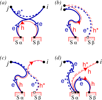
Eqs. (8–9) apply to both interferometers shown in Fig. 1, however, the coefficients are geometry-dependent and we now calculate them in both cases, starting with the asymmetric single-cavity interferometer. For the interferometer of Fig. 1a, we find, to leading order in , and ,
| (10a) | |||||
| (10b) | |||||
with a thermal damping integral
| (11) |
The value of the integral decreases with the temperature, , and the dwell time, , through the cavity. When one has . For a given temperature, it is largest when [when coth]. We see from Eq. (10b) that, when is nonzero, a finite average rectification current flows. This current is odd in . Both finite and are required for this current to occur, because they both are necessary to correlate action and Andreev phases. This correlation is key to obtaining a finite-average in Eq. (7). Eq. (10b) further shows that when , =L, R, SL, SR, and for sufficiently asymmetric normal terminals, , the rectification current is macroscopically large, .
We next present our results for the double-cavity interferometer. We find, again to leading order,
| (12a) | |||||
| (12b) | |||||
where is the number of channels in the neck connecting the two cavities and the thermal damping integral is given this time by
| (13) |
Here, for simplicity, we took the same dwell time, , for both cavities. ¿From Eq.(12b), we see that a macroscopic rectification effect also occurs in this geometry – under similar conditions as above, i.e. that for =L, R, C, SL and SR, and sufficiently asymmetric superconducting contacts, – and that when , rectification effects in the two geometries of Fig. 1 have the same thermal damping, .
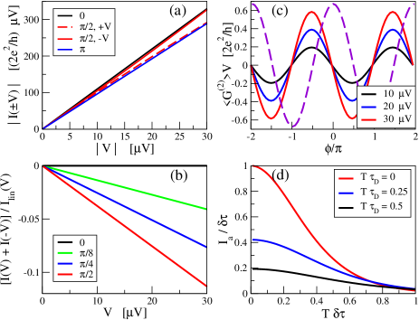
We illustrate our results in Fig. 3 for the asymmetric
single-cavity model. We first show
the current as a function of applied bias in Fig. 3a, for and .
We see that a rectification effect of more than 5% occurs at and bias voltage of
30 V. This is rendered more evident in Fig. 3b, which
shows the relative current asymmetry , normalized by the
linear current as a function of bias voltage. We see that
at still moderate biases (well below the superconducting gap of Al, and corresponding to a
coherence length ranging from tens to hundreds of m for GaAs 2DEG to 3D metals),
the rectification effect
exceeds 5%.
We next show in Fig. 3c the rectification current as a function of
for three different voltages , 20, and 30V. In contrast to
the mesoscopic rectification effects in metallic quantum dots which are random
in an applied magnetic field San04 ; Spi04 ; Zum06 ,
we see that the presence of superconductivity induces a regular behavior of
as a function of , with the magnitude of the effect increasing with bias. Finally, the damping of the rectification with temperature is
illustrated in Fig. 3d.
Our approach to weakly nonlinear transport is closely related to the one pioneered by Büttiker and Christen Chri96 . One important difference is that we here took advantage of the presence of superconductivity to Taylor-expand the currents in voltages measured from the superconducting potential . This directly enforces gauge invariance at our level of approximation, where the screening term in Eq. (3b) is neglected. Current conservation is furthermore satisfied in our treatment by unitarity of the scattering matrix, , and by the condition (self-consistently determining ) that no current enters the superconducting island on time average in steady state. In Ref. Chri96 , voltages are taken from an arbitrary potential as there is no superconductor. In that case gauge invariance is only satisfied after a self-consistent determination of the local potential landscape and of the dependence of transmission coefficients on external voltage biases via the latter.
We have presented a theory for weakly nonlinear transport in hybrid metallic/superconducting systems and shown that there can be a finite average rectification for such systems. We found that, in contrast to purely metallic mesoscopic systems, the presence of superconductivity generates potentially large, , finite-average rectification effects. The latter can furthermore be tuned in magnitude and direction by an external magnetic flux. Alternatively, we note that this effect leads to the breakdown of an Onsager relation, with (still in units of ) for the asymmetric single-cavity model and for the double-cavity model. We expect the rectification effect we predict to be experimentally testable in Andreev interferometers such as those of Refs. Har96a ; Eom98 ; Par03 .
This work was supported by the NSF under grants DMR-0706319 and PHY-1001017 and by the Swiss Center of Excellence MANEP. It is our pleasure to thank M. Büttiker and P. Stano for discussions.
References
- (1)
- (2) V.T. Petrashov, V.N. Antonov, P. Delsing, and T. Claeson, Phys. Rev. Lett. 70, 347 (1993).
- (3) S.G. den Hartog, C.M.A. Kapteyn, B.J. van Wees, T.M. Klapwijk, and G. Borghs, Phys. Rev. Lett. 77, 4954 (1996).
- (4) Y.V. Nazarov and T.H. Stoof, Phys. Rev. Lett. 76, 823 (1996).
- (5) J. Eom, C.-J. Chien, and V. Chandrasekhar, Phys. Rev. Lett. 81, 437 (1998).
- (6) A. Parsons, I.A. Sosnin, and V.T. Petrashov, Phys. Rev. B 67, 140502(R) (2003).
- (7) R. Seviour and A. F. Volkov, Phys. Rev. B 62, R6116 (2000).
- (8) P. Virtanen and T. Heikkilä, Appl. Phys. A 89, 625 (2007).
- (9) M. Titov, Phys. Rev. B 78, 224521 (2008).
- (10) Ph. Jacquod, R. S. Whitney, Europhys. Lett. 91 67009 (2010).
- (11) C.W.J. Beenakker, J.A. Melsen, and P.W. Brouwer, Phys. Rev. B 51, 13883 (1995).
- (12) S.G. den Hartog, B.J. van Wees, Yu.V. Nazarov, T.M. Klapwijk, and G. Borghs, Physica B 249, 467 (1998).
- (13) M.C. Goorden, Ph. Jacquod, and J. Weiss, Phys. Rev. Lett. 100, 067001 (2008); Nanotechnology 19, 135401 (2008).
- (14) A.F. Andreev, Sov. Phys. JETP 19, 1228 (1964).
- (15) T. Engl, J. Kuipers, and K. Richter, Phys. Rev. B 83, 205414 (2011).
- (16) Y. Imry, Introduction to Mesoscopic Physics, 3rd Ed. (Oxford University, Oxford, 2008).
- (17) D. Sanchez and M. Büttiker, Phys. Rev. Lett. 93, 106802 (2004).
- (18) B. Spivak and A. Zyuzin, Phys. Rev. Lett. 93, 226801 (2004).
- (19) A.V. Andreev and l.I. Glazman, Phys. Rev. Lett. 97, 266806 (2006).
- (20) D. Zumbühl, C.M. Marcus, M.P. Hanson, A.C. Gossard, Phys. Rev. Lett. 96, 206802 (2006).
- (21) R. Leturcq, D. Sanchez, G. Götz, T. Ihn, K. Ensslin, D.C. Driscoll, and A. C. Gossard, Phys. Rev. Lett. 96, 126801 (2006).
- (22) L. Angers, E. Zakka-Bajjani, R. Deblock, S. Guéron, H. Bouchiat, A. Cavanna, U. Gennser, and M. Polianski, Phys. Rev. B 75, 115309 (2007).
- (23) L. Onsager, Phys. Rev. 38, 2265 (1931).
- (24) N.W. Ashcroft and N.D. Mermin, Solid-State Physics (Saunders College Publishing, Philadelphia, 1967).
- (25) T. Christen and M. Büttiker, Europhys. Lett. 35, 523 (1996).
- (26) S. Pilgram, H. Schomerus, A.M. Martin, and M. Büttiker, Phys. Rev B 65, 045321 (2002).
- (27) N. R. Claughton and C. J. Lambert, Phys. Rev. B 53, 6605 (1996).
- (28) R. S. Whitney, P. Jacquod, Phys. Rev. Lett. 103, 247002 (2009).