Improved numerical methods for infinite spin chains with long-range interactions
Abstract
We present several improvements of the infinite matrix product state (iMPS) algorithm for finding ground states of one-dimensional quantum systems with long-range interactions. As a main new ingredient we introduce the superposed multi-optimization (SMO) method, which allows an efficient optimization of exponentially many MPS of different length at different sites all in one step. Hereby the algorithm becomes protected against position dependent effects as caused by spontaneously broken translational invariance. So far, these have been a major obstacle to convergence for the iMPS algorithm if no prior knowledge of the systems translational symmetry was accessible. Further, we investigate some more general methods to speed up calculations and improve convergence, which might be partially interesting in a much broader context, too. As a more special problem, we also look into translational invariant states close to an invariance braking phase transition and show how to avoid convergence into wrong local minima for such systems. Finally, we apply the new methods to polar bosons with long-range interactions. We calculate several detailed Devil’s Staircases with the corresponding phase diagrams and investigate some supersolid properties.
pacs:
02.70.-c, 03.67.-a, 67.85.-dI Introduction
A numerical method for the simulation of large quantum systems needs to meet two requirements: i) an ansatz suitable for the problem in question, and ii) efficient algorithms to find the (at least nearly) optimal solution within the chosen ansatz. For one-dimensional quantum systems on lattices, the currently most powerful numerical tools are matrix product states (MPS) based algorithms including the density matrix renormalization group (DMRG) Schollwoeck (2011); White (1992); Fannes et al. (1992); Affleck et al. (1987); Dukelsky et al. (1998). Their primary limitation is given by the amount of entanglement they can handle. Several extensions of MPS have been conceived to overcome this restriction as, (e.g. Vidal (2007a); Hübener et al. (2009, 2010)), but for most practical applications MPS are still the first choice. This is mainly due to the performance of the underlying optimization routines. Although the general task to find ground states is known to be NP hard Eisert (2006); Schuch et al. (2008), commonly used algorithms seem to have no problem to attain optimal MPS solutions within computer precision for a plenitude of physical relevant systems. Nevertheless, for some physical systems of interest these algorithms still face severe difficulties.
In this paper, we treat such problematic cases given by ground states of infinite spin chains with long-range interactions. An increasing interest in reliable numerical methods for these states is, e.g., triggered by the excellent experimental control of ultracold gases and the possibility to realize systems with long-range dipole-dipole interactions such as Rydberg atoms or polar molecules Burnell et al. (2009); Schachenmayer et al. (2010); Trefzger et al. (2011). Although these systems are of finite size, one is often interested in the thermodynamical limit (i.e., infinite systems) for a better insight.
Different strategies are known for the numerical study of ground states in the thermodynamic limit. One might try to extrapolate results from a series of increasingly large finite systems Cardy (1996); Pirvu et al. (2012); Gendiar et al. (2011) or directly construct the infinite state itself. The latter is, e.g., done by the infinite time-evolving block decimation (iTEBD) algorithm Vidal (2007b), which is based on an explicit translational invariant ansatz. This ansatz is quite elegant for interactions which are restricted to nearest neighbors, while it gets impractical for long-range interactions.
A comfortable way to incorporate long-range interactions is to encode them into a matrix product operator (MPO) McCulloch (2007); Murg et al. (2010); Crosswhite and Bacon (2008); Fröwis et al. (2010). This concept can be integrated in an infinite matrix product state (iMPS) algorithm Crosswhite et al. (2008); McCulloch .
The basic idea of this iMPS algorithm is to obtain the ground state of an infinite system as the fixed point of a constantly growing finite state by inserting iteratively new sites into its middle until convergence is reached. A major disadvantage of this approach is that the algorithm generally fails to converge if the ground state has a non-trivial translational symmetry.
In this paper, various extensions to the basic iMPS algorithm are presented. As a central element, the superposed multi-optimization (SMO) is introduced (section III.2), which provides a remedy for the just mentioned convergence problem. Here, the key idea is to join the optimization of exponentially many MPS in a superposition and solve it efficiently. Due to this superposed optimization, the effective overall problem becomes translational invariant again and poses no longer a hindrance for convergence.
We also introduce several improvements which work independently of the SMO method. As such, we present two different modifications of the MPS optimization routine: On the one hand, we use physical insight for systems close to translational invariance breaking phase transition to suggest a method to reduce the danger of being trapped into a local minimum of the energy (section III.4). On the other hand, we provide a more technical discussion how to recycle information from previous optimizations to speed up calculations (section IV.3). As a part of these considerations we provide a simple implementation of a Davidson like algorithm Sleijpen and Van der Vorst (2000) based on information from previous optimizations (appendix D). This implementation is not bonded to the MPS framework and hence might be used in much broader context.
All algorithms are described in depth, such that readers who are willing to reproduce our results should find all the information needed for successful programming. As a consequence, readers who just like to understand the crucial ideas might find the amount of algorithmic details far beyond their interest. Having these two types of readers in mind, we partitioned the material according to its level of detail into different chapters, such that entire passages can be omitted.
In section II, we review the basic concepts and the iMPS algorithm as presented in Crosswhite et al. (2008). Readers who feel save to skip this part find in Fig. 1 and Fig. 2 a pictorial description of all symbols used in this section. In Section III, the main new concepts of this paper are presented, above all the SMO method. Changes of the algorithm are kept to a minimum in here in contrary to section IV where several algorithmic improvements and their numerical realization are presented in detail. Each subsections of section IV contains an individual topic, which is presented in the first lines. These subsections can be skipped without danger of losing the ability to understand the rest of the paper. A slight exception might be section IV.3, in which the concept of iterative eigenvector solver based on subspace projections is reviewed. Familiarity with this concept is assumed in section IV.4, IV.5 and appendix B.1. In section V, we apply our new algorithm to a system of polar bosons with long-range interactions. Detailed calculations of Devil’s Staircases and phase diagrams are shown and a supersolid like phase is investigated. Finally, the paper is complemented by an appendix, into which several details have been outsourced.
II Basic algorithm
In this section we review fundamental concepts Schollwoeck (2011) and the iMPS algorithm as presented in reference Crosswhite et al. (2008). For this algorithm to work not only the Hamiltonian but also the ground state have to be translational invariant. The extension to ground states with broken translational symmetry will be introduced in section III.
II.1 MPS and MPO
In this paper we deal with spin chains. The quantum state of a spin chain is determined by the inner degrees of freedom of its components
| (1) |
Since the size of the tensor grows exponentially with the number of sites, a more economical representation is needed. A matrix product state (MPS) Schollwoeck (2011); Fannes et al. (1992); Affleck et al. (1987) consists in the ansatz
| (2) | |||||
where we used the Einstein summation convention. For a general exact quantum state exponentially growing bond dimensions are needed, but even for infinite systems excellent approximations are possible with moderate bond dimensions if the ground state fulfills an area law for the entanglement entropy Hastings (2007).
For Hamiltonians
| (3) |
a similar ansatz as for the quantum state (2) leads to the concept of matrix product operators (MPO) McCulloch (2007); Murg et al. (2010); Crosswhite and Bacon (2008); Fröwis et al. (2010)
| (4) | |||||
Many relevant Hamiltonians are represented by MPO with relative small bond dimensions. For our purposes, it is important to mention that this is often also true for Hamiltonians with long-range interaction terms (see, e.g., Fröwis et al. (2010)). A recipe for the explicit construction is explained in Appendix A. In the case of a translational invariant Hamiltonians (see remark below), the MPO can be built in such a fashion that all tensors are identical for . This allows us to drop the index in the square brackets except for the leftmost and rightmost tensors.
| (5) | |||||
Further more, all tensors are independent of the total number of sites. As a consequence, the MPO of a translational invariant Hamiltonian for sites can easily be augmented to sites by just inserting another tensor .
Apart from an efficient representation of quantum states and operators, MPS and MPO also provide an efficient way to calculate expectation values. For details, we refer to the literature (as, e.g., Schollwoeck (2011)).
Remark: In this paper we apply the term translational invariant also to finite systems (with open boundary conditions) and their Hamiltonians which are used in the iMPS algorithm to approach the infinite case.
II.2 Overview of the iMPS algorithm
Any algorithm which deals with infinite MPS could be addressed as iMPS algorithm. In this paper we use this term exclusively for algorithms of the type as presented in reference Crosswhite et al. (2008). This algorithm aims at finding an MPS representation for the ground state of an infinite one-dimensional quantum system. In its plain version the iMPS algorithm takes translational invariance for granted such that all sites behave equally. Thus all we need to construct the entire state is a perfect description of one site and its entanglement features with its environment given by the rest of the system. This environment is dominated by nearby neighbor sites while the influence of sites far away can be neglected in any one-dimensional system with an asymptotic decay of correlations faster than . Therefore the environment built up by an infinite system can be simulated with a finite system. Correspondingly the center site of a sufficiently large but finite system provides a good approximation for its counterpart in the infinite case.
The iMPS algorithm is built upon a finite system, which is iteratively enlarged by inserting new sites into its middle. Since we express quantum states by MPS each of these new sites is represented by an individual tensor (2). Before a new tensor is inserted it is optimized such that the resulting energy
| (6) |
is minimized. Hereby all previously inserted tensors are left unchanged. Of course, these local optimizations of the new tensors are generally not sufficient to find the lowest energy state of the entire system. What we are supposed to get is a ground state approximation which might be bad at the outer edges but close to the center, it should become better with each new tensor inserted. This is all we need to obtain an adequate description of the center site’s environment, since the influence of the outer sites fades away with distance, anyway. Therefore, we expect the environment of the center site to converge towards its infinite counterpart, and with that the new tensors inserted into each round should converge, too
| (7) |
For ground states which violate translational invariance, it is no longer given that all sites behave equally. At this point, our intuitive argumentation breaks down and the algorithm generally fails to converge. We will study this case in section III. For the time being, we assume that the algorithm ends up with a converged tensor . With the help of this one tensor, the entire iMPS can be constructed using the rules we will encounter in II.3.
II.2.1 Long-range interactions
An important ingredient for a fast computer code is a clever book-keeping of the interaction terms, which allows us to save many calculations due to recycling. In the case of long-range interactions, this task becomes tricky, since the iMPS algorithm permanently splits the MPS and adds new sites. By this means, the distances between sites on the left and right halves change each time and with them all distance-dependent interaction terms. Nonetheless, for translational invariant Hamiltonians recycling can still be done in a well-arranged fashion by encoding the Hamiltonian into an MPO as in equation (5). Every time the MPS is enlarged by a new tensor, the MPO is enlarged by the standard tensor , too. This simple procedure automatically corrects all distance-dependent interaction terms.
II.3 Constructing the MPS
So far, we just mentioned that the iMPS algorithm constructs the MPS by constantly inserting new tensors in its middle. We will now specify on that. First, it is convenient to treat the MPS as divided into two halfs, left and right from the center. Each time the optimization procedure described in II.4 provides a new tensor , we have to decide into which half is to be absorbed. This is done under the following rules:
- 1.
-
2.
With each new tensor overwrite the of the tensor before.
Each is optimized in such a fashion that it compensates for the overwritten .
For the orthogonalization (9) we proceed as follows: In a first step, we write the tensor as matrix where is a multi-index. If the tensor is to be absorbed into the left MPS half elsewise . For the leftmost and rightmost tensors of the MPS, which have only two indices, . The index corresponds to the leftover index of , which is not in . Next, the matrix is decomposed into an orthogonal part and a “rest” part . Different decompositions would fulfill this task, but for the working of the algorithm it is best to resort to a singular value decomposition
| (10) | |||||
Rewritten as tensors we end up with equation (8).
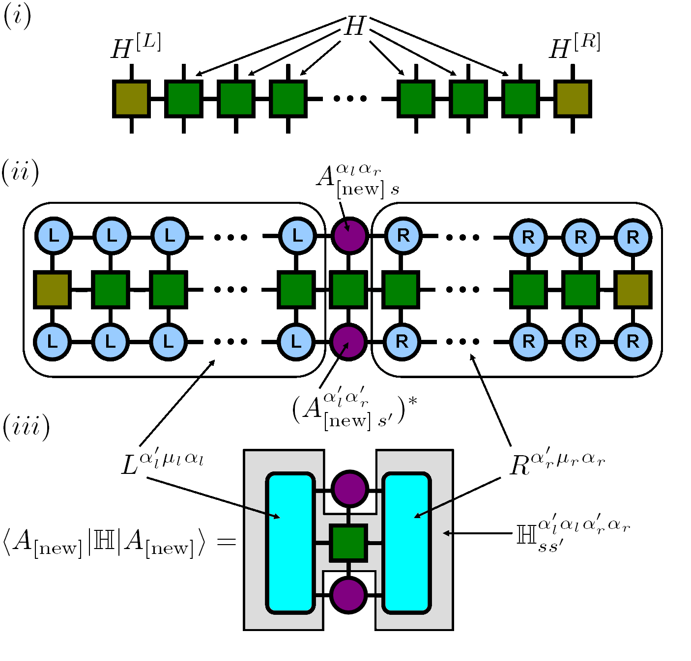
A consequent application of these rules yields an MPS built of orthogonalized tensors and one single matrix from the very last in the center (Fig. 1 ).
| (11) |
This MPS standard form is numerical robust and has an easily calculated norm . To see this let us multiply (the left half of equation (11)) with its complex conjugated
| (12) | ||||
and analog for the right half. Thanks to equation (9) all -pairs turn into -functions and the norm of the MPS (11) equals the remaining (see Fig. 1 ) which also equals the norm of the last inserted tensor . Thus
| (13) |

II.4 Tensor optimization
The iMPS algorithm is an iterative procedure. As described in section II.2 new tensors are constantly inserted into the MPS, which represents the finite state . Each of these new tensors is optimized such that the energy is minimized. As we will discuss in more detail below, this can be written as
| (14) |
-
•
is the vectorized form of the tensor , that is with the multi-index
-
•
is an effective operator built of the MPO representation of the Hamiltonian (5) and all MPS tensors of and except for the two new .
-
•
is the identity operation thanks to the orthogonalized standard form of the MPS, see (12).
Equation (14) is solved by setting equal to the lowest eigenvector of .
Remark: We will repeatedly use the notation or for a vectorized tensor .
II.4.1 Effective operator
In II.3 we mentioned that it is convenient to treat the MPS as divided into two halves: left and right from the newest tensor . For the same reason we decompose into a left half and a right half , which are connected by a single MPO tensor (5) corresponding to the new site (see Fig. 2 ).
| (15) |
with .
Since the iMPS algorithm is an iterative procedure, and are built up iteratively, as well. Suppose we intend to absorb the of the previous optimization step into the left half. First, we use equation (8) to gain the orthogonal tensor . With that
| (16) |
where the asterisk denotes complex conjugation. In this case, where the tensor is absorbed into the left half, the right half stays unchanged . Obverse, if we decide to absorb into the right half, the left half stays unchanged and becomes
| (17) |
II.5 Algorithm
After having presented the decisive ingredients of the iMPS algorithm, we like to emphasize the steps one actually has to perform on the computer. The algorithm consists of an initializing procedure (see II.5.2) and an iteration loop, which is repeated until convergence is reached (7). The tensor is all we need to calculate expectation values. We do not hold any copy of the MPS we are calculating. The only objects stored (in the purest version of the algorithm) are the actual versions of (16), (17) and .
II.5.1 Loop
-
1.
Calculate the new with . Therefor
-
(a)
Use (15) to calculate .
-
(b)
Set equal to the lowest eigenvector of
-
(a)
-
2.
Decide, whether to absorb into the left or right half (e.g. even steps left, odd steps right) and act accordingly in the following two steps.
- 3.
- 4.
II.5.2 Initialization
At the beginning we have to initialize the values of and . This can be done with the help of an exact solution for a small system best with an even number of sites (we mostly used for two-level sites). The state is split into a left and right part, which allows to calculate and . In more details, note the following:
-
1.
Write the Hamiltonian of the small system as matrix with multi-indices and solve for .
-
2.
Split the multi-index in two multi-indices, giving , which can be interpreted as a matrix.
-
3.
Use a singular value decomposition (or Takagi’s factorization if ).
-
4.
Interpret the index structure of as .
-
5.
, (5).
-
6.
Use analog to to calculate .
Comparing with (11) we find that
III Broken translational invariance
In this section, we present some new concepts for the iMPS algorithm which arise from the need to deal with spontaneously broken translational invariance. A principal shortcoming of the basic iMPS algorithm is its failure to converge in such cases. To overcome this deficiency, we introduce the superposed multi-optimization (SMO) method in section III.2. Once convergence is restored, we turn our attention in section III.3 to the question of how to obtain a specific solution out of the ground state manifold degenerate due to broken translational invariance. In addition, in section III.4, we treat the special case of a non-degenerate ground state which is separated by a very small energy gap from a state that breaks translational invariance.
III.1 Preliminary considerations
Just one tensor suffices to construct an entire iMPS. At first sight, one might therefore think that such an iMPS is only capable of describing states where all sites behave equally, which is no longer true for states which break translational invariance. But still, also these states can be handled. This is due to the construction rules presented in section II.3. These result in an iMPS structure given by equation (11), where the matrix marks a special position (and with that breaks translational invariance) if it can not be commuted to its neighbor sites.
The real problem is to find . In II.2, we already mentioned that our argumentation in favor of the convergence is no longer valid in the case of broken translational invariance. The iMPS algorithm is grounded on local optimization and therefore it is vulnerable to locally altering states, as they appear on a physical level for states with broken translational invariance. In this case, simple local optimization will not result in a global optimal fixed point .
III.1.1 Known solutions
When we write about the breakdown of translational invariance, we mean that the state is no longer invariant under the shift of one site. Still, the state can maintain invariance under the shift of sites. If is known, one can introduce new super sites where one super site encompasses of the old sites. Now, the system is translational invariant with respect to the shift of one super site. This involves that we have to optimize tensors which represent the super sites. Due to the exponential increase of the physical dimension, this method is practical for very small only. To avoid the scaling problem, Crosswhite Crosswhite et al. (2008) suggested to use an MPS ansatz for the super sites. In practice this means, we insert old sites at once and optimize the corresponding tensors. We are not aware if this was ever tested successfully. Aside from that, one still needs a prior knowledge of the value .
Alternatively, one can extend the standard MPS structure with auxiliary tensors Ueda et al. (2011); Ueda and Maruyama (2012), which allow us to introduce a symmetry breaking element for the price of a non-linear optimization. To our knowledge, this has not been tested for long-range interactions, so far.
III.2 Superposed multi-optimization (SMO)
Our solution of the convergence problem induced by locally altering states does not depend on any prior knowledge and stays within the standard MPS framework. The key idea is to wash out local dependency of the optimization by choosing each new tensor such that it minimizes the sum of the energy of exponentially many different MPS instead of just one. These MPS are different ground state approximations to the qualitatively same Hamiltonian applied to systems of different sizes. All necessary minimizations can be joined in a superposition and solved by one optimization. The time relevant steps stay the same as in the single MPS optimizing algorithm presented so far, so there is no noticeable loss in speed.
As explained in the following, after each optimization round, the number of MPS joined in the superposition increases by a factor of 4. Thus, in the th round, the optimization (14) gets formally extended to
| (18) |
The MPS representing the are of different length and the position of the tensor is no longer in the center but varies from MPS to MPS. In the basic algorithm, the tensors experience quite individualized environments and the optimization adapts to these local circumstances. In the modified algorithm, faces exponentially many different environments averaging out local effects and emphasizing common global features. This enforces heavily the desired convergence .
III.2.1 Modification of the algorithm
Formally, the superposition in equation (18) is based on different MPS. These MPS are not hand picked, but indirectly generated by the algorithm. The only modification needed to create such a superposition concerns the left and right halves and . We still use equation (16) and (17) to perform the iteration steps and but afterwards we add the new and the old results to achieve superpositions
| (19) |
Since this is a simple addition of two tensors, the structure and size of and stay the same and do not entail any computational complications.
In the basic algorithm we have to decide at each iteration step whether to absorb the tensor into the left half (16) or into the right half (17). Only the half of choice is modified. Now, we symmetrize the algorithm and modify both halves in each step. With this modification, the operator sum is calculated with one single use of equation (15). As a further advantage of the symmetrization the modified iMPS algorithm can now take advantage of mirror symmetric Hamiltonians. As this subject is a bit off-topic, we refer the interested reader to Appendix F.
Since each of the tensors is absorbed into the left half and the right half the longest MPS encoded in the operator superposition of contains tensors (where we neglect the contribution from the initialization routine explained in section II.5.2 and the hole for the new tensor ). But in the general MPS each of the tensors only appears with a probability of due to the addition of the new and old and in equation (19). The possible tensor combinations give rise to the heralded different MPS from which are of length . More precisely of these MPS contain tensors left and tensors right from the hole for the new tensor .
III.2.2 Comments
The crucial observation is that the iteration steps to perform are always the same independent of the tensor position and the size of the MPS. Therefore all the different MPS can be optimized together combined in a superposition. The reader who is more familiar with finite MPS calculations might wonder about the complete loss of information concerning the single MPS in the superposition, which comes along with equation (19). We have to remind ourselves that the main objective of the iMPS algorithm is to get the tensor , which suffices to construct the infinite MPS. The finite MPS are just tools to obtain this tensor. Once we have it the finite MPS are no longer needed.
Another interesting question is whether the operator sum in equation (18) constructed via equation (19) is really suitable for a variational ansatz. This question has two aspects.
-
1.
Is every optimal iMPS solution of equation (18) also a minimum of the Hamiltionian?
-
2.
Does the algorithm always converge to this optimal solution?
The intuitive argumentation given in section II.2 also suggests that the answer to the second question should be yes, but actually even for the well-established DMRG algorithm the answer has to be no, since otherwise NP hard problems could be solved. Nonetheless, it is a matter of fact that DMRG converges extremely well for most practical purposes. The same "practical proof" can be given for equation (18) as demonstrated by our applications (section V).
The first question can be answered more formally. Equation (18) represents the sum of exponentially many energy terms. The lowest conceivable value of this sum is reached, if each energy term takes its individual minimal value. If all individual energies are minimized, the obvious answer to the first question is yes. Hence, we have to ask, whether it is possible to minimize all individual energies at once, having in mind that all MPS involved are created indirectly via equation (19). With finite MPS this might only be possible up to a certain relative error. But for the limit of infinite MPS this relative error shrinks to zero and the problem is trivially solved by uniform iMPS, i.e., in the case where all tensors stem from the same . Then, all iMPS appearing in equation (18) look alike and either none or all of them minimize their Hamiltonians. Even in the case of broken translational invariance, one can always find at least one translational invariant ground state, which can be written as uniform iMPS and hence optimizes all terms in the sum at once.
Next, we like to further inspect the numerical consequences of equation (19) for the different MPS which are part of the operator sum . The tensor was absorbed into exactly half of the superpositions encoded in and in . Since and are the building blocks of (15), four subsets of can be distinguished:
-
1.
was neither absorbed into nor into
-
2.
was only absorbed into
-
3.
was only absorbed into
-
4.
was absorbed into both halves and .
Although we never experienced any practical problems, the cases 1 and 4 are, at least from the theoretical point of view, a bit troublesome. In case 4 the tensor is inserted twice. But was never optimized for double insertion. Close to the end, when is almost achieved, this should pose no problem. Meanwhile, at an early stage the effect should be more severe. On the other hand, even in the basic algorithm, the MPS description is not perfect – especially not at the beginning.
Case 1 might seem trivial, since everything stays the same. Potential difficulties arise in the superposition with the other cases. According to equation (8) the tensors are decomposed into and and only is absorbed. The matrix is overwritten with the next (respectively ). In the basic algorithm, this is easy to justify: The next can compensate for . But, a perfect compensation can only be achieved for one , not for many of them. Here is the problem: In case 1, old of the previous steps are conserved, while in 2., 3. and 4. a new comes into play. All have to be compensated for. The stronger the alter, the less adequate is their compensation. The variation of the can be reduced by enforcing to be small. Towards the end of the optimization is small anyway. At an early stage one might have to resort more strongly to the convergence enforcing method we will discuss in section IV.1.2.
III.3 Selecting a specific ground state
We have seen how to ensure convergence in the case of broken translational symmetry. But so far, we have no control to which of the degenerate ground states the algorithm converges. Some of these ground states might be more favorable for our purposes than others, and we now answer the question as to how to obtain them. Any further degeneration aside from broken translational invariance is excluded from this consideration.
Let us look at two fully converged MPS and where be a representation of the wished-for ground state which fits our purposes best, while stands for any ground state to which the algorithm actually has converged. According to equation (11), both MPS have the following structure
| (20) |
In Appendix C, we show that it suffices to replace the matrix in by the new matrix to obtain an MPS which represents exactly the same physical state as
| (21) |
In other words, we do not need to take care to which ground state the algorithm converges, since after it has converged, we are able to transform the obtained solution easily into any other. We do not even have to know , as long as we have a description such as, e.g., “the ground state with the highest expectation value for the operator ”. All we have to do is a one-time optimization of the new matrix under the desired side condition.
III.3.1 One tensor update versus multi tensor update
So far, we focused on uniform MPS which result from an algorithm that inserts one new tensor each round. Crosswhite Crosswhite et al. (2008) suggested that one might also insert a certain number of tensors per round in the form of a small MPS. Although we are so far not aware of any successful practical applications of this ansatz, it is worth having a closer look. For the single-site algorithm to work in the presence of broken translational, invariance we introduced the SMO method, which washes out local variations and thereby fortifies convergence. Still, the SMO is a general method and could also be implemented in an -site algorithm.
As we have seen in the section above, the single-site iMPS algorithm will come up with a solution that encodes all possible ground states. This abundance has its price. Given the situation that we know the periodicity of the ground state of interest, we could use an iMPS algorithm which inserts sites at once. This would enable us to find some specific lowly entangled ground states which could be expressed by a non-uniform MPS with a far smaller bond dimension. Since translationally shifted copies of such a non-uniform MPS always allow us to construct a uniform MPS, the maximal gain in bond dimension is given by a factor and the maximal difference in the entanglement entropy of the half chain is . We could confirm this difference for the model studied in the applications (section V) varying the matrix (20) over the set of ground states, as described in the section above.
From the perspective of the needed bond dimension, the multi-tensor update is clearly superior to the-single tensor update for systems with a periodicity . Sill, in this paper we favor the single-tensor update, which needs no prior knowledge of the periodicity and results in a well-converging algorithm, which has proofed its reliability in practical tests.
III.3.2 Degenerate tensor
In the case of broken translational, invariance one can jump from one ground state solution to another just by changing the matrix , which is part of the bigger tensor (8). Hence, different minimize , i.e., is degenerate. The iMPS algorithm aims for the convergence . Without precautions, this convergence might be undermined towards the very end by an which jumps from one solution to another. At a first glance, this does not seem troublesome, because all solutions could jump to are good solutions. Nonetheless, due to imperfect numerics this jumping might also occur into of minor quality. This effect is not fatal, but it still might turn an otherwise perfect result into a less accurate one.
III.4 Translational invariant ground states and local minima
In this section, we consider possible convergence problems due to translational invariance breaking states which lie closely above the non-degenerate ground state level. In such cases, the infinite system still provides a translational invariant ground state, while for finite systems even small alterations of the energy spectrum due to boundary effects suffice to favor a ground state with broken translational invariance. Since the iMPS algorithm is based on growing finite systems, it might start out converging into a false minimum and get trapped there. Even if the algorithm escapes out of this trap later, it supposably costs many optimization rounds and significantly slows down convergence.
To avoid these problems we suggest to modify the algorithm such that it only converges to translational invariant states. This is no limitation: In the case of an unique ground state, the sole solution has to be translational invariant, anyway. If the ground state level is degenerate, one of the solutions is translational invariant and according to equation (21) we can still transform it into another type of solution after the algorithm has converged.
Whether the fully converged MPS ,
| (22) |
is translational invariant or not depends on its matrix . At this point we should be more precise and write or , depending on whether stems from a left or a right decomposition (8). Actually, as a consequence of decomposition (8) the MPS is translational invariant if the left and right version of are identical
| (23) |
In this case can be commuted to any position and hence does no longer mark any specific site of the MPS. This is what we are aiming for.
In order to end up with an where we alter the minimization routine which computes the tensors such that solutions with small differences i.e. big overlap are preferred. In the long run this should accumulate to .
As a first straight forward way we tried to extend the minimization (18) of to
| (24) |
with a suitable coupling parameter . This is no longer a simple to solve bilinear problem since one needs to perform the decomposition (10) to get and . To avoid this complication and restore bilinearity we tried to resort to the easily calculated approximations and (127) derived in the appendix E, but the results we obtained in this way were not very convincing.
In section IV.4 we introduce a less conventional approach which turned out to work far more satisfyingly for us. Instead of extending the minimization of by a new term as suggested in equation (24), we alter the routines of the iterative eigenvector solver we use to solve it. The modus operandi of these solvers is reviewed in section IV.3. Until after then, we suspend further explanations.
IV Enhanced algorithm
The considerations of the last section were mainly conceptual. The only actual change of the algorithm we performed is given by equation (19), which incorporates the SMO method. In this section, we delve far more into numerical details and extend the algorithm by further routines to make it more efficient. A reader not interested in technical details of the algorithm might proceed directly to section V
IV.1 Enforcing convergence
The goal of the iMPS algorithm is the global convergence . This property has to emerge over the long term, while it is not part of the evaluation system of the local minimization from which each is drawn. As a consequence, small local improvements might be purchased with strong fluctuating counteracting global convergence. In an unstable scenario of overcompensation, these fluctuations might even inflate in a fatal manner. To prevent this from happening we extend the algorithm by two methods. The first method (superposition method) aims at attenuating the influence of problematic on the ongoing calculations, while the second method (gain function method) directly modifies the optimization routine such that excessive variation of the are suppressed. Both methods are complementary and worked well together in our calculations.
IV.1.1 Superposition method
The first method takes advantage of the fact that the (18) of the modified algorithm represent superpositions of operators. By decreasing the weight of those contributions to the superpositions which contain problematic , one can ensure that excessive fluctuation of the do not spread to the level of the and with that inhibit a chain of overcompensation. We remind the reader that is absorbed into (16) and (17) before equation (19) is used to build up superpositions. This latter equation is now replaced by
| (25) |
The only new ingredient compared to equation (19) is the adjustable weight calculated as
| (26) |
where measures the deviation of and is a weighted average of the previous deviations. Each time the deviation exceeds the average value , gets smaller than 1 and with that the weight of all contributions of which contain is reduced accordingly.
To measure the deviation we need to define a reference tensor such that . In order to avoid unnecessary fluctuation of this reference tensor we use the same trick as above and define iteratively as a weighted average of the previous
For equation (26) to work we still have to define the weighted average . Various definitions are possible. As a heuristic choice, we picked the following one:
| (28) |
with . Obviously the term prevents a too sudden increase of by limiting it to per round. Without this term we get the clearer expression , i.e. older lose each round of their influence in the weighted average.
Finally, we remark that we end up in a deadlock if . To prevent this from happening we will introduce the parameter in equation (30) of the upcoming subsection.
IV.1.2 Gain function method
The idea of the gain function method is to manipulate the minimization procedure of by adding a gain function i.e. replacing by
| (29) |
where is the vectorized version of the reference tensor defined in equation (27). Let be the result of the above optimization. Obviously, bigger values for favor smaller deviations .
In the appendix B we show how to approximate efficiently such that
| (30) |
where and are parameters of our choice. Limiting by assigning e.g. (28) ensures that (26) is lower bounded around .
Assigning the parameter (30) allows us to shorten to a chosen fraction of the maximal value . The price to pay for a is a lesser energy improvement which is calculated as the difference between the energy one gets due to choosing instead of just taking
| (31) | |||||
Choosing e.g. a which corresponds to reduces by while the energy improvement is still at of the maximal value .
The parameter (30) and the entire superposition method are designed to intervene only in case that suddenly increases with ongoing – otherwise they have no effect. The parameter on the other hand always effects the calculation if chosen to be smaller than 1. Generally the should be chosen in dependence of (the bigger , the smaller and vice versa). Just for orientation (not as exclusive choice) we give the value we chose for most of our calculations
| (32) |
With that since . This formula was found heuristically and worked fine for us, although more adequate choices might exist.
When the iMPS algorithm finally approaches its end becomes very small and its effect might be overruled by numerical imprecision. To prevent this, we recommend defining a lower limit for above the limit of the numerical precision.
IV.2 Energy overgrow
If the average energy per site of an infinite state does not equal zero, the total energy of the entire state is . Of course, we never have to deal with an infinite value since our numeric is restricted to finite systems. Nonetheless, a problem remains. In the long run, the numeric value of all the information encoded in the tensor stays more or less the same except for the energy, which grows with each new site. The tensor gets more and more ill conditioned since the numeric value of the energy overgrows other information and thereby reduces the achievable precision. To avoid this problem, we advise to subtract each iteration step the energy from the system. Simply speaking, we recommend to assign
| (33) |
But to be of any use, this simple assignment has to be encoded into and the building blocks of (15). This can be done by modifying the MPO tensor used in equations (16) and (17). As shown in Appendix A, the MPO tensor has a slot which represents a local interaction term. To this local interaction we add .
IV.3 Minimization routine and information recycling
With an increasing number of rounds the successive minimizations of the different become more and more similar, which opens the opportunity to speed up the minimization recycling information from preceding turns. In order to understand these ideas (and also those of section IV.4, section IV.5, and Appendix B.1), we have to review the principles of the iterative eigenvector solvers we use Saad (2003). In the MPS context, these solvers come with the major advantage that never has to be constructed explicitly; it suffices to be able to assemble for any given . Further, we do not need to perform the minimization to its very end. For the algorithm to work, it suffices to perform a limited amount of iterations, such that the resulting might not be optimal but still significantly improved. Due to information recycling, these improvements accumulate, such that the optimal solution emerges in the long run.
Iterative eigenvector solvers are very well suited for the outer eigenvalue spectrum. Already with modest effort we can expect to find a good approximation for the lowest eigenvector of . The central idea is to project the problem defined on a huge space of dimension onto a much smaller subspace of dimension and solve it there. For this to work, we have to build up iteratively a small set of orthonormal vectors which enables us to express the minimizing eigenvector of as a linear combination
| (34) |
| (35) | |||||
We need to solve for , which is obviously the minimizing eigenvector for the matrix . A possible measure for the accuracy of the approximation (34) is given by the norm of the residual vector
| (36) |
As long as is too big we have to extend the set iteratively by a further vector . Any form of educated guessing for a suitable new is allowed. The Lanczos Lanczos (1951) and Arnoldi Arnoldi (1951) algorithm use a different way of calculation but end up with
| (37) |
with by construction.
In contrast to the basic iMPS algorithm, which sets equal to the lowest eigenvector of the last round Crosswhite et al. (2008), we choose
| (38) |
with defined in (27). This small change allows an easy implementation of the method presented in Appendix B.1 and should help to improve global convergence. Both versions are straight forward examples of information recycling since as well as are already good approximations for (=. In many cases, we could obtain a considerable speed up extending this idea to a few more than just the first vector of the set
Further, we observe that all (27) are derived from the best eigenvectors of the previous rounds. As an additional extension we also tried to include the next best eigenvectors of the last round
| (40) |
The improvements we achieved in this way were relatively poor. A much more promising way to take advantage of the is to use them for an efficient approximation of the inverse operator (122), which allows a handy implementation resembling the Davidson (or Jacobi-Davidson) Sleijpen and Van der Vorst (2000) method. As a result the update equation (37) is replaced by the more appropriate ansatz (123). Details are explained in the Appendix D.
At the end of this section, we like to caution the reader that the methods presented here might counteract the methods presented in section IV.1. Global convergence and improved local minimization often go hand in hand, but not always. If the algorithms indicates to run unstable, one should consider to partially switch off the improvements just presented. This is likely to happen if is degenerate. In this case, the recycled knowledge from the past strongly increases the probability that already a shallow optimization suffices to find alternative solutions, which might result in unwanted fluctuations as, e.g., described in III.3.2. Usually, this problem is announced in advance. In the Davidson implementation, one should not resort to eigenvectors with eigenvalues too close to the best. Similarly, once the small set of recycled initial values suffices to get a second best eigenvalue very close to the best, it might be wise to abandon this method and only use alone.
IV.4 Enforcing translational invariant ground states
In this section, we demonstrate the algorithmic realization of the considerations put forward in section III.4. There, we argued that it is beneficial to push the algorithm towards translational invariant iMPS solutions to avoid getting trapped in local minima. We further showed that translational invariance is assured if the decomposition (8) of the tensor results in (23). This is what we are aiming for.
The approach we are about to present is not very intuitive. Therefore, we start our explanations with an intermediate step and introduce a less practical but easier to understand procedure which consists of the following steps and has to be performed with each new tensor after it has been optimized:
-
1.
Decompose into (8).
-
2.
Define .
-
3.
Set .
-
4.
Goto 1.
Due to line 2. this procedure converges towards a tensor with . Further we expect if already . Nonetheless, the changes in might be too pronounced to be acceptable. To soften this approach one can ignore line 4. and just go through 1. to 3. once. After that we generally still have but with a reduced distance compared to the initial value. This is all we need to achieve in the long run. But the new is still likely not to qualify for the optimizing tensor we are looking for.
Now, we come to the procedure we really use. Instead of symmetrizing the tensor after its optimization we integrate the symmetrization into the optimization routine. As recapitulated in section IV.3, the optimization routine expresses the vectorized tensor as a linear combination
| (41) |
of a small set of basis vectors (34). The idea is to alter these basis vectors such that we have a similar effect as the procedure above. At the stage of the optimization the are still unknown and we have to approximate them by their precursors .
The are created iteratively. In each iteration step we first create a new as we used to do (37), (124) and then alter it. Therefor we introduce defined as
| (42) | |||||
| with | |||||
where we tensorized the vector in lines 2 and 3. With that, we replace by an orthonormal version of :
| (43) |
For a better understanding we insert the in the linear combination (41). As shown in Appendix E, we get
| (44) |
which mimics the effect of the procedure presented above. But in contrast to the procedure above the story does not end here. The important point to notice is that the algorithm can still adopt to the alteration (43) of the basis vectors and come up with alternative solutions. More favorable weights than those used in equation (44) are presumably to be found. Even the themselves are likely to be different since they are calculated iteratively according to the needs of the minimization. While there are still enough resources to compensate sufficiently for the negative effects of the enforced alteration, the positive effects should survive since the arguments in their favor are largely independent of the , chosen by the optimization routine. Still, this alteration is a trade off, but we have good reasons to believe that we gain more than we sacrifice.
For practical applications, we only need a few lines of code to implement equation (42), which is also easy to turn off for systems where it is not needed, i.e., when the unaltered algorithm shows no tendency to run the risk of being trapped in a local minimum. In such a case, the alteration is likely to slow down the algorithm slightly. For the applications tested by us the loss in performance was only marginal. On the other hand we also encountered many cases where the altered algorithm clearly outperformed the unaltered one, which was partially even unable to find the correct ground state within the observed run time.
Although we strongly recommend to implement the alteration (43) as presented, one could also use a compromise and only alter the first basis vector , which has already a strong impact on the outcome of the optimization. This reduced version does not come with the need to program a new eigenvector solver. Each solver which accepts an initial vector will do. In any case, the gain function in equation (29) is understood to change accordingly to the alteration of .
IV.5 Length of the MPS
After optimization steps, even the longest MPS encoded in the superposition created by the SMO method does not surpass the length (where is the initial length (see II.5.2)). For some systems with long-range correlations this might be too short unless reaches some considerably high number, which would go along with an extended calculation time. To shorten this calculation time two methods might be of help:
-
1.
Use a tensor with small bond dimension until a certain MPS length is reached, then increase the bond dimension to its final value .
-
2.
Use fast Krylov subspace methods Saad (2003) to insert the same tensor many times (e.g. ) into the MPS.
A simple and comfortable way to increase the bond dimension from to is to use an isometric -matrix with
| (45) |
and proceed as follows after has been optimized but still not been inserted into (16) and (17):
| (46) |
Next, the new tensor is inserted into and as usual but without the superposition building step (19) respectively (25). To avoid trapping into a local minimum one might also consider to add a small amount of noise to before applying equation (46).
A possible strategy for the small bond dimension is to proceed until convergence has been reached , but before the bond dimension is increased, many more copies of are inserted into the MPS without any further optimization. These insertions can be done in the standard fashion or generally much faster by projecting the problem onto a small subspace, similar to the way the eigenvector problem is solved (see IV.3). To formalize this method, let us introduce the operator which inserts one copy of into (16), i.e.,
| (47) |
With that we build up the Krylov subspace ,
| (48) |
and similar with (17). As in IV.3 we create an orthonormalized system of basis vectors
| (49) |
and calculate the subspace projection of
| (50) |
Keeping in mind that the subspace projection of is simply given by the vector we find
| (51) |
The number of basis vectors should be chosen such that this approximation is perfect within computer precision. Further errors are introduced by an imperfectly converged and from the energy overgrow effect described in IV.2 which should rule out attempts to go for . Still, a small amount of the last two errors is acceptable since they have a similar effect as the afore-mentioned extra noise to avoid local minima.


V Applications
In the last section we presented various methods to improve the performance of the iMPS algorithm with long-range interactions. The main subject was to ensure convergence, where special attention was paid to broken translational invariance. This so far troublesome case can now be tackled mainly due to the newly introduced method of superposed multi-optimization (SMO).
The modified iMPS algorithm has superior convergence properties compared to the basic version but it does not surpass its precision, which is determined by MPS and MPO inherited limitations. In cases where both versions converge, the quality of the results is identical. Readers who are interested in the achievable precision of the iMPS method in comparison with analytical solutions are therefore referred to the literature Crosswhite et al. (2008); McCulloch .
We checked our algorithm with different models. For a reliable basic benchmark, we examined, e.g., states with long-range chiral order in the next nearest neighbor Heisenberg model and found the expected agreement with the results given in the references Furukawa et al. (2012); Okunishi (2008).
Here, we will present results for a model of polar bosons described by a Bose-Hubbard like Hamiltonian with a long-range interaction term. In the thermodynamic limit the ground state of this model exhibits symmetry breaking crystalline phases as well as incommensurate phases with algebraically decaying long-range correlations.
The long-range interaction of the Hamiltonian we consider decays as . To model this interaction with an MPO the decay is approximated as weighted sum of exponential functions
| (52) |
(see also equation (94) in the appendix and reference Murg et al. (2010)).
V.1 Bose-Hubbard model with long-range interaction
We study the thermodynamic limit ground states of polar bosons in an one-dimensional optical lattice described by the following effective Hamiltonian Burnell et al. (2009); Burnell
| (53) | |||||
where and are the creation and annihilation operators for a boson on site and . This model is characterized by a hopping amplitude , an on-site interaction energy , a chemical potential , and a long-range dipole-dipole coupling For , the chemical potential favors as many bosons as possible in the ground state, while the dipole-dipole coupling together with the on-site interaction try to avoid two bosons coming too close to each other. For certain parameter regimes, this interplay allows for translational invariance breaking crystalline phases with optimized distances between the bosons where sites accommodate exactly bosons. We will refer to them as -phases. The model is known to host an entire Devil’s Staircase of crystalline phases for if the joined potential of on-site interaction and dipole-dipole coupling is convex Bak and Bruinsma (1982); Burnell et al. (2009).
In the following, we will investigate two qualitative different regimes of this model: and
V.1.1 Devils’s Staircase for
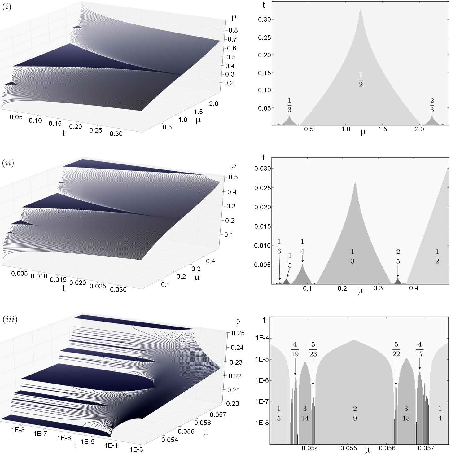
For , each site can accommodate at most one boson and the effective dimension of the local Hilbertspaces reduces to . Figure 3 displays the average ground state densities of the bosons and the localization of the corresponding -phases. To determine the periodicity of the phases we counted the number of eigenvectors of the transfer matrix
| (54) |
with an absolute eigenvalue of one. Once is known follows from the average density. Figure 3 shows a magnification of the area between the -phase and the -phase. The biggest phase between these two phases is the -phase, which can be understood as primary compromise (). In the same fashion we find e.g. that the biggest phase between the phase and is the -phase. The maximal detectable value of is given by the bond dimension of the MPS, which is in case of Figure 3 . However, since the range of covered by the different phases diminishes with growing value of most phases beyond escaped our resolution. The highest value we hit was .
V.1.2 Devils’s Staircase for
For sufficient small the ground states of the Hamiltionian (53) might accommodate more than one boson per site, which allows for new types of Devil’s Staircases. An example is given by Figure 4, which shows the densities and phases for . Here, simple translational invariance is broken by an underlying occupation pattern given by with . Of course, for any non-zero hopping amplitude we expect fluctuations around this pattern such that a more accurate description might be given by , which we need in the next subsection V.1.3. At a certain point, these fluctuations will become so strong that the underlying pattern is destroyed, but this is not the case for the entire region of Figure 4.
In the lobes of the new Devil’s Staircase the sublattice crystallizes in regular pattern of single and double occupied sites. These lobes exhibit an approximate symmetry under the exchange of single and double occupied sites. This is a nontrivial symmetry in contrast to the exact particle hole symmetry of Figure 3 .
Outside the crystalline phases Burnell Burnell et al. (2009) predicted a supersolid like phase. In the following we present numerical evidence which supports this claim.
V.1.3 Supersolids for
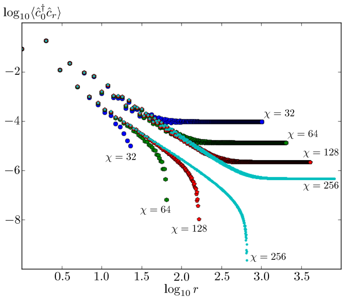
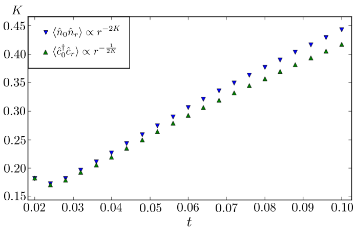
A supersolid is characterized as spatially ordered phase which also exhibits superfluid properties. We already mentioned the spatial order, belonging to Figure 4, which is given by the occupation pattern . In our numerical studies we consider translational invariant superpositions of the ground states, where the occupation pattern is still visible in the two-point correlation functions as and shown in Figure 5 and Figure 6. Due to the spacial order both correlation functions are split into two branches, where correlations belonging to odd distances are strongly suppressed compared to correlations belonging to even distances . Furthermore, both branches exhibit an algebraic decay of the same power. For a superfluide, the power of the decay of is supposed to be reciprocal to the power of . Luttinger liquid theory predicts Giamarchi (2003)
| (55) |
with . These relations are confirmed by our numerical results, as displayed in Figure 7. Both correlation functions give rise to the same Luttinger liquid parameter within a small error range.
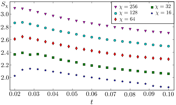
In the thermodynamical limit algebraically decaying correlation functions go hand in hand with an infinite entanglement entropy of the half chain , which can not be represented by any MPS with finite bond dimension . Nonetheless, it was shown Tagliacozzo et al. (2008); Pollmann et al. (2009) that the numerically obtained entropy for such critical phases shows a predictable scaling as function of the MPS bond dimension Pollmann et al. (2009)
| (56) |
where represents the central charge. A demonstration of the scaling behavior is given in Figure 8. From this numerical sample one obtains , which matches drawn from equation (56) for .
VI Conclusion
We have presented several extensions to the basic iMPS algorithm for systems with long-range interactions, some of them with the potential to be useful in a much broader context. A special focus was set on problems arising from broken translational invariance. Here, convergence was ensured by various means, but mainly due to the SMO method which irons out local variations by optimizing exponentially many MPS simultaneously. The new algorithm was successfully applied to calculate detailed Devil’s Staircases and phase diagrams for polar bosons (53) and was also suitable to verify supersolid properties. Theoretical restraints as considered in the comments III.2.2 seem to have negligible influence on practical applications such that the new version of the iMPS algorithm is a genuine improvement in the sense that it can all the old version could plus more.
Acknowledgments
This research was funded by the Austrian Science Fund (FWF): P20748-N16, P24273-N16, SFB F40-FoQus F4012-N16, the European Union (NAMEQUAM) and by the Austrian Ministry of Science BMWF as part of the UniInfrastrukturprogramm of the Research Platform Scientific Computing at the University of Innsbruck. We further like to thank Andrew J. Daley, Marcello Dalmonte, Johannes Schachenmayer, Ulrich Schollwöck and especially Andreas Läuchli for helpful discussions.
Appendix A MPO representation for Hamiltonians
For self-consistency we give a short account based on some examples how to construct an MPO representation for a given Hamiltonian (see also Crosswhite and Bacon (2008); Fröwis et al. (2010); Murg et al. (2010); McCulloch (2007)).
For finite systems with open boundaries the Hamiltonian can be written (4)
First, we need a neat way to write down the explicit form of the fourth order tensors . We write them as matrices whose entries are matrices, too
| (58) |
As an example we consider the Ising Hamiltonian
| (59) |
As we will see below, a possible choice for all in equation (A) with is
| (60) |
and are vectors over matrices
| (61) |
In order to get a better understanding we look at the tensor product of the first tensors. Below (74) we show by induction that
| (63) | ||||
| (65) |
The resulting vector can be seen as an object with three “slots” in which all the relevant information about the first sites are stored. Of course, the number of slots corresponds to the bond dimension of the MPO. The first slot contains all interaction terms between the first sites only and local terms. Since the th site also interacts with the th site, the second slot of the vector passes on and finally, the third slot preserves the identity . For this description is easily checked. The tensor (60) is designed such that it performs the correct induction step
| (70) | ||||
| (72) | ||||
| (74) |
The final tensor is given by
| (75) |
With that we get
| (81) |
We described the vector (65) as an object which contains all relevant information of the sites . This description is true not only for Ising interaction. For any Hamiltonian we have to identify what these relevant information are and design the vector accordingly. As convention, we use the first slot of the vector to store the sum of all interaction terms between the first sites only, including local terms. In the last slot we pass on the identity. The slots in between are needed for interaction terms which involve (at least) one of the first sites and (at least) one of the other sites . In the case of an Heisenberg chain
| (82) |
the vector needs five slots
| (83) |
Further slots might be necessary if we do not restrict ourselves to nearest neighbor interactions.
Once we have identified the structure of , it is straight forward to write the first tensor in vector form. The matrix structure of all the following tensors is constructed column-wise such that the induction
| (84) |
is accomplished as in equation (74) or equation (81) for the final tensor . According to our convention, local terms, as needed in IV.2, are always represented in the bottom left entry of the matrices.
For long-range interaction, the recipe given so far becomes problematic. The longer the range of the interaction, the more information has to be stored in the vector , which usually requires more and more slots. But there are some exceptions (see e.g. Fröwis et al. (2010)). An exponentially decaying interaction needs only one slot – even for infinite range. As an example, we look at the toy Hamiltonian
| (85) |
where is the exponent of and not an index. First, we have to identify the structure of
The crucial observation is, that can be generated iteratively. The following tensors fulfill this task
| (87) | |||||
| (91) | |||||
| (93) |
In order to encode the polynomial decay as into an MPO we resorted to an approximation as a weighted sum of different exponential terms, i.e.
| (94) |
In the appendix of Murg et al. (2010) it is shown how to calculate the optimal and . For the quality of the approximation in dependence of see Crosswhite et al. (2008).
Appendix B Gain function
We like to estimate the influence of in
| (95) |
on which is supposed to minimize . For our numerical purpose the following simple approximation suffices
| (96) |
with = and . The vector is extracted from , which has to be calculated first. This might seem inefficient, since we have to minimize twice – once for and once for the final value of . The solution is to use a minimization routine which projects the minimization onto a small subspace, as explained in section IV.3. This projection has to be done only once but can be used twice. Since the projection is the most time consuming part, the double calculation is done quite cheap. More to this at the end of this subsection.
| (97) | |||||
In the following we approximate . This approximation is not needed but it keeps the calculations clear. In addition, the formula we will derive from the approximated version is numerically more stable. In our program we used the exact version (which we will not derive here) only if .
With , is a parabola in . Assuming that the apex is the minimum one gets
| (98) |
Since for , we choose in accordance with equation (30) to be
| (99) |
From that is calculated to be
| (100) | |||||
B.1 Subspace projection and
As mentioned, we have to solve twice: first for and after that for the final value of . The idea is to reuse the information gathered in the first minimization for the second run. As described in IV.3, the minimization problem is projected onto a subspace. The first basis vector of this subspace is (38). Hence the only element of the subspace matrix (35) which has to be adopted is .
So, the update of the subspace matrix is extremely simple to perform but one might wonder whether the associated basis vectors are still optimal. For the Lanczos Lanczos (1951) and Arnoldi Arnoldi (1951) algorithms, which are built on pure Krylov spaces, it turns out that the influence of on the basis vectors gets extinguished, while for the extended algorithm presented in IV.3 the optimal choice of the basis vectors shows a slight dependence on . Numerically, this is not a serious problem. Nonetheless, since the second optimization is the important one we recommend to use an approximated value of the final to construct the basis vectors in the first run. A simple and effective way is to use from the last tensor optimization assuming . Alternatively, one can solve the intermediate subspace matrices and use these intermediate results to calculate approximations of as described above.
Appendix C Transformation proof for degenerate ground states
Let and represent two different ground states to the same Hamiltonian with a times degenerate ground state level due to broken translational invariance
| (101) |
If degenerations due to further symmetries are involved, and are supposed to have the same characteristic values for these symmetries. This allows us to operate as if no further symmetries exist, since all operations we are about to use leave these characteristic values unchanged. Under this condition we will prove the existence of a matrix such that the ground state can be expressed using the tensors stemming from the iMPS
| (102) |
where .
Let us start by surveying the elements of the proof. In order to show the claimed equation (102) we will actually prove the gauge transformation
| (103) |
This gauge transformation will be proven for the case that the two underlying MPS represent the same physical state – which is not given for and (101). In order to use the gauge proof for our purpose we need to find one physical state described by two different MPS where the first MPS be constructed using the of and the second by the of . This one state which allows us to complete our proof is the translational invariant ground state. According to our preliminary remarks this state is unique. Hence, if we succeed to construct two different MPS which represent a translational invariant ground state, we know that they represent the same physical state as demanded. We will prove the following construction for this state
| (104) | |||||
with new tensors and .
We start by showing the gauge transformation (103). In order to increase clarity we define
| (105) |
For this specific gauge proof the different do not need to be of the same structure and neither do the . But in contrast to the the still have to fulfill equation (9), i.e.,
| (106) | |||||
Although not an identity, the operator acts like such if it is applied from the left on any MPS with the structure , where represents an arbitrary right side of the MPS. Using the identity (106) we get
| (107) |
In the following we assume that the two MPS
| (108) |
represent the same physical state. Now, let us apply the operator on this equation. Due to equation (107) the left side stays unchanged. Hence the physical state represented by the right side does not change either
| (109) |
with . The existence of the inverse with can be assured: if the rank of is smaller than the bond dimension , the value of can be reduced, since in that case it turns out to be unnecessarily high. Applying from the right on equation (109) we end up with
| (110) |
For this covers the first part of the heralded gauge equation (103). The second part of equation (103) is proved by a straight forward application of the arguments used above on the right side of the MPS.
Now, we have to show the MPS construction of the translational invariant ground state (104). As above, we assume that the ground state level of the Hamiltonian under consideration is times degenerate due to broken translational invariance. Let be the operator which shifts all sites of an MPS by one position to the left and . For the MPS representing any of the possible ground states we get
| (111) |
where represents an unnormalized version of the translational invariant ground state, which we like to construct. As an intermediate step we like to prove equation (115) below. Therefor we have to look at the effect has on (using equation (101) for )
| (112) |
Next, we look at the MPS , which has the form
| (113) |
Since the two MPS describe the same physical state we are allowed to apply the gauge transformation (110) and identify
| (114) |
Inserting this expression into equation (112) we arrive at the following description for
| (115) |
As we see, applying the operator on has the same effect as the replacement of the matrix by . Since higher powers of can be created by an iteration of the arguments just presented, it follows that the effect of any on can be accounted for by an accordingly calculated . Following that construction the only difference between the various MPS is their tensor and hence the task of equation (111) to sum up these MPS reduces to a summation of the . In other words: Replacing the matrix in the MPS by
| (116) |
results in the translational invariant MPS . Of course, the same arguments can be applied to the MPS giving us as claimed in equation (104).
Let us review our arguments: By virtue of equation (116) we can transform the MPS and given in equation (101) such that we end up with the translational invariant ground state and as claimed in equation (104). Since we work under the condition that we are allowed to use the gauge transformation (110) to replace the of by the of . The same replacement is possible in because the in and are identical (as are the in and ). This concludes the proof of equation (102) we aimed for.
Appendix D Davidson implementation
In this subsection we introduce a practical implementation resembling the Davidson Sleijpen and Van der Vorst (2000) method based on recycled information of the previous round, which allows to improve the update equation (37) of the iterative eigenvector solver presented in section IV.3. We adopt the same notation as in that section but mostly drop the index to keep the formulae clean.
The best possible new vector the iterative eigenvector solver could come up with to replace equation (37) is an orthonormalized version of .
| (117) |
where we used the definition (36) for . The Davidson method requires a workable approximation for the non trivial operator . At this point we take advantage of the expectation that the operator calculated in round should look pretty much the same as calculated in round
| (118) |
Hence we use the accumulated data at the end of round for an efficient one time estimation of , which we will apply in round .
In order to calculate we need a simplified form of which allows easy inversion. We know approximated eigenvectors of . In order to have an orthonormal basis for we imagine further , where . With that we approximate as
| (119) | |||||
with an average eigenvalue for the unknown eigenvectors. One might be tempted to simplify equation (119) using – but we do not, since the eigenvectors are not very well approximated except for . To be able to perform the inversion in equation (122) it suffices to resort to the exact result
| (120) |
which is a consequence of the construction (35). Further, with the results gathered during the optimization (IV.3) the are as quickly calculated as the .
Next, we take the trace of equation (119) and set such that both sides are equal
| (121) |
The trace of the exact is efficiently calculated by already tracing over its components and before assembling them (15).
Now we insert the approximated (119) in
| (122) | |||||
The inversion is solved by
| (123) |
as can be verified inserting the result in .
The final question we have to answer is which value we assign to the unknown exact eigenvalue . The best approximation (which we already used in equation (117)) is , but this produces a singularity in . There are two ways out. First, we can always pick a little bit lower . Second, we should discard the troublesome term in anyway for the following reason: We replace equation (37) by
| (124) |
where and with that . Afterwards, residual parts of the term are exfiltrated again because has to be orthogonalized (and normalized)
| (125) |
These considerations are also part of the more elaborated Jacobi-Davidson Sleijpen and Van der Vorst (2000) method to which this implementation can be extended.
We might further consider to omit terms with since their influence shrinks with . At the end of the day, the effort to construct as well as the effort for each application scale with times the number of terms used in .
Appendix E Altered minimization
Here we derive the missing equations of III.4. First, we search for an approximation of and start by an alternative way of expressing them
| (126) |
where we used the orthogonality (9) of the and the decomposition (8). Next, we use the fact that the algorithm is tuned to produce consecutive tensors which are quite similar. Hence we approximate the yet unknown (126) by their known predecessor of the optimization round before, i.e. .
| (127) |
Appendix F Mirror symmetry
Here we show that in case of a mirror symmetric Hamiltonian i.e. a Hamiltonian that is invariant under inversion of the order of its sites
| (131) |
all tensors can be chosen mirror symmetrical in their auxiliary indices , i.e.
| (132) |
This allows to impose an extra constraint on . Commuting the indices also results in
| (133) |
as can be seen directly from the decomposition (8). Further it is possible to construct and (19) such that they are identical. But therefor we need to resort to an alternative MPO construction for the Hamiltonian, such that the MPO tensors of the left half are mirror symmetric to the tensors of the right half. This can be achieved if we include a special interface tensor in the middle where and are connected to build . This reduces the requirement in storage memory roughly by a factor of 2, but has nearly no effect on the speed. Since storage capacities are usually not a big issue, we do not elaborate this point any further.
One should be aware that equation (131) enforces a mirror symmetric MPS. In case of a mirror symmetry breaking ground state, the MPS will represent a superposition of both chiralities, implying an unfavorably increased requirement in bond dimension.
We further remark that our definition of a mirror symmetric Hamiltonian does not forcedly imply a symmetry in real space. Although in practical application the order of the sites generally coincides with one specific spatial direction, there is no mathematical connection between the direction of space and the chosen order.
Assuming a mirror symmetric Hamiltonian (131) the claim of the mirror symmetric tensor (132) can be proven iteratively:
The very first is constructed via the initialization procedure described in II.5.2. If we start with a mirror symmetric wave function and use Takagi’s factorization as suggested in 3. of the initialization procedure, is symmetric and the induction is well grounded.
Proof for 1. All represent a sum of operators according to equation (18)
| (134) |
Each of these contains an entire Hamiltonian MPO as central unit sandwiched by bra and ket MPS, with a hole where the new tensor is supposed to be inserted. The Hamiltonian is guaranteed to be mirror symmetric, while there is no such condition for the MPS. The different MPS are encoded in the building blocks and , which are constructed symmetrically (19), i.e., in contrast to the basic algorithm each new tensor is inserted in and at equal footing. Hence, for each MPS exists a counterpart which contains exactly the same tensors in inverted order. In general, this alone is not enough, because mirror symmetry also exchanges the left and right auxiliary indices. But, since all involved tensors are supposed to be invariant under this kind of exchange (and (133), as needed), mirror symmetric counterparts for all involved MPS are guaranteed and with that is mirror symmetric.
Proof for 2. The tensor is the result of the minimization procedure described in more details in IV.3. Each element in this procedure maintains mirror symmetry if and the initial tensor (27) are mirror symmetric. Since is a superposition of mirror symmetric tensors, all conditions are met.
Finally we remark that accumulating numerical errors might undermine the symmetry. Therefore we recommend to explicitly restore the symmetry of each during its calculation.
References
- Schollwoeck (2011) U. Schollwoeck, Annals of Physics 326, 96 (2011).
- White (1992) S. R. White, Phys. Rev. Lett 69, 2863 (1992).
- Fannes et al. (1992) M. Fannes, B. Nachtergaele, and R. F. Werner, Comm. Math. Phys. 144, 443 (1992).
- Affleck et al. (1987) I. Affleck, T. Kennedy, E. H. Lieb, and H. Tasaki, Phys. Rev. Lett. 59, 799 (1987).
- Dukelsky et al. (1998) J. Dukelsky, M. A. Martín-delgado, T. Nishino, and G. Sierra, Europhys. Lett. 43, 457 (1998).
- Vidal (2007a) G. Vidal, Phys. Rev. Lett. 99, 220405 (2007a).
- Hübener et al. (2009) R. Hübener, C. Kruszynska, L. Hartmann, W. Dür, F. Verstraete, J. Eisert, and M. Plenio, Phys. Rev. A 79, 022317 (2009).
- Hübener et al. (2010) R. Hübener, V. Nebendahl, and W. Dür, New J. Phys. 12, 025004 (2010).
- Eisert (2006) J. Eisert, Phys. Rev. Lett. 97, 260501 (2006).
- Schuch et al. (2008) N. Schuch, I. Cirac, and F. Verstraete, Phys. Rev. Lett. 100, 250501 (2008).
- Burnell et al. (2009) F. J. Burnell, M. M. Parish, N. R. Cooper, and S. L. Sondhi, Phys. Rev. B 80, 174519 (2009).
- Schachenmayer et al. (2010) J. Schachenmayer, I. Lesanovsky, A. Micheli, and A. J. Daley, New J. Phys. 12, 103044 (2010).
- Trefzger et al. (2011) C. Trefzger, C. Menotti, B. Capogrosso-Sansone, and M. Lewenstein, J. Phys. B: At. Mol. Opt. Phys. 44, 193001 (2011).
- Cardy (1996) J. Cardy, Scaling and renormalization in statistical physics (Cambridge University Press, 1996).
- Pirvu et al. (2012) B. Pirvu, G. Vidal, F. Verstraete, and L. Tagliacozzo, Phys. Rev. B 86, 075117 (2012).
- Gendiar et al. (2011) A. Gendiar, M. Daniska, Y. Lee, and T. Nishino, Phys. Rev. A 83, 052118 (2011).
- Vidal (2007b) G. Vidal, Phys. Rev. Lett. 98, 070201 (2007b).
- McCulloch (2007) I. P. McCulloch, J. Stat. Mech. , 10014 (2007).
- Murg et al. (2010) V. Murg, J. Cirac, B. Pirvu, and F. Verstraete, New J. Phys. 12, 025012 (2010).
- Crosswhite and Bacon (2008) G. M. Crosswhite and D. Bacon, Phys. Rev. A 78, 012356 (2008).
- Fröwis et al. (2010) F. Fröwis, V. Nebendahl, and W. Dür, Phys. Rev. A 81, 062337 (2010).
- Crosswhite et al. (2008) G. M. Crosswhite, A. C. Doherty, and G. Vidal, Phys. Rev. B 78, 035116 (2008).
- (23) I. P. McCulloch, E-print: arXiv:0804.2509v1.
- Sleijpen and Van der Vorst (2000) G. L. G. Sleijpen and H. A. Van der Vorst, SIAM Review 42, 267 (2000).
- Hastings (2007) M. B. Hastings, JSTAT , 08024 (2007).
- Ueda et al. (2011) H. Ueda, I. Maruyama, and K. Okunishi, J. Phys. Soc. Jpn. 80, 023001 (2011).
- Ueda and Maruyama (2012) H. Ueda and I. Maruyama, E-print: arXiv:1112.2075v2 (2012).
- Saad (2003) Y. Saad, Iterative methods for sparse linear systems (2nd ed.) (SIAM. ISBN 0898715342, 2003).
- Lanczos (1951) C. Lanczos, Journal of research of the National Bureau of Standards 45, 255 (1951).
- Arnoldi (1951) W. Arnoldi, Quarterly of Applied Mathematics 9, 17 (1951).
- Furukawa et al. (2012) S. Furukawa, M. Sato, S. Onoda, and A. Furusaki, Phys. Rev. B. 86, 094417 (2012).
- Okunishi (2008) K. Okunishi, J. Phys. Soc. Jpn. 77, 114004 (2008).
- (33) F. J. Burnell, E-print: arXiv:1004.5595v2.
- Bak and Bruinsma (1982) P. Bak and R. Bruinsma, Phys. Rev. Lett. 49, 249 (1982).
- Giamarchi (2003) T. Giamarchi, Quantum Physics in One Dimension (Oxford University Press, 2003).
- Tagliacozzo et al. (2008) L. Tagliacozzo, T. R. de Oliveira, S. Iblisdir, and J. I. Latorre, Phys. Rev. B 78, 024410 (2008).
- Pollmann et al. (2009) F. Pollmann, S. Mukerjee, A. M. Turner, and J. E. Moore, Phys. Rev. Lett. 102, 255701 (2009).