Virial expansion coefficients in the harmonic approximation

Abstract

The virial expansion method is applied within a harmonic approximation to an interacting $N$-body system of identical fermions. We compute the canonical partition functions for two and three particles to get the two lowest orders in the expansion. The energy spectrum is carefully interpolated to reproduce ground state properties at low temperature and the non-interacting large temperature limit of constant virial coefficients. This resembles the smearing of shell effects in finite systems with increasing temperature. Numerical results are discussed for the second and third virial coefficients as function of dimension, temperature, interaction, and the transition temperature between low and high energy limits.

I Introduction

The virial expansion is a classical concept thie85 ; onne01 ; urse27 ; hill56 which has been extended to be applicable for quantum mechanical systems kahn38 . The expansion is in terms of few-body correlations and therefore most efficient when the influence of $N$-body effects decrease with $N$. In practice, this decrease has to be very fast, because higher order correlations are extremely difficult to obtain by accurate calculations. This fact is not obvious since only the spectrum of $N$ interacting particles is needed, not wave functions or structure nor any other properties. However, obtaining these spectra imply solving the $N$-body problem which is already demanding beyond two particles for general interactions.

In the classical textbook by Huang on statistical mechanics huang87 , the virial expansion is discussed for the quantum mechanical case and it is elegantly demonstrated how the second virial coefficient can be obtained from knowledge of the two-body scattering phase shift and bound state spectrum (when present). This was subsequently generalized in the seminal paper of Dashen, Ma, and Bernstein dashen1969 where a formulation of statistical mechanics in terms of the scattering $S$-matrix is given. The formulation gives a prescription for calculating virial coefficients at any order, and shortly thereafter the behavior of the third order coefficient at low temperature was obtained via the $S$-matrix method adhikari1971 . The $S$-matrix approach to virial coefficients is still an actively research topic how2010 with recent applications in the field of cold atomic gases leclair2012 . However, since determining the $S$-matrix in a general system with multiple particles is a high non-trivial task, it is valuable to pursue alternative ways of approaching the virial expansion.

Approximations or assumptions are unavoidable at some point. The traditional strategies have been either to limit the Hilbert space allowed for the variational many-body wave functions or to design schematic Hamiltonians aiming for specific features. The latter approach requires great care and physical intuition to retain the necessary features of the Hamiltonian that will accurately describe the phenomena under study. An approach along this second line of reasoning is the use of harmonic Hamiltonians where interaction terms are replaced by harmonic oscillators. This is extremely convenient from a computational point of view as many aspects become analytically addressable for both fermionic and bosonic systems brosens97 ; magda00 ; brosens ; tempere .

The replacement of one- and two-body terms in the Hamiltonian by harmonic forms leaves the problem of determining the parameters of the harmonic Hamiltonian according to given criteria. Here one must again take guidance from physical properties and aspects of the system that are crucial for the system under study. Recently, we formulated an approach that explores the $N$-body problem in an external parabolic confining potential by fixing the two-body interactions to the properties of an exactly solvable problem in the same geometry arm11 . The two-body information needed is the energy eigenvalues and structural properties of the wave function such as radial averages.

The example studied in Ref. arm11 was short-range interacting particles in a harmonic trap for which the two-body problem can be exactly solved in the zero-range limit busc98 . Within the field of cold atomic gases, this solution was subsequently confirmed by different experimental groups stoferle06 . The model studied in Ref. busc98 has since been used as a starting point in both nuclear and cold atomic gas physics haxton02 . Recently, the harmonic approximation with parameters fixed to exact two-body properties have been applied to particles that interact via dipole forces arm10 ; vol12a ; dip12 ; wang06 ; pikovski11 and shown to accurately reproduce numerical few-body results for moderate-to-strong dipole strengths shih09 ; klawunn10 ; baranov11 ; vol11 .

This harmonic method has also been extended to the thermodynamical regime at finite temperature magda00 ; brosens97 ; arm12a , where it has been shown using a path-integral formalism that the canonical partition function for given particle number can be obtained brosens97 ; lemmens1999 ; tempere ; klimin2004 ; brosens2005 . Here we consider an alternative approach that uses exact diagonalization of the Hamiltonian and subsequent calculation of the relevant degeneracies in the energy spectrum for a given number of particles arm12a . This is in contrast to the usual approximation using the grand partition function where only the average particle number is conserved. The method applies to both identical bosons and fermions as well as distinguishable particles and combinations of all these possibilities arm11 ; arm12a ; vol12a . The difficult part is to find the degeneracies of the $N$-body spectrum for the specified symmetries required by quantum statistics. The energies themselves are easily found from the harmonic oscillator solutions.

Here we consider the virial expansion within the harmonic Hamiltonian approximation for identical fermions. This paper is a natural extension of Ref. arm12a where the thermodynamics of small to moderate size systems of fermions and bosons was considered by direct computation of the partition function. This requires a numerically efficient determination of the level degeneracies which is, however, only possible up to moderate particle numbers ($N\sim 20$) even in a harmonic model. The virial expansion is usually a rapidly converging series and we therefore expect to be able to compute coefficients within the harmonic approach. However, there are some subtleties with the convergence of the coefficients that must be carefully handled. Therefore we focus almost exclusively on the formal development of the virial expansion within the harmonic approximation.

A motivation for our work is the recent investigation of universal thermodynamics within cold atomic gas experiments ufermi where the virial expansion has been succesfully applied virial . However, the expansion is general and is applicable to other fermionic systems. While the typical condensed-matter and cold atom fermion systems have two internal (spin or hyperfine spin) components, we consider the case of single-component fermions here in order to keep the formalism simple while still retaining the full quantum statistical properties of a Fermi system. Multi-component fermionic and bosonic systems will be considered in subsequent studies.

The purpose of the present paper is to formulate and explore the harmonic method and the virial expansion to prepare for future applications to systems in both cold atomic gases, nuclear physics, as well as condensed-matter systems. The paper is organized as follows; We describe the ingredients of the method in Sec. II The numerical illustrations follow in Sec. III for the lowest virial coefficients. In Sec. IV we summarize and provide an outlook for future directions of interest.

II Theoretical description

We first present general definitions of the crucial ingredients. Then we apply the formulation to the results of a system of $N$ particles described by a coupled set of harmonic oscillator potentials. The approach to the large temperature limit is finally modified to exhibit the behavior corresponding to the correct high energy spectrum.

II.1 Basic definitions

The classical virial expansion is an expansion of the equation of state of a gas of identical particles, usually in powers of the number density $\rho$, see e.g. thie85 ; onne01 ; urse27 ; hill56 :

$$p=k_{B}T\rho(1+B_{2}(T)\rho+B_{3}(T)\rho^{2}+\dots),$$ (1)

where $p$ is the pressure, $k_{B}$ is Boltzmann’s constant, $T$ is the temperature, and the $B_{i}$’s are the virial coefficients of the expansion. In the classical expansion, they are related to the intermolecular or interatomic potentials of $i$ interacting particles. The advantage of the expansion is that it reveals deviations from ideal gas behavior by examining just the few-body aspects of the system. The leading term is then the ordinary ideal gas expression for a non-interacting system. The second term in the classical expansion in three dimensions is given by the $B_{2}$-coefficient

$$B_{2}=-\frac{1}{2}\int[\exp(-\beta V_{12}(r))-1]d^{3}r,$$ (2)

where $V_{12}$ is the inter-particle potential depending on the relative coordinate $r$, and $\beta=1/k_{B}T$. The integral in Eq. (2) is known as a configuration integral, and from it one can see that this coefficient only converges for potentials which decay faster than $1/r^{3}$. The convergence in two dimensions is correspondingly only achieved when $V$ decays faster than $1/r^{2}$. The general coefficient is

$$B_{i} = -\frac{i-1}{i!V}$$

$$\sum\textrm{(all independent i-cluster integrals)},$$

where $V$ is the volume of the system. The i-cluster integrals are all the independent clusters containing the i-particles, first presented graphically by maye40 . A cluster in this context can be visualized graphically by thinking of $i$ numbered circles with lines connecting them symbolizing the interaction between those particles. These lines can be drawn in many different ways, the only requirement for the $i$-cluster is that all $i$ atoms or molecules must be connected to at least one other member of the system. The quantum mechanical version of the cluster expansion was developed at around the same time by kahn38 .

For a system of quantum mechanical particles with Fermi or Bose statistics, the expansion is most commonly performed in the fugacity, $z=\exp{(\beta\mu)}$, of the system, where $\mu$ is the chemical potential of the $N$-body system. The grand canonical partition function, $\mathcal{Z}$, is written as an expansion in $z$

$$\mathcal{Z}=1+zQ_{1}+z^{2}Q_{2}+\dots,$$ (4)

which translates into an expansion for the grand thermodynamic potential, $\Omega$:

$$\Omega=-k_{B}TQ_{1}[z+b_{2}z^{2}+b_{3}z^{3}+\dots].$$ (5)

The first virial coefficients can explicitly be written:

$$b_{2} = (Q_{2}-Q_{1}^{2})/Q_{1}$$ (6)

$$b_{3} = (Q_{3}-Q_{1}Q_{2}+Q_{1}^{3}/3)/Q_{1}$$ (7)

$$b_{4} = (Q_{4}-Q_{1}Q_{3}+Q_{1}^{2}Q_{2}+Q_{2}^{2}/2-Q_{1}^{4}/4)/Q_{1}\;,$$ (8)

where $Q_{N}$ is the canonical partition function for $N$ particles of the proper symmetry, that is

$$Q_{N}=\sum_{j}g_{j}^{(N)}\exp(-\beta E_{j}^{(N)})\;,$$ (9)

where $g_{j}^{(N)}$ and $E_{j}^{(N)}$ are the degeneracy and energy of the $j$’th state of the $N$-body system. Thus $Q_{N}$ can be calculated solely from the energy spectrum of the $N$-body system, and all thermodynamic quantities can then be obtained from $\Omega$ in Eq. (5) to the order desired. The classical virial expansion, Eq. (1), can be recovered from the quantum version introduced above by using $\langle N\rangle=-\tfrac{\partial\Omega}{\partial\mu}|_{\textrm{T,V}}$ and $\Omega=-pV$ (see for instance Ref. reichl1998 where the relation of $B_{i}$ and $b_{i}$ is also discussed). In the present case we have an external trap and the volume must be suitable translated into parameters of the trap before making detailed comparisons to experiments or other studies hu2010 .

In practical calculations, it is more convenient to consider the difference between interacting and non-interacting systems. We then consider the differences $\Delta Q_{n}=Q_{n}-Q_{n}^{(1)}$ and $\Delta b_{n}=b_{n}-b_{n}^{(1)}$, where the superscript (1) denotes a non-interacting system having the same $N$-body fugacity $z$. We can then re-write Eq. (5) as

$$\Omega=\Omega^{(1)}-k_{B}TQ_{1}[\Delta b_{2}z^{2}+\Delta b_{3}z^{3}+\dots]\;,$$ (10)

where $\Omega^{(1)}$ is the grand thermodynamic potential of the non-interaction system with the same fugacity. The differences of the virial coefficients in Eqs. (6)-(8) become

$$\Delta b_{2} = \Delta Q_{2}/Q_{1}$$ (11)

$$\Delta b_{3} = \Delta Q_{3}/Q_{1}-\Delta Q_{2}$$ (12)

$$\Delta b_{4} = \Delta Q_{4}/Q_{1}-\Delta Q_{3}+Q_{1}\Delta Q_{2}$$ (13)

$$+ (Q_{2}^{2}-(Q_{2}^{(1)})^{2})/(2Q_{1})\;.$$

These definitions and expressions are general and now applicable to a specified set of potentials producing the partition functions $Q_{n}$ and the corresponding (differences of) virial coefficients.

II.2 Harmonic approximation

The one- and two-body interactions for the $N$-body system are approximated by second order polynomials in Cartesian coordinates. The Hamiltonian is a sum of similar terms from each spatial dimension, $H=H_{x}+H_{y}+H_{z}$. In the present work we consider the two- and three-dimensional cases. For identical particles of mass $m$ the Hamiltonian of the $x$-direction is

$$H_{x} = -\frac{\hbar^{2}}{2m}\sum_{k=1}^{N}\frac{\partial^{2}}{\partial x_{k}^{2}}+e\frac{1}{8}m\omega_{in}^{2}\sum_{i,k=1}^{N}(x_{i}-x_{k})^{2}$$ (14)

$$+\frac{1}{2}m\omega_{0}^{2}\sum_{k=1}^{N}x_{k}^{2}+\frac{N(N-1)}{2}V_{sx}\;,$$

where $x_{i}$ is the coordinate of particle $i$, $\omega_{0}$ and $\omega_{in}$ are frequencies of the one and two-body interactions, and $V_{sx}$ is a constant adjusting the energy to the desired value. The factor 1/8 in the second term comes from the use of the reduced mass equal to $m/2$ and to avoid double counting in the sum.

The frequencies and the constant shift can be chosen to reproduce certain properties of a modeled system as discussed in arm11 . How these parameters are chosen does not affect the computation of the virial coefficients which therefore are obtained as functions of the parameters in the Hamiltonian. The method is general and applicable as soon as a Hamiltonian of the oscillator form is available. It is, however, still useful to illustrate by describing the procedure for a specific system. We focus on a system of identical, spin-polarized fermions confined in an external trap arm11 where the fermions interact via a short-range potential. Due to the Pauli principle, the particles cannot interact in the spherical $s$-wave channel, and the lowest non-trivial interaction will be odd and of the $p$-wave kind (higher odd partial wave channels will be neglected). In the zero-range limit, the model of Busch et al. busc98 can still be solved for $p$-wave interactions in both three- pwave3D and two-dimensional pwave2D traps. We adjust the interacting frequency, $\omega_{in}$, to reproduce some property related to the spatial extension of the correct two-body wave function (the average square radius in the two-body ground state in the trap). The shift, $V_{sx}$, is then added to make sure that the exact two-body ground state energy is reproduced by the oscillator potential. Notice that this (constant) energy shift does not influence thermodynamics in any essential way. We therefore ignore it for most of our discussion except for some comments near the end of Sec. III.

The accuracy of the harmonic approximation should depend on the degree to which the physical two-body potential allows a quadratic expansion. Naively, this should be the case for potentials that have a sizable attractive pocket, which is true for many molecular potentials that allow a large number of bound states peder2012 . An example is the Morse potential which has been explored in the harmonic approximation in Ref. tempere . As mentioned in the introduction, for dipolar particles, the harmonic approximation is extremely accurate, even in the regime of small dipole moments when suitable adjustment of the harmonic frequency is performed arm10 ; vol12a ; dip12 . In fact, even when the real potential is shallow, the energy can be reproduced to a few percent accuracy with a careful choice of gaussian wave function as shown in Ref. dip12 .

For typical cold atomic gas setups, one has harmonically trapped atoms interacting via short-ranged interactions. In the idealized limit of zero-range interactions, the two-body problem is exactly solvable as demonstrated by Busch et al. busc98 . In Ref. arm11 , the exact solution was used to fit the oscillator parameters that provide the input for the harmonic approximation. In the strongly-bound limit where a deep two-body bound state occurs, this choice of parameters leads to the same scaling of the energy with particle number that is observed in variational approaches variational ; fu2003 . Also, when the interactions have a diverging two-body scattering length (the unitarity limit), the two-body wave function becomes similar to the non-interacting wave function in the trap busc98 and we therefore expect the harmonic approximation to be very good. These features are clearly seen in the one-dimensional case as discussed in Ref. jeremy2012 . As discussed in Ref. busc98 , the one- and three-dimensional cases are very similar. The scalings away from these limiting cases are similar but not identical to other approaches. In general, we expect the harmonic approximation to give good qualitative results for strong interactions, but do not expect perfect quantitative agreement with variation or numerics. On the quantitative side, we note that for one-dimensional systems, the three-body energy can be reproduced to within 10 percent in the strongly-bound limit jeremy2012 . We thus estimate similar accuracy on the third virial coefficient. At this point we leave the question of how to adjust the two-body parameters of the Hamiltonian and proceed with a general discussion for arbitrary parameters.

The solution to Eq. (14) is found by a coordinate transformation which splits the Hamiltonian into $N$ independent harmonic oscillators with new coordinates and frequencies related to the normal modes of the $N$-body system. For $N$ identical particles two new normal mode frequencies are produced, that is the external trap frequency, $\omega_{0}$, corresponding to the center of mass motion, and the $N-1$ times degenerate frequency, $\omega_{r}$, given by

$$\omega_{r}^{2}=N\omega_{in}^{2}/2+\omega_{0}^{2}\;.$$ (15)

The degenerate frequencies correspond to different types of intrinsic (relative) motion which for two particles is simply oscillations in the relative coordinate, but in the general case correspond to different normal modes of the system. The $N$-body energy spectrum is

$$E_{j}=E_{cm}+E_{rel}+V_{S},V_{S}=\frac{D}{2}N(N-1)V_{sx},$$ (16)

$$E_{cm}=\hbar\omega_{0}\left(n_{0}(j)+\frac{D}{2}\right),n_{0}(j)=\sum_{i=1}^{D}n_{0,i}(j),$$ (17)

$$E_{rel}=\hbar\omega_{r}(n_{r}(j)+\frac{D}{2}(N-1))+V_{S},$$ (18)

$$n_{r}(j)=\sum_{i=1}^{D}\sum_{k=1}^{N-1}n_{k,i}(j)=\sum_{i=1}^{D}n_{r,i}(j),$$ (19)

where $j$ is the index of the $N$-body states. $n_{0,i}$ is the number of excitation quanta in the center-of-mass degree of freedom in the $i$’th direction, while $n_{k,i}$ is the number of quanta in the $k$’th of the $N-1$ degenerate $\omega_{r}$ modes in the $i$’th direction. The energy state $j$ is thus given by specifying the number of excitation quanta in each normal mode for all dimensions. Here we have divided into center of mass and relative contributions since in the equal mass case studied here these can be separated completely.

II.3 The lowest virial coefficients

The partition function for one particle, $Q_{1}$, is the trivial problem of one particle in an external harmonic trap of $D$ dimension. Since it has no other particles to interact with, the spectrum arises only from center of mass motion for one particle. The partition function is in this case found from Eqs. (9) and (17) to be

$$Q_{1}=\left(\frac{\exp(-\Theta_{0}/(2T))}{1-\exp(-\Theta_{0}/T)}\right)^{D}=\frac{1}{2^{D}}\sinh^{-D}\big{(}\frac{\Theta_{0}}{2T}\big{)}\;,$$ (20)

where $\Theta_{0}=\hbar\omega_{0}/k_{B}$.

The partition function for two particles, $Q_{2}$, is found from Eqs. (9), (16), (17), and (18), and can be factorized into center of mass and relative contributions. The center of mass piece is completely symmetric in all the coordinates, so it plays no role in determining the overall symmetry of the system. It is just a geometric series in $D$ dimensions, and in fact equal to $Q_{1}$, since the frequency is that of the external trap.

The relative motion corresponds to the difference between the two individual coordinates. For fermions this motion then must provide the antisymmetry of the wave function corresponding to an odd number of relative oscillator quanta, $n_{r}(j)$, in Eq. (18). The energies are completely specified by the quanta and the related degeneracy is easily counted for the relative motion of two particles. To obtain an analytical, closed solution, it is convenient to consider the individual Cartesian quanta. In 2D, one merely needs to keep either quanta, $n_{r,x}$ or $n_{r,y}$ odd in $x$ or in $y$-directions. In 3D, there are two possiblities, in that all three quanta are odd or two are even and one is odd. With these restrictions the summation in Eq. (9) leads for $D=2$ to

$$Q_{2}=Q_{1}\left(\frac{\exp(-\Theta_{r}/T)}{1-\exp(-2\Theta_{r}/T)}\right)^{2}\exp(-\Theta_{S}/T)\,,$$ (21)

where $\Theta_{S}=V_{S}/k_{B}$ and $\Theta_{r}=\hbar\omega_{r}/k_{B}$. For $D=3$, we find instead

$$Q_{2} = Q_{1}\exp(-\Theta_{S}/T)$$

$$\times\frac{3\exp(-5\Theta_{r}/(2T))+\exp(-9\Theta_{r}/(2T))}{[1-\exp(-2\Theta_{r}/T)]^{3}}$$

The next terms involve the partition function, $Q_{3}$, for the three-body system. A completely closed form solution for the partition function is not found, and we keep the expression as an energy sum over three-body states. The center of mass summation is again performed analytically, and Eqs. (16) and (18) lead to the other factors amounting in total to

$$Q_{3}=Q_{1}\exp(-\Theta_{S}/T)\sum_{l=0}^{\infty}g_{l}\exp(-(l+D)\Theta_{r}/T)\;,$$ (23)

where the summation over all states is reduced to run over all integers. The difficulty is then only to know the corresponding degeneracy, $g_{l}$. This number of states of a given excitation energy is found by the method described in arm12a . The expression in Eq. (23) is formally the same in two and three dimensions but the degeneracy factors differ substantially. The infinite sum must in practice be truncated at some level of excitation. Ideally this is after convergence is reached. However, this depends strongly on the value of the temperature and we therefore first must decide how large $T$-values we need to investigate.

The differences between interacting and non-interacting virial coefficients are found from Eqs. (11) and (12). The non-interacting partition functions are structurally the same as the interacting ones, only with $\Theta_{r}$ replaced by $\Theta_{0}$, and $\Theta_{S}=0$. Using the expressions in Eqs. (21), (II.3), and (23), we can therefore easily find $\Delta b_{2}$ and $\Delta b_{3}$. For $\Delta b_{2}$ in two dimensions we explicitly get

$$\Delta b_{2} = \exp(-\Theta_{S}/T)\left(\frac{\exp(-\Theta_{r}/T)}{1-\exp(-2\Theta_{r}/T)}\right)^{2}$$ (24)

$$-\left(\frac{\exp(-\Theta_{0}/T)}{1-\exp(-2\Theta_{0}/T)}\right)^{2}\,,$$

and a slightly more complicated expression for three dimensions from Eq. (II.3). In the same way we can of course re-write $\Delta b_{3}$ in terms of the expression for $Q_{3}$ in Eq. (23), but due to the lack of closed form it does not provide any further information.

Notice that the low-temperature limit of the virial coefficients above is determined by the value of the shift, $\Theta_{S}$. From Eq. (24) we see that $\Delta b_{2}$ will vanish for $T\to 0$ whenever we have $\Theta_{S}+2\Theta_{r}>0$, similarly for the higher virial coefficients. In the following we will mostly discuss the case $\Theta_{S}=0$, i.e. no shift at all, since this is the relevant case for thermodynamics. For generality, we comment briefly on the influence of the shift for all temperatures in Sec. III.

II.4 Large-temperature limits

At high temperature, the interacting system should approach a non-interacting system as the kinetic energy dominates the potential. This does not imply that all $\Delta b_{i}$ must vanish at large $T$, since deviations in the low-energy spectrum between interacting and non-interacting systems easily produce different large-temperature contributions. This can be seen by dividing the sum over states in the partition functions in low- and high-energy parts. Even if we assume that the high-energy interacting and non-interacting spectra become equal and would thus not contribute to $\Delta b_{i}$, the low-energy parts remains different and this yields a contribution to the virial coefficient for all temperatures. However, such difference must remain finite since it arises from a finite energy interval.

As stated before, the virial expansion does not work for potentials that do not vanish at a fast enough rate, so one would think that the harmonic potential, which does not vanish at all, would cause problems. Indeed, if we use the derived expressions all our $\Delta b_{i}$ diverge with increasing temperature. The origin of this problem is simply that the energy spectrum is obtained for the $N$-body solution of a temperature independent Hamiltonian adjusted to reproduce ground state properties. This does not account for the influence of temperature on the effective interactions and, in turn, on the energy spectrum. This may also be expressed in terms of an excitation energy dependence of the effective interaction as seen for example in the variation of the mean-free-path. Since excitation energy on average can be related to temperature these formulations are equivalent.

To pin-point the problem and subsequently cure it we start with $\Delta b_{2}$. In the limit of high temperature, Eq. (24) can be expanded to leading orders in $T$ to give

$$\Delta b_{2}(T\to\infty)=T^{2}\left(\frac{1}{4\Theta_{r}^{2}}-\frac{1}{4\Theta_{0}^{2}}\right)-T\frac{\Theta_{S}}{4\Theta_{r}^{2}}\;$$ (25)

Equivalently we find for three dimensions that

$$\Delta b_{2}(T\to\infty) = T^{3}\left(\frac{1}{2\Theta_{r}^{3}}-\frac{1}{2\Theta_{0}^{3}}\right)-T^{2}\frac{\Theta_{S}}{2\Theta_{r}^{3}}$$

$$+ \frac{T}{4}\bigg{(}\frac{\Theta_{S}^{2}}{\Theta_{r}^{3}}+\frac{15}{\Theta_{r}}-\frac{15}{\Theta_{0}}\bigg{)}\;$$

Obviously $\Delta b_{2}$ diverges as $T$ to the power of the dimension $D$, unless of course interacting and non-interacting frequencies are precisely equal. The next orders are independent of $T$ or vanishing with increasing $T$.

The unphysical divergence is here clearly seen to originate from the difference between the energy spacing found by a fit to ground state properties and the spacing for a non-interacting system. The proper thermodynamics requires a correct spectrum for all energies or temperatures.

In order for $\Delta b_{2}$ to be finite at large temperatures, $\omega_{r}$ must approach $\omega_{0}$. From Eq. (15) this seems most reasonably achieved by a vanishing interaction frequency $\omega_{in}$. Furthermore, Eqs. (25) and (II.4) imply that the energy shift adjusted to fit the ground state energy also must vanish in the large-temperature limit. To get finite $\Delta b_{2}$ we introduce cutoff functions $F(T)$ and $G(T)$ into $\omega_{in}$ and $V_{S}$:

$$\omega_{r}^{2}=\frac{N}{2}F(T)\omega_{in}^{2}+\omega_{0}^{2}\;,\;\;V_{S}\rightarrow V_{S}G(T)\;.$$ (27)

Without further constraints, there is a great deal of freedom in the form of $F(T)$ and $G(T)$, but they must satisfy the conditions of approaching zero respectively as $1/T^{D}$ and $1/T^{D-1}$ at high temperatures. The simplest such functions

$$F(T)=\left(\frac{T_{0}}{T+T_{0}}\right)^{D}\;,\;\,G(T)=\left(\frac{T_{0}}{T+T_{0}}\right)^{(D-1)}\;,$$ (28)

where $T_{0}$ is a cut-off parameter which indicates at what temperature the spectrum continuously should shift to the non-interacting spectrum. These functions regularize the high temperature behavior and now $\Delta b_{2}$ approaches a constant at high temperatures. The limits in the different dimensions can be found from Eqs. (25) and (II.4) by use of Eqs. (27) and (28), that is

$$\Delta b_{2}(T\to\infty)=-\frac{N}{8}\frac{\omega_{in}^{2}}{\omega_{0}^{2}}\frac{(k_{B}T_{0})^{2}}{(\hbar\omega_{0})^{2}}-\frac{V_{S}k_{B}T_{0}}{4(\hbar\omega_{0})^{2}}\;,$$ (29)

for two dimensions and for three dimensions we get

$$\Delta b_{2}(T\to\infty)=-\frac{3N}{8}\frac{\omega_{in}^{2}}{\omega_{0}^{2}}\frac{(k_{B}T_{0})^{3}}{(\hbar\omega_{0})^{3}}-\frac{V_{S}(k_{B}T_{0})^{2}}{2(\hbar\omega_{0})^{3}}\;,$$ (30)

where $N=2$ for this second virial coefficient. The high temperature limit is then determined by the interaction frequency, ground state energy shift, and the cut-off temperature. The two terms have opposite sign since $V_{S}$ is negative, and initially introduced to balance the zero-point energy of the oscillator such that large $\omega_{in}$ is correlated with a large negative $V_{S}$.

Once the $\Delta b_{2}$ is regularized we turn to $\Delta b_{3}$ which is more complex as seen in Eq. (12). It consists of two terms, the difference between interacting and non-interacting partition functions for three particles and $\Delta Q_{2}=Q_{1}\Delta b_{2}$. This latter term contains the already regularized factor, $\Delta b_{2}$, but $Q_{1}$ in Eq. (20) also diverges as $\rightarrow T^{D}/\Theta_{0}^{D}$ at high temperature. Therefore $\Delta b_{3}$ can only remain finite in the limit when the difference $(Q_{3}-Q_{3}^{(1)})/Q_{1}$ diverges precisely as $Q_{1}$.

However, this is not even sufficient because the $T^{D}$ divergence from $Q_{1}$ leads to divergence of the terms in $\Delta b_{2}$ vanishing as $1/T$ in two dimensions and as $1/T$ and $1/T^{2}$ in three dimensions. These terms all must be cancelled by corresponding diverging terms in $(Q_{3}-Q_{3}^{(1)})/Q_{1}$. These conditions seems impossible to meet, but nevertheless this miracle seems to occur. We find that $\Delta b_{3}$ also is regularized with precisely the same cut-off function as used for $\Delta b_{2}$ and this occurs in both two and three dimensions. Problems with divergences in $\Delta b_{3}$ have been reported by other authors liu10a . They resolved it by separating the system into a 2+1 subsystem in which the divergence was then removed. While we do not need to do this to obtain a finite $\Delta b_{3}$, the underlying deep reason for this is still unclear to us.

The form of the cut-off in Eq. (27) can be changed in many ways. The transition can set in at different temperatures and be more or less fast. We have chosen to use only one parameter, $T_{0}$, but we tested with another functional form:

$$F(T)=(1-\exp(-T_{0}/T))^{D}\;,$$ (31)

which has the same high temperature behavior. Both $\Delta b_{2}$ and $\Delta b_{3}$ are again regularized in the large-temperature limit. The values of $\Delta b_{2}$ and $\Delta b_{3}$ are both larger in magnitude at all temperatures simply because this cut-off function is larger for all $T$.

Instead of the temperature cutoff in Eq. (27), we could choose a cutoff in excitation energy. This might at first appeal as being more physically reasonable since this directly amounts to changing the $N$-body spectrum at high excitation energy to the non-interacting $N$-body spectrum. However, this conclusion is rather shaky. Completely different configurations specified by sets of quantum numbers can give precisely the same energy. This is easily seen in a single particle picture by comparing (i) states of the same total energy arising from a few particles at very high-lying levels and all others in the lowest possible levels with (ii) the opposite where all particles are in levels of intermediate energy.

Thus, a given excitation energy already corresponds to an average over many configurations very similar to the configurations occupied for a given temperature. In any case we investigated a cutoff in excitation energy instead of temperature, that is expressions of similar simplicity as those in Eq. (28):

$$F(E)=\left(\frac{E_{0}}{E+E_{0}}\right)^{D},\;G(E)=\left(\frac{E_{0}}{E+E_{0}}\right)^{(D-1)},$$ (32)

where $E$ is the excitation energy. This function is inserted in Eq. (27) in the place of $F(T)$, and when the partition function is being calculated as the sum over states, the step in energy taken between states is now dependent on the position in the spectrum. The mean field spacing is reached for energies higher than $E_{0}$. Implementing this cutoff successfully regularizes $\Delta b_{2}$, but to remove the divergence for $\Delta b_{3}$, it is necessary to use a constant, $E_{0}$, different from that of $\Delta b_{2}$. No obvious relation is found and generalizations to higher $\Delta b_{i}$ seems to be at least very impractical.

III Numerical results

The virial coefficients can now be calculated numerically. In the model they are completely determined from trap frequency $\omega_{0}$, interaction frequency $\omega_{in}$, shift energy $V_{S}$, and cut-off function and related parameters $T_{0}$. We use the trap frequency as energy unit which implies that results for any other value of $\omega_{0}$ can be obtained by scaling all energies $\hbar\omega_{in}$, $k_{B}T_{0}$, and $V_{S}$ by $\hbar\omega_{0}$. The energy shift, $V_{S}$, is introduced to adjust to the correct energy and has no effect on eigenvalues and corresponding wave functions. It is strongly dependent on which model is approximated. We shall therefore first investigate the general dependencies on $\omega_{in}$ and $T_{0}$ which in turn can be related to specific models. Afterwards we shall separately investigate the dependence on the shift.

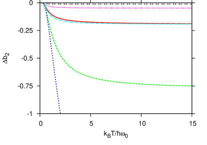
Figure 1: $\Delta b_{2}$ in 2D as a function of temperature with a model space of 160 oscillator shells and zero energy shift. The cutoff used was the function in Eq. (28). The values of $T_{0}$ and $\omega_{in}$ (in units of $\omega_{0}$) from bottom to top are $(T_{0},\omega_{in})=(0.51,5.0)$, $(0.25,5.0)$, $(0.13,5.0)$, $(0.25,2.5)$, $(0.13,5.0)$, and $(0.062,2.5)$. The $T_{0}$ values are $\omega_{in}/2\pi^{2}$ and twice and half that value.

III.1 Virial coefficients

The cut-off parameter is essential for the behavior of the expansion coefficients. The size of an appropriate value can be estimated by inspection of the effect it is designed to simulate. The first excited state appears at an excitation energy of $\hbar\omega_{r}$ which is a single quasi particle excitation. Therefore $\hbar\omega_{r}$ represents a shell gap to be overcome by thermal excitations. This gap is known to wash out at a critical temperature, $T$ given by $k_{B}T2\pi^{2}\approx\hbar\omega_{r}$, see jen73 ; boh75 . This surprisingly large factor, $2\pi^{2}\approx 19.7$, suggests a rather small relative value of $T_{0}$ proportional to $\omega_{r}$, that is $k_{B}T_{0}\approx\hbar\omega_{r}/(2\pi^{2})$.

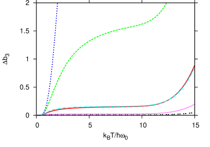
Figure 2: Same as in Fig. 1 for $\Delta b_{3}$ in 2D. The parameters are also the same but must be read from top to bottom.

To illustrate the dependence we show $\Delta b_{2}$ in Fig. 1 as function of $T$ for different interactions and cut-off values. We see the general behavior of a second order increase from zero at $T=0$, and the smooth curvature before bending over to reach the saturation value. The expansion coefficient is a rather strongly increasing function of both interaction frequency and cut-off parameter. The functional form of the cut-off function in Eq. (28) implies that the saturation value as well as saturation temperature both depend rather strongly on $T_{0}$.

The overall behavior must be understood in the model even at uninterestingly large temperatures. We continue to show $\Delta b_{3}$ in Fig. 2 for for two dimensions for the same set of parameters as in Fig. 1. Qualitatively the same behavior except for the overall opposite sign. However, the temperature dependence is faster, the saturation values are larger, as seen for the small interaction frequency with the small $T_{0}$. For higher values we observe a tendency to form a flat region which quickly becomes an increasing function.

At low temperature, the coefficients vanish since both the interacting and non-interacting partition functions go to unity at low temperature (in the abscence of any energy shift). This might seem odd since our $\Delta b_{i}$’s are the difference between a non-interacting and interacting system, which should increase at low temperatures when the interactions are more significant compared to the kinetic energy. Since both of the partition functions are small at low temperature, the only signature we see of this is that the relative differences of the partition functions, for example $(Q_{2}-Q_{2}^{(i)})/Q_{2}^{(i)}$, does increase.

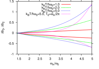
Figure 3: Virial coefficients $\Delta b_{2}<0$ and $\Delta b_{3}>0$ as a function of interaction frequency $\omega_{in}$ for three different temperatures. Notice that from Eq. (15) we always have $\omega_{in}>\sqrt{2}\omega_{0}$. On this plot, $k_{B}T_{0}/\hbar\omega_{0}=0.25$ for all curves except the short-dotted line which has $k_{B}T/\hbar\omega=5.0$ and $k_{B}T_{0}=\hbar\omega_{in}/2\pi^{2}$ (adjusted at end point on the horizontal axis).

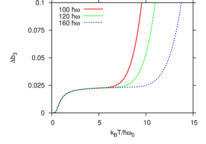
Figure 4: $\Delta b_{3}$ in 2D as a function of temperature for three different model space sizes. The cut-off function is that given in Eq. (28). The other paramters are $k_{B}T_{0}=0.25\hbar\omega_{0}$ and $\omega_{in}=2.5\omega_{0}$

The effect of the interaction frequency is plainly to increase the virial coefficient, which could be seen in Figs. 1 and 2. A more precise dependence on interaction frequency can be seen in Fig. 3. The coefficients vanish for small $\omega_{in}$, as then there is no difference between the non-interacting and interacting system, but then increase rapidly, especially after $\omega_{in}>\omega_{0}$. The increase is more dramatic at higher temperatures, which are closer to the saturation value. It does appear, however, that for any temperature the behavior of the coefficients is faster than linear.

III.2 Hilbert space and cut-off function

The apparent lack of saturation for $\Delta b_{3}$ at high temperatures is a very unsatisfactory feature. Fortunately, it seems to be an effect of the model space truncation at high excitation energies in the calculation of the partition function. This happens because of the subtle nature of the cancellation which removes the divergence and leads to saturation. The piece, $Q_{1}$, in $\Delta Q_{2}$ in Eq. (12) contains all states to infinitely high excitation energies since it is calculated analytically. This piece eventually overwhelms the $\Delta Q_{3}$ term in Eq. (12) which is calculated numerically and consequently arises from a truncated energy spectrum.

We demonstrate this in Fig. 4 where we show $\Delta b_{3}$ for three different model space sizes. The higher energies we include in the numerical calculation, the larger is the region of the flat saturation interval, and the larger temperatures before the divergence sets in. This is very reassuring allowing us to ignore the unphysical region of all temperatures above the flat region.

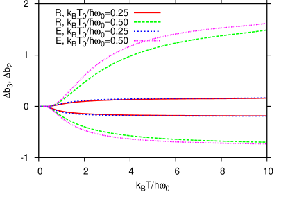
Figure 5: Virial coeffecients in 2D as a function of temperature for different cut-off functions. The rational function cutoffs, Eq. (28), are labeled with an ’R’, and the exponential cutoff, Eq. (31), with an ’E’. $\omega_{in}=2.5\omega_{0}$ was used for all of the curves.

One uncertainty in the method to recover the high-energy non-interaction limit is the function describing the disappearance of shell effects. In Fig. 5 we illustrate this dependence of the virial coefficients by results from use of different cutoff functions, that is the rational expression, Eq. (28), and the exponential functon, Eq. (31). The virial coefficients using the exponential cutoff are larger for all temperatures before finally merging into the same high temperature limit. This is due to the larger cut-off function at all temperatures which leaves the reduction to take place somehwat faster at larger temperatures although the same final saturation is reached for $T$ much larger than $T_{0}$.

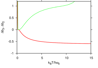
Figure 6: $\Delta b_{2}$ (lower solid line) and $\Delta b_{3}$ (upper dashed line) in 2D as a function of temperature examining the effect of the energy shift. The coeffecients behave similar to what was shown previously except at very small temperature. For this plot, $\omega_{in}=2.0\omega_{0}$ with $V_{s}=-5.81\hbar\omega_{0}$, and $k_{B}T_{0}=0.5\hbar\omega$.

III.3 Effect of the energy shift

The energy shift in the Hamiltonian has a different effect on the virial coefficient. We illustrate by the examples in Fig. 6. The large temperature limit remains finite by construction as shown explicitly in energies Eq. (29) for one case. Otherwise the behavior at large $T$ is very similar to that of zero shift, where convergence is essential or at least a flat region at high $T$ is necessary. The energies enter in the partition function in the exponent. Contributions disappear from energies much higher than the temperature.

However, at very small temperatures the same contribution from the shift can produce unphysical results. This is seen at very low $T$ in Fig. 6 where a narrow and large peak is present in both virial coefficients. The numerical reason is obvious since the negative shift divided by a small temperature produce a very large value. This occurs for temperatures much smaller than $\omega_{0}$ and much before the statistical treatment is meaningful.

The negative shift is not necessarily sufficient for a divergence at low temperatures. The shift energy must completely eliminate the zero-point energy, and thus for polarized fermions $V_{S}<-DN\hbar\omega_{r}$. The parameters in Fig. 6 provide a shift large enough in magnitude to give a spike towards large positive values at very low temperatures. This changes the sign of $\Delta b_{2}$, as the term containing the shift eventually (small $T$) becomes larger than the non-interacting term in Eq. (24).

For $\Delta b_{3}$, the singularity at zero temperature comes at a slightly higher temperature since the shift energy is three times larger than for two particles. Again this occurs for temperatures smaller than those allowing a statistical treatment.

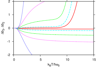
Figure 7: The virial coeffcicients in three dimensions, $\Delta b_{2}<0$ (lower lines) and $\Delta b_{3}>0$ (upper lines), as function of temperature. The cut-off temperatures, $T_{0}$, and $\omega_{in}$ is varied among the different curves. On the $\Delta b_{2}$ side (below zero) from bottom to top it is $(k_{B}T_{0}/\hbar\omega_{0},\omega_{in}/\omega_{0}=(1.00,2.5)$, $(0.50,3.5)$, $(0.50,2.5)$, $(0.50,1.5)$, and $(0.25,2.5)$. For $\Delta b_{3}$ (above zero), the lines have the parameters just listed but in the inverse ordering. For this plot, there is no energy shift $V_{S}=0$ and a model space of 160 shells is used.

III.4 Three dimensions

We have so far only shown results for two dimensions. The method is, however, as applicable in three dimensions where the coefficients look qualitatively similar to those in two dimensions, see Fig. 7. We notice the increase from zero at $T=0$, then a decreasing derivative resulting in saturation or in a tendency towards saturation, and finally the divergence at large temperature for $\Delta b_{3}$ due to mismatch between the numerical $Q_{3}$ and the analytical $Q_{1}$. The results are more sensitive to the cutoff parameter because higher powers enter in two than in three dimensions, as seen for example by comparing Eqs. (29) and (30). Indeed, if one uses $T_{0}=\omega_{in}/(2\pi^{2})$, then the magnitude of the coefficients is quite small, of order $10^{-2}$. Also, the truncation effect in $\Delta b_{3}$ is more sensitive to the cutoff parameter and can begin at comparatively low temperatures when compared to 2D, see Fig. 2.

The virial expansion is most efficient when the size of the coefficients decrease with the order. Therefore, a requirement of $\Delta b_{3}\leq\Delta b_{2}$, leads to a condition on the maximum size of $T_{0}$. This demand is more restrictive for three than for two dimensions.

IV Summary and outlook

We have discussed the virial expansion technique and a quantum mechanical formulation is sketched from an analogous classical expansion. We apply the formulated method to a harmonic approximation to the $N$-body problem for identical fermions. A key step in this approach is the adjustment of the harmonic one- and two-body parameters to pertinent properties of the corresponding two-body problem that holds information about the exact interaction which is approximated by a harmonic form. Once these are obtained, the resulting $N$-body Schrödinger equation may be solved exactly and the spectrum can be used to compute the partition function. The second and third order virial expansion coefficients are obtained by direct calculation of the two and three-body partition functions. Here we are interested in the details of the formal development of a virial expansion and we therefore vary the parameters of the harmonic interaction terms freely to study the behavior. The mapping to realistic two-body properties is straightforward.

The virial expansion can be reformulated in terms of deviations between non-interacting and interacting systems. Importantly, the virial coefficients have an unphysical divergence for large temperatures. It arises in the formulation because the increasing temperature populates higher and higher excited states. Their average properties can be very far from the ground state properties, and eventually the results should resemble those of the non-interacting system where the kinetic energy is decisive. This is achieved by modifying the energy spectrum by a function of temperature smoothly connecting the low-temperature ground state dominated and high-temperature non-interacting spectra.

To achieve the goal of removing the divergence, the modification function must reduce the initial interaction frequency to zero by a large-temperature behavior where the power of the temperature is equal to the spatial dimension of the system. The divergence is removed from the second order expansion coefficient and it turns out that the same modification function removes the divergence from the third order term. This result is highly non-trivial since the third order divergence is of a very different origin from that of second order. This is emphasized by an attempt to use an energy (in contrast to temperature) dependent modification function which removes the second order divergence but requires an additional adjustment to remove the third order divergence. The temperature modification is then the more promising approach for applications where higher orders have to be calculated.

We find that the critical temperature value describing where the adjustment of the spectrum should take place and the rate of the modification should be about $2\pi^{2}$ smaller than the two-body interaction frequency. This is an analogy to the smearing of shell effects by temperature in an $N$-body finite system described by its single-particle spectrum. This function is exponential and the rate is precisely the single-particle frequency divided by $2\pi^{2}$. In our case the modification function is chosen to have a rate of change of the $N$-body energy spectrum which is a rational function of temperature to a power that depends on dimension. However, the modification takes place on the energies appearing in the exponent of the partition function. The precise shape of the temperature modification function is not essential for the overall properties unless one consideres extreme cases. A sensible choice of modification function that regularizes the divergence will thus yield a formalism that can be adjusted to low-energy properties and make further predictions for the many-body problem.

While we have focused on two- and three-dimensional systems in the current presentation, a good testing ground for the formalism discussed would be some of the exactly solvable models that are known in one-dimensional systems sutherland04 . A good example is the $N$-boson problem with zero-range interactions studied by Lieb, Linniger, and MacGuire lieb63a for which the harmonic approximation can be applied jeremy2012 , or to dipolar molecules in one-dimensional setups where $N$-body clusterized bound states can easily form dipole1D . In the strong-coupling domain these should be well-described within a harmonic approximation approach.

In summary, we have demonstrated that the harmonic approximation employed at the Hamiltonian level gives a divergent set of virial expansion coefficients that must be regularized at high temperature. This can be done by a careful choice of temperature-dependent spectral modification that will render the virial coefficients finite at all temperatures. The ease of solving the harmonic $N$-body problem and subsequently calculating the virial coefficients makes this an attractive approach to compute many-body properties.

References

- (1) M. Thiesen, Annalen der Physik 24, 467 (1885).
- (2) H. K. Onnes, Communications from the Physical Laboratory of the University of Leiden 71, 3 (1901).
- (3) H. D. Ursell, Math. Proc. Cam. Phil. Soc. 23, 685 (1927).
- (4) T. L. Hill: Statistical Mechanics, (McGraw-Hill, New York, 1956).
- (5) E. Beth and G. E. Uhlenbeck, Physica 4, 915 (1937); B. Kahn and G. E. Uhlenbeck, Physica 5, 399 (1938).
- (6) K. Huang, Statistical Mechanics, 2nd ed. (Wiley, New York, 1987).
- (7) R. Dashen, S.-K. Ma, and H. J. Bernstein, Phys. Rev. 187, 345 (1969).
- (8) S. K. Adhikari and R. D. Amado, Phys. Rev. Lett. 27, 485 (1971).
- (9) P.-T. How and A. LeClair, Nucl. Phys. B 824, 415 (2010); J. Stat. Mech. P0302 (2010); J. Stat. Mech. P07001 (2010).
- (10) A. LeClair, E. Marcelino, A. Nicolai, and I. Roditi, Phys. Rev. A 86, 023603 (2012).
- (11) F. Brosens, J. T. Devreese, and L. F. Lemmens, Phys. Rev. E 55, 227 (1997); ibid. 55, 6795 (1997); ibid. 57, 3871 (1998); ibid. 58, 1634 (1998).
- (12) M. A. Zaluska-Kotur, M. Gajda, A. Orlowski, and J. Mostowski, Phys. Rev. A 61, 033613 (2000); J. Yan, J. Stat. Phys. 113, 623 (2003); M. Gajda, Phys. Rev. A 73, 023603 (2006);
- (13) F. Brosens, J. T. Devreese, and L. F. Lemmens, Phys. Rev. A 55, 2453 (1997); J. Tempere, F. Brosens, L. F. Lemmens, and J. T. Devreese, Phys. Rev. A 58, 3180 (1998); Phys. Rev. A 61, 043605 (2000); L. F. Lemmens, F. Brosens, and J. T. Devreese, Phys. Rev. A 59, 3112 (1999); S. Foulon, F. Brosens, J. T. Devreese, and L. F. Lemmens, Phys. Rev. E 59, 3911 (1999).
- (14) J. Tempere, F. Brosens, L. F. Lemmens, and J. T. Devreese, Phys. Rev. A 61, 043605 (2000).
- (15) J. R. Armstrong, N. T. Zinner, D. V. Fedorov, and A. S. Jensen, J. Phys. B: At. Mol. Opt. Phys. 44, 055303 (2011).
- (16) T. Busch, B. G. Englert, K. Rza̧żewski, and M. Wilkens, Found. Phys. 28, 548 (1998).
- (17) T. Stöferle, H. Moritz, K. Günter, M. Köhl, and T. Esslinger, Phys. Rev. Lett. 96, 030401 (2006); T. Volz et al., Nature Phys. 2, 692 (2006); G. Thalhammer et al., Phys. Rev. Lett. 96, 050402 (2006); C. Ospelkaus et al., Phys. Rev. Lett. 97, 120402 (2006).
- (18) W. C. Haxton and T. Luu, Phys. Rev. Lett. 89, 182503 (2002). I. Stetcu, B. R. Barrett, and U. van Kolck, Phys. Lett. B 653, 358 (2007); I. Stetcu, B. R. Barrett, U. van Kolck, and J. P. Vary, Phys. Rev. A 76, 063613 (2007); Y. Alhassid, G. F. Bertsch, and L. Fang, Phys. Rev. Lett. 100, 230401 (2008); N. T. Zinner, K. Mølmer, C. Özen, D. J. Dean, and K. Langanke, Phys. Rev. A 80, 013613 (2009); I. Stetcu, J. Rotureau, B. R. Barrett, and U. van Kolck, Ann. Phys. 325, 1644 (2010); T. Luu, M. J. Savage, A. Schwenk, and J. P. Vary, Phys. Rev. C 82, 034003 (2010); J. Rotureau, I. Stetcu, B. R. Barrett, M. C. Birse, and U. van Kolck, Phys. Rev. A 82, 032711 (2010).
- (19) J. R. Armstrong, N. T. Zinner, D. V. Fedorov, and A. S. Jensen, Europhys. Lett. 91, 16001 (2010); J. R. Armstrong, N. T. Zinner, D. V. Fedorov, and A. S. Jensen, arXiv:1112.6141; D. V. Fedorov, J. R. Armstrong, N. T. Zinner, and A. S. Jensen, Few-Body Syst. 50 395 (2011).
- (20) J. R. Armstrong, N. T. Zinner, D. V. Fedorov, and A. S. Jensen, Eur. Phys. J. D 66, 85 (2012). A. G. Volosniev, J. R. Armstrong, D. V. Fedorov, A. S. Jensen, and N. T. Zinner, arXiv:1112.2541.
- (21) N. T. Zinner, J. R. Armstrong, A. G. Volosniev, D. V. Fedorov, and A . S. Jensen, Few-Body Syst. 53, 369 (2012).
- (22) D.-W. Wang, M. D. Lukin, and E. Demler, Phys. Rev. Lett. 97, 180413 (2006).
- (23) A. Pikovski, M. Klawunn, G. V. Shlyapnikov, and L. Santos, Phys. Rev. Lett. 105, 215302 (2010); N. T. Zinner, B. Wunsch, D. Pekker, and D.-W. Wang, Phys. Rev. A 85, 013603 (2012).
- (24) S.-M. Shih and D.-W. Wang, Phys. Rev. A 79, 065603 (2009).
- (25) M. Klawunn, A. Pikovski, and L. Santos, Phys. Rev. A 82, 044701 (2010).
- (26) M. A. Baranov, A. Micheli, S. Ronen, and P. Zoller, Phys. Rev. A 83, 043602 (2011).
- (27) A. G. Volosniev, D. V. Fedorov, A. S. Jensen, and N. T. Zinner, Phys. Rev. Lett. 106, 250401 (2011); Phys. Rev. A 85, 023609 (2012); A. G. Volosniev, N. T. Zinner, D. V. Fedorov, A. S. Jensen, and B. Wunsch, J. Phys. B: At. Mol. Opt. Phys. 44, 125301 (2011).
- (28) J. R. Armstrong, N. T. Zinner, D. V. Fedorov, and A. S. Jensen, Phys. Rev. E 85, 021117 (2012).
- (29) L. F. Lemmens, F. Brosens, and J. T. Devreese, Solid State Comm. 109, 615 (1999).
- (30) S. N. Klimin, V. M. Fomin, F. Brosens, and J. T. Devreese, Phys. Rev. B 69, 235324 (2004).
- (31) F. Brosens, S. N. Klimin, and J. T. Devreese, Phys. Rev. B 71, 214301 (2005).
- (32) M. Horikoshi, S. Nakajima, M. Ueda, and T. Makaiyama, Science 327, 442 (2010); S. Nascimbéne et al., Nature 463, 1057 (2010); N. Navon, S. Nascimbéne, F. Chevy, and C. Salomon, Science 328, 729 (2010); C. Cao et al., Science 331, 58 (2011); M. J. H. Ku, A. T. Sommer, L. W. Clark, and M. W. Zwierlein, Science 335, 563 (2012).
- (33) T.-L. Ho and E. J. Mueller, Phys. Rev. Lett. 92, 160404 (2004); H. Hu , P. D. Drummond, and X.-J. Liu, Nature Phys. 3, 469 (2007); X.-J. Liu, H. Hu, and P. D. Drummond, Phys. Rev. Lett. 102, 160401 (2009); X.-J. Liu, H. Hu, and P. D. Drummond, Phys. Rev. A 82, 023619 (2010); S.-G. Peng, S.-Q. Li, P. D. Drummond, and X.-J. Liu, Phys. Rev. A 83, 063618 (2011); X. Leyronas, Phys. Rev. A 84, 053633 (2011); D. B. Kaplan and S. Sun, Phys. Rev. Lett. 107, 030601 (2011).
- (34) J. E. Mayer and M. G. Mayer: Statistical Mechanics, (Wiley, New York, 1940).
- (35) L. E. Reichl: A modern course in statistical physics, (J. Wiley and Sons, New York, 2nd ed., 1998).
- (36) H. Hu, X.-J. Liu, and P. D. Drummond, New J. Phys. 12, 063038 (2010).
- (37) Z. Idziaszek and T. Calarco, Phys. Rev. Lett. 96, 013201 (2006); Z. Idziaszek, Phys. Rev. A 79, 062701 (2009).
- (38) K. Kanjilal and D. Blume, Phys. Rev. A 73, 060701(R) (2006); N. T. Zinner, J. Phys. A: Math. Theor. 45, 205302 (2012).
- (39) P. K. Sørensen, D. V. Fedorov, A. S. Jensen, and N. T. Zinner, Phys. Rev. A 86, 052516 (2012).
- (40) R. V. E. Lovelace and T. J. Tommila, Phys. Rev. A 35, 3597 (1987); G. Baym and C. J. Pethick, Phys. Rev. Lett. 76, 6 (1996).
- (41) H. Fu, Y. Wang, and B. Gao, Phys. Rev. A 67, 053612 (2003); N. T. Zinner and M. Thøgersen, Phys. Rev. A 80, 023607 (2009); N. T. Zinner, arXiv:0909.1314; M. Thøgersen, N. T. Zinner, and A. S. Jensen, Phys. Rev. A 80, 043625 (2009).
- (42) J. R. Armstrong, N. T. Zinner, D. V. Fedorov, and A. S. Jensen, Physica Scripta T151, 014061 (2012).
- (43) X.-J. Liu, H. Hu, and P. D. Drummond. Phys. Rev. B 82, 054524 (2010).
- (44) A. S. Jensen and J. Damgaard, Nucl.Phys. A 203, 578 (1973).
- (45) A. Bohr and B. R. Mottelson: Nuclear Structure, Vol 1, (Benjamin, New York, 1969).
- (46) B. Sutherland: Beautiful Models, (World Scientific Publishing Co., Singapore, 2004); R. J. Baxter: Exactly Solved Models in Statistical Mechanics, (Academic Press, New York, 1982); V. E. Korepin: Exactly Solvable Models of Strongly Correlated Electrons, (World Scientific Publishing Co., Singapore, 1994).
- (47) E. Lieb and W. Liniger, Phys. Rev. 130, 1605 (1963); E. Lieb, Phys. Rev. 130, 1616 (1963); J. MacGuire, J. Math. Phys. 5, 622 (1964).
- (48) B. Wunsch et al., Phys. Rev. Lett. 107, 073201 (2011); M. Dalmonte, P. Zoller, and G. Pupillo, Phys. Rev. Lett. 107, 163202 (2011); N. T. Zinner et al., Phys. Rev. A 84, 063606 (2011); M. Knap, E. Berg, M. Ganahl, and E. Demler, Phys. Rev. B 86, 064501 (2012); M. Bauer and M. M. Parish, Phys. Rev. Lett. 108, 255302 (2012).