Low–dimensional $q$–tori in FPU lattices:
dynamics and localization properties

Abstract

Recent studies on the Fermi-Pasta-Ulam (FPU) paradox, like the theory of $q$–breathers and the metastability scenario, dealing mostly with the energy localization properties in the FPU space of normal modes ($q$–space), motivated our first work on $q$–tori in the FPU problem [8]. The $q$–tori are low-dimensional invariant tori hosting trajectories that present features relevant to the interpretation of FPU recurrences as well as the energy localization in $q$–space. The present paper is a continuation of our work in [8]. Our new results are: We extend a method of analytical computation of $q$–tori, using Poincaré–Lindstedt series, from the $\beta$ to the $\alpha$–FPU and we reach significantly higher expansion orders using an improved computer–algebraic program. We probe numerically the convergence properties as well as the level of precision of our computed series. We develop an additional algorithm in order to systematically locate values of the incommensurable frequencies used as an input in the PL series construction of $q$–tori corresponding to progressively higher values of the energy. We generalize a proposition proved in [8] regarding the so-called ‘sequence of propagation’ of an initial excitation in the PL series. We show by concrete examples how the latter interprets the localization patterns found in numerical simulations. We focus, in particular, on various types of extensive initial excitations that lead to $q$–tori solutions with exponentially localized profiles. Finally, we discuss the relation between $q$–tori, $q$–breathers (viewed as one-dimensional $q$–tori), and the so–called ‘FPU–trajectories’ invoked in the original study of the FPU problem.

1 Introduction

In the well known numerical experiment of Fermi, Pasta and Ulam in 1955, reported in [10], a dynamical system consisting of $N$ nonlinearly coupled oscillators showed an integrable–like behavior, contradicting the ergodic hypothesis of Fermi. This surprising result motivated numerable historical works, from Korteweg - de Vries, solitons and Toda to ergodic theory etc., that together with the KAM theorem discovered in the same period, changed the perspective of statistical mechanics, ergodic and perturbation theory.

The FPU recurrences in the energies of normal modes, observed in [10] when exciting one or few low–frequency normal modes, lead to the conclusion that energy transfer between modes is practically frozen, with only few modes sharing the total energy, leaving the system far from equilibrium (see also the review [23]). A careful inspection of the averaged in time energy spectra shows an exponentially localized profile in $q$–space, characterized by a ‘plateau’ in the low–frequency part of the energy spectrum, a so–called natural packet of modes [3, 4, 18], accompanied by an exponential tail of the energy distribution for the remaining modes. This state of the system is called ‘metastable state’ [1, 16, 24, 28, 29] and recent studies on its persistence and times to equipartition are given in [2].

On the other hand, it was observed that there exist periodic orbits called $q$–breathers, introduced in the series of works [11]–[15], [21], [22], which share many common features with trajectories rising by the excitation of just one normal mode (called ‘FPU–trajectories’). These Lyapunov orbits are continuations of the linear modes, which, at low energies, have a similar exponentially localized energy spectrum as the FPU–trajectories, characterized by an exponent that depends logarithmically on the system’s parameters.

This latter remark initiated the idea of studying trajectories corresponding to the excitation of more than one linear modes, i.e. lying on tori of low dimensionality in the FPU phase space. These tori were named $q$–tori in [8], and numerical evidence of their existence came out from the implementation of the method of Poincaré – Lindstedt (PL) series. We should stress at this point that, while the existence of $q$–breathers is guaranteed by basic theorems on the continuation of periodic orbits, the corresponding demonstration for $q$–tori would require proving the convergence of the associated PL series. A rigorous proof appears at present hardly tractable. However, in the present paper we will provide numerical tests showing that our computed series exhibit the behavior of convergent PL series. In particular, we identify near-cancellations between terms of a big absolute size, leaving a small residual in the final series. Let us note that precisely this mechanism has been invoked in well known formal proofs of the convergence of Lindstedt series in simple models [9, 17]. Furthermore, as in [8] we employ the GALI indicator [32], thus obtaining further evidence that our computed solutions lie on low-dimensional tori. Finally, we demonstrate that the $q$- tori exhibit a number of features not encountered in $q$–breathers. However, we emphasize that $q$–tori and $q$–breathers should not be regarded as competitive theories, but rather as complementary interpretation tools for the FPU localization phenomena.

We finally note that the study of FPU trajectories presenting energy localization by various means of classical perturbation theory is a known subject (for an early implementation of the simple Birkhoff normal form approach see [25]; see also references in [18]). In particular, the problem of motions on or close to low-dimensional manifolds using the classical method of Birkhoff was studied in [19]. As commented in [8], this approach leads to Nekhoroshev-like estimates for the time of stability of motions. However, the corresponding estimates have a bad behavior as $N\rightarrow\infty$. For an alternative approach to the same problem using a ‘resonant’ Birkhoff construction see [18]. On the other hand, the fact that we find indications about cancellations in our PL series implies that the $q$–tori constructed by the present method should be recoverable also by some ‘indirect’ (i.e. Kolmogorov-like normal form) approach. However, one can easily check that a recently proposed algorithm for the computation of low-dimensional tori via normal forms [31] has different divisors than in our construction. Thus, we leave the question of the existence of an appropriate Kolmogorov algorithm for the FPU $q$–tori as an open problem.

The main results and the content of this paper are stated as follows: After introducing the FPU model in Section 2, we sketch the construction of $q$–tori by Poincaré–Lindstedt series in Section 3. We also present our numerical indications regarding the convergence of the PL series with the help of a concrete example referring to a two-dimensional $q$–torus solution.

In Section 4, we give an example of a 4-dimensional $q$–torus solution. Here, we focus on the energy localization properties of such a torus. Furthermore, we compare this object with a corresponding so-called ‘FPU–trajectory’ (subsection 4.1), finding results analogous to the study in [29], but for groups of modes rather than one mode.

Section 5 deals with an extension of our proposition found in [8], where, we prove the so–called propagation of initial excitations of modes for both the $\alpha$ and $\beta$ FPU models. In the context of perturbation theory, an initial excitation means a particular selection of a subset of modes in $q$–space for which we consider an oscillation with non–zero amplitude at the zero order of perturbation theory. Then, this excitation propagates to new modes at subsequent orders, giving justification to the observed exponential localization profile of $q$–tori.

In section 6 we give several numerical examples and localization profiles associated to $q$–tori, and we compare them with the predictions of the proposition developed in section 5. We examine, in particular:

i) low–frequency packet excitations (subsection 6.1), paying emphasis on so-called extensive initial excitations, i.e. ones in which the number of initially excited consecutive modes varies proportionally to $N$. We predict, based on a leading term analysis of the associated PL series, that the form of their energy spectrum has an exponentially localized profile with a slope that depends logarithmically on the specific energy $\varepsilon=E/N$ and on the system’s parameters.

ii) ‘arbitrary’ initial excitations (subsection 6.2), i.e. excitations of modes chosen arbitrarily within the whole spectrum, leading to the formation of a variety of localization patterns, whose form is predicted theoretically and confirmed by numerical experiments.

iii) ‘generalized packet excitations’ (subsection 6.3), i.e. excitations of extensive packets of modes in various arbitrarily chosen parts of the spectrum. In this case we study the formation of local exponential profiles far from the low-frequency part of the spectrum.

iv) $q$–breathers, examined as a particular case of one-dimensional $q$–tori (subsection 6.4). In this case we examine how the $q$–breathers compare with the FPU–trajectories studied in the original FPU report, i.e. for the lowest frequency mode excitation, but also for a high frequency mode excitation. In particular, we point out the similarity between $q$–breathers and FPU trajectories regarding their energy localization pattern, but also their different behavior related to the phenomenon of FPU recurrences at higher energies.

Section 7 is a summary of our basic conclusions from the present study and a discussion on future perspectives.

2 The Fermi Pasta Ulam model

The FPU Hamiltonian for a lattice of $N-1$ particles reads:

$$H={1\over 2}\sum_{k=1}^{N-1}y_{k}^{2}+{1\over 2}\sum_{k=0}^{N-1}(x_{k+1}-x_{k})^{2}+{\alpha\over 3}\sum_{k=0}^{N-1}(x_{k+1}-x_{k})^{3}+{\beta\over 4}\sum_{k=0}^{N-1}(x_{k+1}-x_{k})^{4}$$ (1)

where $x_{k}$ is the $k$–th particle’s position with respect to equilibrium and $y_{k}$ its canonically conjugate momentum. Fixed boundary conditions are defined by setting $x_{0}=x_{N}=0$. The cases $\alpha\neq 0$, $\beta=0$, and $\alpha=0$, $\beta\neq 0$ are called FPU–$\alpha$ and FPU–$\beta$ model respectively.

The normal mode canonical variables $(Q_{q},P_{q})$ are introduced by the linear canonical transformation

$$x_{k} = \sqrt{2\over N}\sum_{q=1}^{N-1}Q_{q}\sin\left({qk\pi\over N}\right)$$

$$y_{k} = \sqrt{2\over N}\sum_{q=1}^{N-1}P_{q}\sin\left({qk\pi\over N}\right).$$ (2)

Substitution of (2) into (1) yields the Hamiltonian in the normal mode space ($q$–space):

$$H={1\over 2}\sum_{q=1}^{N-1}{(P_{q}^{2}+\Omega_{q}^{2}Q_{q}^{2})}+{\alpha\over 3\sqrt{2N}}\sum_{q,l,m=1}^{N-1}B_{qlm}\Omega_{q}\Omega_{l}\Omega_{m}Q_{q}Q_{l}Q_{m}$$ (3)

$$+{\beta\over 8N}\sum_{q,l,m,n=1}^{N-1}C_{qlmn}\Omega_{q}\Omega_{l}\Omega_{m}\Omega_{n}Q_{q}Q_{l}Q_{m}Q_{n}$$

with normal mode frequencies

$$\Omega_{q}=2\sin\left({q\pi\over 2N}\right),~{}~{}~{}1\leq q\leq N-1~{}~{}~{}.$$ (4)

The harmonic energy $E_{q}$ of each normal mode $q$ is given by

$$E_{q}={1\over 2}(P_{q}^{2}+\Omega_{q}^{2}Q_{q}^{2})~{}~{}~{}.$$ (5)

The coefficients $B_{qlm}$ and $C_{qlmn}$ are non–zero only for particular combinations of the indices $q,l,m,n$, namely

$$B_{qlm} = \sum_{\pm}(\delta_{q\pm l\pm m,0}-\delta_{q\pm l\pm m,2N})$$

$$C_{qlmn} = \sum_{\pm}(\delta_{q\pm l\pm m\pm n,0}-\delta_{q\pm l\pm m\pm n,2N})~{}~{}.$$ (6)

In the above expressions, all possible combinations of the $\pm$ signs must be taken into account. In the new canonical variables, the equations of motion are:

$$\ddot{Q}_{q}+\Omega_{q}^{2}Q_{q}=-{\alpha\over{\sqrt{2N}}}\sum_{l,m=1}^{N-1}B_{qlm}\Omega_{q}\Omega_{l}\Omega_{m}Q_{l}Q_{m}$$

$$-{\beta\over 2N}\sum_{l,m,n=1}^{N-1}C_{qlmn}\Omega_{q}\Omega_{l}\Omega_{m}\Omega_{n}Q_{l}Q_{m}Q_{n}~{}~{}.$$ (7)

3 Construction of $q$–tori by Poincaré–Lindstedt series

3.1 PL Algorithm

As in [8], we will now construct quasi-periodic solutions lying on $q$–tori by implementing the method of Poincaré–Lindstedt series. The main steps of our constructive algorithm are the following:

As a starting point we consider first the trivial case $\alpha=\beta=0$. Let

$${\cal D}_{0}\equiv\{q_{1},q_{2},\ldots,q_{s}\},~{}~{}\mbox{where}~{}~{}1\leq q_{i}\leq N-1~{}~{}\mbox{with}~{}~{}q_{i}<q_{j},~{}~{}\mbox{for}~{}~{}i<j$$

be an arbitrary set of $s<N$ modes, called hereafter ‘seed modes’ (in analogy to [11], where the case $s=1$ corresponding to $q$–breathers is considered). The set of functions $Q_{q_{i}}(t)=A_{q_{i}}\cos(\Omega_{q_{i}}t+\phi_{q_{i}})$, $i=1,\ldots,s$ and $Q_{q}(t)=0$ if $q\notin{\cal D}_{0}$, constitutes a particular solution of the linear system. The resulting trajectory lies on a $s$–dimensional torus, provided that the frequencies $\Omega_{q_{i}}$ of Eq. (4) satisfy no commensurability relation. This turns out to be always the case if $N-1$ is a prime number or $\log_{2}N\in\mathbf{N}^{*}$ [20]. If, on the other hand, the frequencies $\Omega_{q_{i}}$ satisfy $s^{\prime}$ linearly independent commensurability relations ($0<s^{\prime}<s$), the trajectories lie on a ‘resonant torus’ of dimension $s-s^{\prime}$, which is a sub–manifold of the original $q$–torus of dimension $s$.

Passing now to the nontrivial case $a\neq 0$, or $\beta\neq 0$, we aim to define quasi–periodic trajectories lying on $s$–dimensional tori. To this end, let $\omega_{q_{i}}$, $i=1,\ldots,s$ be a set of frequencies with fixed values chosen in advance, which are incommensurable between themselves as well as with each one of the linear frequencies $\Omega_{q}$ of the remaining modes $q\notin{\cal D}_{0}$. We then determine formal solutions $Q_{q}(t)$, $q=1,\ldots,N-1$ containing only trigonometric terms of the form $\cos(n\cdot(\omega t+\phi))$, where $n\equiv(n_{1},n_{2},\ldots,n_{s})$ is an $s$–dimensional integer vector and $\omega\equiv(\omega_{q_{1}},\ldots,\omega_{q_{s}})$, $\phi\equiv(\phi_{q_{1}},\ldots,\phi_{q_{s}})$ are the frequency and phase vectors respectively.

According to the PL method, these solutions are written as series in powers of a small parameter $\mu=\alpha/\sqrt{2N}$, or $\mu=\beta/2N$, namely:

$$Q_{q}(t)=\sum_{k=0}^{\infty}\mu^{k}Q_{q}^{(k)}(t),~{}~{}~{}q=1,\ldots,N-1~{}~{}.$$ (8)

The series terms $Q_{q}^{(k)}$ are computed step by step. The zero order terms are set as

$$Q_{q}^{(0)}(t)=\left\{\begin{array}[]{rl}A_{q}\cos(\omega_{q}t+\phi_{q}),&\mbox{if}~{}q\in{\cal D}_{0}\\ 0,&\mbox{otherwise}~{}~{}.\end{array}\right.$$ (9)

We emphasize that the amplitudes $A_{q_{i}}$, $i=1,\ldots,s$ are unknown quantities to be specified at the end of the process. In the computer–algebraic program, $A_{q_{i}}$ are symbols carried all along the construction of the PL series, while the frequencies $\omega_{q_{i}}$ are substituted at the beginning by their selected numerical values. However, according to the PL method, the frequencies $\omega_{q_{i}}$ must also be expressed in the form of a series in powers of the amplitudes $A_{q_{i}}$, namely

$$\omega_{q_{i}}=\Omega_{q_{i}}+\sum_{k=1}^{\infty}\mu^{k}\omega_{q_{i}}^{(k)}(A_{q_{1}},\ldots,A_{q_{s}})~{}~{}.$$ (10)

The functions $\omega_{q_{i}}^{(k)}(A_{q_{1}},\ldots,A_{q_{s}})$ are polynomials of the amplitudes $A_{q_{1}},\ldots,A_{q_{s}}$, of order $k+1$ in the $\alpha$–case, or $2k+1$ in the $\beta$–case.

Substituting Eqs.(8) and (10) in the equations of motion (2), we find the following equations to be solved at order $k$: for the FPU–$\alpha$ model we have

$$\ddot{Q}_{q}^{(k)}+\omega_{q}^{2}Q_{q}^{(k)} = \sum_{n_{1}=1}^{k}\sum_{n_{2}=0}^{n_{1}}\omega_{q}^{(n_{2})}\omega_{q}^{(n_{1}-n_{2})}Q_{q}^{(k-n_{1})}$$

$$- \Omega_{q}\sum_{l,m=1}^{N-1}\Omega_{l}\Omega_{m}B_{qlm}\sum_{\mathop{n_{1,2}=0}\limits_{n_{1}+n_{2}=k-1}}^{k-1}Q_{l}^{(n_{1})}Q_{m}^{(n_{2})},~{}~{}~{}\mbox{if $q\in{\cal D}_{0}$}$$

$$\ddot{Q}_{q}^{(k)}+\Omega_{q}^{2}Q_{q}^{(k)} = -\Omega_{q}\sum_{l,m=1}^{N-1}\Omega_{l}\Omega_{m}B_{qlm}\sum_{\mathop{n_{1,2}=0}\limits_{n_{1}+n_{2}=k-1}}^{k-1}Q_{l}^{(n_{1})}Q_{m}^{(n_{2})},~{}~{}~{}\mbox{if $q\notin{\cal D}_{0}$}$$

while for the FPU–$\beta$ model we have

$$\ddot{Q}_{q}^{(k)}+\omega_{q}^{2}Q_{q}^{(k)} = \sum_{n_{1}=1}^{k}\sum_{n_{2}=0}^{n_{1}}\omega_{q}^{(n_{2})}\omega_{q}^{(n_{1}-n_{2})}Q_{q}^{(k-n_{1})}$$

$$- \Omega_{q}\sum_{l,m,n=1}^{N-1}\Omega_{l}\Omega_{m}\Omega_{n}C_{qlmn}\sum_{\mathop{n_{1,2,3}=0}\limits_{n_{1}+n_{2}+n_{3}=k-1}}^{k-1}Q_{l}^{(n_{1})}Q_{m}^{(n_{2})}Q_{n}^{(n_{3})},~{}~{}~{}\mbox{if $q\in{\cal D}_{0}$}$$

$$\ddot{Q}_{q}^{(k)}+\Omega_{q}^{2}Q_{q}^{(k)} = -\Omega_{q}\sum_{l,m,n=1}^{N-1}\Omega_{l}\Omega_{m}\Omega_{n}C_{qlmn}\sum_{\mathop{n_{1,2,3}=0}\limits_{n_{1}+n_{2}+n_{3}=k-1}}^{k-1}Q_{l}^{(n_{1})}Q_{m}^{(n_{2})}Q_{n}^{(n_{3})},~{}~{}~{}\mbox{if $q\notin{\cal D}_{0}$.}$$

By integrating either Eqs.(3.1) or (3.1), secular terms of the form $t\sin(\omega_{q}t)$ appear in the right hand side (when $q\in{\cal D}_{0}$), at even orders in the FPU–$\alpha$ and at all orders in the FPU–$\beta$. The requirement to eliminate all secular terms leads to an algebraic expression for the frequency correction terms $\omega_{q_{i}}^{(k)}$, $i=1,\ldots,s$. After eliminating the secular terms, direct integration of Eqs.(3.1) or (3.1) yields the solution of the series terms $Q_{q}^{(k)}(t)$.

Each term in both series (8) and (10) depends, now, on the yet unspecified amplitudes $A_{q_{i}}$. However, since the numerical values of the frequencies $\omega_{q_{i}}$ are specified in advance, the series (10) can be solved for the amplitudes $A_{q_{i}}$. In practice, we solve the set of equations resulting from finite truncations of the series (10). Thus, the amplitudes $A_{q_{i}}$ are also specified with finite accuracy. After determining the values of the $A_{q_{i}}$, substitution into the series (8) yields also numerical coefficients for all series terms $Q_{q}^{(k)}(t)$. Thus, we specify approximately a $q$–torus solution given by finite truncations of the functions $Q_{q}(t)$ for all $q=1,\ldots,N-1$.

3.2 Convergence and precision tests – Torus dimension

The existence of a solution of Eqs.(10) for a fixed choice of frequency values $\omega_{q_{i}}$, along with the convergence of the series (8) for that particular solution, constitutes a proof that a $q$–torus with the so chosen frequencies exists.

In practice, we can hardly provide such a proof by rigorous means. Instead, as mentioned already we work with finite truncations of the PL series. In [8] we computed only low order truncations, i.e. for orders not higher than three. In order to probe the behavior of our series we developed a computer–algebraic program able to perform high order computations of the PL series. In the limiting case of one-dimensional $q$–tori, i.e., $q$–breathers, we were able to reach expansion orders as high as 200. However, more interesting is the case of two– (or more) dimensional tori, where quite small divisors are present. Despite this fact, it is known from theoretical works [9], [17] that the PL series exhibit near-cancellations between terms of large size generated in the series by the recursive appearance of small divisors. Such near-cancellations have been shown to lead to the convergence of the PL series for diophantine frequencies in simple Hamiltonian models.

In our particular model, we observe numerically the appearance of near-cancellations in our computed PL series. One example is shown in Fig.1, referring to $N=16$, $a=0.33$, where, at the zeroth order of the PL series, we ‘excite’, i.e. consider a non-zero amplitude at the zeroth order for the modes $q_{1}=1$ and $q_{2}=2$. We construct a series representing a 2D $q$–torus with frequencies $\omega_{1}=0.19626$, $\omega_{2}=0.39046$. These frequencies are commensurable beyond the fifth decimal digit, but they can be considered as practically incommensurable regarding the divisors they generate up to our maximum reached expansion order $k=30$.

The resulting solution corresponds to a total energy $E=0.02345$. Computing the average harmonic energy for each mode (up to a time $T$), given by $\overline{E}_{q}=(1/T)\int_{0}^{T}(P_{q}(t)^{2}+\Omega_{q}^{2}Q_{q}(t)^{2})dt$, where $Q_{q}(t)$, $P_{q}(t)=\dot{Q}_{q}(t)$ are the theoretical functions determined by the truncated PL series, we arrive at the profile shown in Fig.1(a). This profile exhibits exponential localization, since the energy of the $q$–th mode decays exponentially with $q$. This phenomenon will be studied with more detailed examples in sections 4 to 6 below.

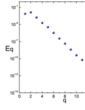
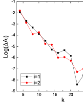
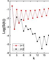
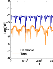
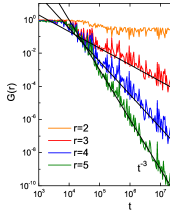
Figure 1: (a) The exponentially localized energy spectrum of a 2–torus. (b) The logarithm of the absolute errors $\Delta A_{i}(k)=|A_{i}(k+2)-A_{i}(k)|$ for $i=1,2$ versus the order $k$. (c) The logarithm of the sums $S_{1}$ and $S_{2}$ defined in Eq.(14) and Eq.(15) respectively versus $k$. (d) The relative errors in time of the harmonic and the total energy calculated by the PL method. (e) The GALI indices for $r=2,\ldots,5$.

In order, now, to probe the behavior of our series with increasing truncation order, we perform a number of numerical tests leading to Figs.1(b),(c),(d), and (e).

Figure 1(b) shows, on a logarithmic scale, the absolute errors in the determination of the amplitudes $A_{1}$,$A_{2}$ using numerical solutions of finite truncations of Eqs.(10) at various (increasing) orders. The plotted quantities are $\Delta A_{1}(k)=|A_{1}(k+2)-A_{1}(k)|$ and $\Delta A_{2}(k)=|A_{2}(k+2)-A_{2}(k)|$, where $A_{1}(k),A_{2}(k)$ and $A_{1}(k+2),A_{2}(k+2)$ are approximations to the amplitudes as determined by solving numerically Eqs.(10) truncated at the $k-th$ and $k+2$nd orders respectively. We note that the error in the determination of the amplitudes decreases as the truncation order increases, up to the order $k=24$, while afterwards the error slightly increases. The increase appears after the error reaches a minimum level $\Delta A\sim 10^{-8}$–$10^{-7}$, while the frequencies themselves become commensurable at this level of precision. Thus, in subsequent calculations we use the values of the amplitudes found at the order $k=24$, up to which the behavior of the series appears as convergent. The computed values of the amplitudes are $A_{1}=0.5848897$, $A_{2}=0.4115552$.

Figure 1(c) shows now the main effect regarding the appearance of near-cancellations in our series. After completing the calculations up to the $k$–th order, we re-cast all computed series terms $Q_{q}^{(k)}(t)$ under the form:

$$Q_{q}^{(k)}(t)=\sum_{m_{1},m_{2}}\left(\sum_{i,j}h^{(k)}_{m_{1},m_{2},i,j}A_{1}^{i}A_{2}^{j}\right)\cos[m_{1}(\omega_{1}t+\phi_{1})+m_{2}(\omega_{2}t+\phi_{2})]~{}~{},$$ (13)

where the sums are over integers $m_{1},m_{2},i,j$ whose range depends on $k$. Then, focusing for example on $q=1$, the upper curve in Fig.1(c) shows the value of the sum:

$$S_{1}(k)=\sum_{m_{1},m_{2}}\sum_{i,j}|h^{(k)}_{m_{1},m_{2},i,j}A_{1}^{i}A_{2}^{j}|$$ (14)

while the lower curve shows the value of the sum:

$$S_{2}(k)=\sum_{m_{1},m_{2}}\Bigg{|}\left(\sum_{i,j}h^{(k)}_{m_{1},m_{2},i,j}A_{1}^{i}A_{2}^{j}\right)\Bigg{|}~{}~{}.$$ (15)

In words, the upper sum represents the absolute sum of all individual Fourier coefficients appearing in the series at the order $k$, while, in the lower sum, all coefficients corresponding to the same harmonics $\cos[m_{1}(\omega_{1}t+\phi_{1})+m_{2}(\omega_{2}t+\phi_{2})]$ are grouped first together and summed algebraically (as actually happens in the real series after substitution of the numerical values of the amplitudes). We now observe that the latter summation leads to a near–cancellation of terms of increasing size, leaving a residual which decreases as $k$ increases. As a result, the cancellation takes place up to four orders of magnitude compared to the size of each independent term of the PL series at the order $k=14$. The overall size of the terms of $Q_{1}^{(k)}$ at $k=14$ is about $10^{-5}$. However, as shown in Fig.1(c), beyond the order 14 numerically we cannot observe a cancellation better than one part in $10^{4}$. We attribute this fact to the finite precision by which the amplitudes $A_{1}$, $A_{2}$ have been specified. Nevertheless, despite a slight increase after $k=14$, the upper and lower curves in Fig.1(c) appear to move one parallel to the other on a logarithmic scale, indicating that the cancellations take place at all computed orders beyond $k=14$.

As an independent test of the precision of our series computations, Fig.1(d) shows the time evolution of the relative harmonic and total energy, $RE=(E(t)-E(0))/E(0)$, found by substituting the functions $Q_{q}(t)$, $P_{q}(t)$, as computed by our truncated PL series, into the harmonic part or the total Hamiltonian (3). For an exact solution, the harmonic energy undergoes some time variations due to the presence of the cubic terms in the Hamiltonian, whose size in our case is of order $\sim 10^{-2}$. On the other hand, the value of the full Hamiltonian energy should be a preserved quantity. Using our truncated series, we observe some fluctuations in the total energy which indicate an error of the level of $10^{-4}$. On the other hand, the total harmonic energy undergoes fluctuations at the expected level $10^{-2}$.

As a final test, we implement (as in [8]) the method of the Generalized Alignment Index (GALI) [32], which determines the dimension of a stable low-dimensional torus by the temporal behavior of a set of indices (denoted G₂, G₃, …) computed via an integration of the variational equations of motion along with the original ones. We recall that each index $G_{r}$ represents the $r$–volume of $r$ unitary deviation vectors. In the case of chaotic orbits, all indices $G_{r}$ decay exponentially in time. However, in the case of regular quasi-periodic orbits, the indices $G_{r}$ obtain an asymptotically constant value in time for $r$ smaller or equal to the dimension of the torus on which the orbit lies, while they decay by power laws for $r$ larger than the torus dimension (see [7, 32, 33] for more details).

Figure 1(e) shows the behavior of the indices $G_{r}$ for $r=2,3,4,5$, for an orbit integrated numerically with initial conditions as specified by our truncated series solution at the time $t=0$. We observe that even after a quite long integration time ($10^{9}$), the index $G_{2}$ appears so be stabilized to a nearly constant value, while all other indices decay in time by the power laws $t^{-1}$, $t^{-2}$, and $t^{-3}$ respectively. This behavior implies that our initial conditions lie indeed on a 2D-torus embedded in the 30–dimensional phase space of the considered FPU system.

4 A further example. Comparison of $q$–torus and ‘FPU trajectory’

In order to construct the two-dimensional $q$–torus PL series solution of the previous section, a specific choice of values for the frequencies $\omega_{1}$ and $\omega_{2}$ was made. In general, such choices lead to formal series of the form (10) for which there is no a priori guarantee that i) real-valued solutions for the amplitudes $A_{q_{i}}$ exist, and ii) if they exist, that they lead to convergent series (8). In order to circumvent this difficulty, we have developed a step-by-step algorithm by which we specify appropriate sets of numerical values $\omega_{q_{i}}$ for constructing $q$–torus solutions. For fixed $N$ and choice of $q_{i}$, this algorithm allows to move in frequency space, by specifying sets of values $\omega_{q_{i}}$ of progressively higher difference from the unperturbed frequencies $\Omega_{q_{i}}$. Using the so-determined values of the frequencies $\omega_{q_{i}}$ we nearly always find real-valued solutions $A_{q_{i}}$ of the equations (10) (in truncated form). This, in turn, allows to determine series of the form (8) exhibiting an apparently convergent behavior according to all numerical criteria set in section 3. In this way we construct approximate $q$–torus solutions corresponding to progressively higher values of the energy.

The above step-by-step algorithm for the determination of frequency values is discussed in 7. Implementing this algorithm in the FPU–$\alpha$ model with $N=32$, and an initial excitation of the 4 lowest frequency modes $q_{1}=1$, $q_{2}=2$, $q_{3}=3$, $q_{4}=4$, we determine sets of values $\omega_{1}$, $\omega_{2}$, $\omega_{3}$, $\omega_{4}$ yielding $q$–torus solutions corresponding to progressively higher energy. For each set we solve numerically the truncated Eqs.(10) in order to specify the corresponding values of the amplitudes $A_{1}$, $A_{2}$, $A_{3}$, $A_{4}$.

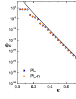
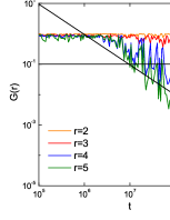
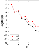
Figure 2: (a) Normalized averaged exponential spectra $e_{\kappa}$ versus $\kappa=q/N$ for the system with ${\cal D}_{0}=\{1,2,3,4\}$, $\alpha=0.33$, $E=0.000182466$, $N=32$, for a total time $T=10^{6}$. The blue spheres correspond to a $q$–torus construction with the truncated PL series, denoted $Q_{q}^{PL,11}(t)$. The orange triangles correspond to a numerical solution, denoted $Q_{q}^{PLn,11}(t)$, obtained by numerically integrating the FPU equations of motion with initial conditions $Q_{q}^{PL,11}(0)$, $P_{q}^{PL,11}(0)$. The continuous line is $\log(E_{q}/E)=3.49545-36.6613\kappa-2\log(\kappa)$. (b) GALI indices (see text) for $r=2,3,4,5$ calculated for the orbit of the orange spectrum in (a). (c) The logarithm of the sums $S_{1}$ and $S_{2}$ defined in Eq.(14) and Eq.(15) respectively versus $k$.

Figure 2 refers to a $q$–torus solution of this form computed for the numerical values for the frequencies and amplitudes given in the first group of the table in 7. The corresponding series (8) are truncated at the order $k_{0}=11$. We refer to such analytical (i.e. truncated series) solutions by the notation $Q_{q}^{PL,k_{0}}(t)$. However, in a number of tests we also use orbits obtained by numerical integration of analytical initial conditions, i.e. the initial conditions $Q_{q}^{PL,k_{0}}(0)$. We denote such orbits by $Q_{q}^{PLn,k_{0}}(t)$.

In Fig.2(a) the blue spheres refer to the analytical orbit $Q_{q}^{PL,11}(t)$, while the orange spheres refer to the numerical orbit $Q_{q}^{PLn,11}(t)$. The figure shows the averaged in time and normalized harmonic energies $e_{\kappa}=E_{\kappa}/E$ for the above solutions as a function of the rescaled wavenumber $\kappa=q/N$. We observe that $Q_{q}^{PL,k_{0}}(0)$ and $Q_{q}^{PLn,k_{0}}(t)$ have no distinguishable difference in their profiles $e_{\kappa}$. This implies that the analytical or numerical determination of the orbit using the same initial conditions leads to an invariant profile $e_{\kappa}$, as expected for a solution lying on a $q$–torus.

The main feature to observe in Fig.2 is, again, exponential localization. Namely, we observe a strong localization of the energy in the first four modes, followed by an exponential decay of $e_{\kappa}$ versus the re–scaled wavenumber $\kappa$. We emphasize that this is the profile corresponding to a $q$–torus solution computed by analytical means, i.e., by truncated PL series. As shown in subsection 6.1.1 below, for such solutions we can predict theoretically the exponential slope of the localization profile. This prediction is shown in Fig.2(a) by a continuous line with negative slope.

Besides comparing the solutions $Q_{q}^{PL,11}(t)$ and $Q_{q}^{PLn,11}(t)$, here, as in section 3, we perform two more tests:

i) We compute the GALI indices. Fig.2(b) shows the evolution of the GALI indices $G_{r}$ for $r=2,3,4,5$. The indices $G_{2}$ and $G_{3}$ converge very rapidly to a constant value, while $G_{4}$ oscillates also around a constant average value after an initial decay lasting for a rather long time, $t=3\cdot 10^{7}$. On the other hand, at times greater than the time of stabilization of $G_{4}$, the index $G_{5}$ clearly decays as $1/t$, up to at least the time $10^{9}$. Thus we conclude that the numerical orbit $Q_{q}^{PLn,11}(t)$ lies on a torus of dimension $s=4$. In fact, since we only have a finite precision in the initial conditions, a more precise statement is that the orbit follows a $4$–torus dynamics for times up to a time $10^{9}$, i.e., no large scale chaotic diffusion phenomena arise for the orbit within this timescale.

ii) We probe the convergence of the PL series using the sums $S_{1}(k)$ and $S_{2}(k)$ (Eqs.(14) and (15) respectively, Fig.2(c)). In the present case both sums $S_{1}$ and $S_{2}$ decay up to the maximum considered truncation order $k_{0}=11$. However, we observe again the phenomenon of cancellations, which results in a difference of about two orders of magnitude between $S_{1}$ and $S_{2}$ at $k_{0}=11$.

4.1 Comparison with a FPU–trajectory. Stages of dynamics

A question of central relevance concerns the behavior of nearby trajectories to a $q$–torus solution. A case of particular interest regards the the so–called ‘FPU–trajectories’ [11]. These are trajectories arising from initial conditions in which we excite initially only a small subset of modes. In the example of the $q$–torus solution of Fig.2, a corresponding nearby FPU–trajectory arises by setting initially $Q_{q}(0)=A_{q}$, for $q=1,2,3,4$, and $Q_{q}(0)=0$ for $4<q<32$. We stress that such an initial condition cannot be confused with the one of the $q$–torus solution itself, given by $Q_{q}(0)=Q_{q}^{PL,11}(0)\neq 0$ for all $q$ with $1\leq q<32$. In fact, in the latter case all modes have some energy initially, while in the case of the FPU–trajectory only the four first modes have energy initially.

Nevertheless, in the case of FPU-trajectories we observe an energy flow from the initially excited modes to the remaining modes in $q$–space. As a result, the energy localization profiles after a long time present quite similar features with those of the nearby $q$–tori solutions.

In [29] a detailed study was made of the dynamics of FPU–trajectories arising from the initial excitation of just one mode. Such FPU–trajectories are nearby to one-dimensional $q$–tori, i.e., $q$–breathers. It was found that their evolution can be separated into two main so-called stages of dynamics, whose distinction becomes more evident by observing the time evolution of the energy acquired by each one of the normal modes. During the first stage, energy is transfered from the initially excited (low frequency) mode to the rest of modes, the transfer taking place via a resonant mechanism (see [29]). The first stage stops after a relatively short time, beyond which the energy spectrum of the system appears to be practically frozen to an exponentially decaying profile. In [29] it was emphasized that this process is integrable-like, since the same process occurs in the so-called Toda lattice model, which is integrable. However, in the FPU case the first stage of dynamics is followed by a second stage of dynamics, during which a weakly chaotic (and slow) drift of energy to the high frequency modes takes place. The time scale of the second stage of dynamics, which leads the system towards energy equipartition, was the main subject of study in [2, 29].

We will now show that the distinction of two stages of dynamics applies to FPU–trajectories not only close to $q$–breathers, but also close to $q$–tori of dimension larger than one. An example, referring to a FPU–trajectory near the 4–torus of Fig.2, is shown in Fig.3. Fig.3(a) shows the evolution of the normalized time averaged energies $\overline{E}_{q}(T)/E$ for all the modes $q=1,\ldots,N-1$, in the case of the FPU–trajectory, during the ‘first stage’ of dynamics. The energies of all modes besides $q=1,2,3,4$ are initially equal to zero. Thus, the initial distance in phase space between the FPU–trajectory and the $q$–torus trajectory is of order $O(\mu)$, where in this case $\mu\approx 4\times 10^{-2}$. One can observe that the modes $q=1,2,3,4$, which shared exclusively the total energy at $T=0$, continue to share most of the energy at all subsequent times $T$. As a result, $\overline{E}_{q}(T)/E$ remains practically constant for these 4 modes, exhibiting only small variations (of order $10^{-4}$) which correspond to the energy gradually transferred to the remaining modes. However, the energy transfer to the remaining modes modes is also evident. This takes place in a rather short time interval, of order $T=10^{3}$ for the modes $q=5,6,7,8$, and $T=10^{2}$ for the remaining ones.

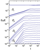
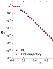
Figure 3: (a) Time evolution of the normalized averaged energies $\overline{E}_{q}(t)/E$, in double logarithmic scale, for the FPU–trajectory arising from the excitation of the first $s=4$ modes with initial conditions $Q_{q}(0)=A_{q}$ if $q=1,2,3,4$ and $Q_{q}(0)=0$ else, and system’s parameters as in Fig.2 for the $q$–torus solution. (b) Comparison of the normalized averaged energy spectra $e_{\kappa}$ versus $\kappa$ of the $q$–torus solution (blue) and the corresponding FPU–trajectory (orange) over a total integration time $T=10^{6}$.

A key feature, now, of the energy transfer process during the first stage of dynamics is the formation of well distinguished groups of modes. Besides the group ${\cal D}_{0}=\{1,2,3,4\}$, which shared the energy initially, by the time evolutions of the energies in Fig.3 we clearly distinguish the groups ${\cal D}_{1}=\{5,6,7,8\}$, ${\cal D}_{2}=\{9,10,11,12\}$ etc, or, in general, ${\cal D}_{k}=\{ks+1,\ldots,(k+1)s\}$. It is observed that, during this stage, for all modes $q$ in the same group ${\cal D}_{k}$, $k>0$ the quantity $\overline{E}_{q}/E$ grows in time by almost the same power–law, i.e. the energy spectra behave as $\overline{E}_{q}(t)/E\sim t^{c_{q}(k)}$, where the exponent is also almost constant within a group: $c_{q}(k)={3\over 2}k+\epsilon_{q}$, with $|\epsilon_{q}|<<1$ for all $q\in{\cal D}_{k}$.

As shown in section 5, the above groups ${\cal D}_{k}$ correspond exactly to the so-called ‘sequence of mode excitations’ associated with a $q$–torus construction via PL series with initial excitation ${\cal D}_{0}$. That is, the sequence of groups formed in the energy transfer process for a FPU-trajectory, during the ‘first stage of dynamics’, coincides with the formal ‘sequence of mode excitations’ appearing in the PL series construction of nearby $q$–tori with the same initial excitation ${\cal D}_{0}$.

It must be emphasized that, in the case of a FPU-trajectory, the separation of the modes into groups is a dynamical phenomenon related to the process of energy transfer. On the contrary, in the case of $q$–tori, the groups only concern a formal aspect of perturbation theory, as analyzed in section 5 below. The fact that the final groups defined in either case are the same, indicates some deeper connection between the $q$–torus solutions and the FPU–trajectories, whose evolution during the first stage of dynamics is integrable-like. Nevertheless, most FPU–trajectories enter eventually into the stage of approach to energy equipartition, whereby their time evolution is weakly chaotic, while the solutions lying on $q$–tori maintain their regular character at all times $t$.

The averaged normalized energy spectrum for the FPU–trajectory at the end of the first stage of dynamics appears to be stabilized to a form persisting for quite long times. This stabilized spectrum exhibits also an exponential profile, very similar to the $q$–torus profile shown in Fig.2(a). The two profiles are superposed in Fig.3(b). We observe that the groups ${\cal D}_{k}$ are well distinguished in the spectrum of the FPU–trajectory, and they coincide with the ones of the $q$–torus solution. To the theoretical interpretation of the latter groups we now turn our attention.

5 Sequence of mode excitations

It is well known that for some special choices of initial conditions, the resulting FPU–trajectories (in both the $\alpha$ and $\beta$ models) take place on lower dimensional invariant sub–manifolds of the FPU phase space. This is due to the existence of discrete symmetries, which give rise to explicit low–dimensional FPU solutions. An extensive study on such symmetries is made in [6, 27, 30] (in the latter such solutions are called ‘bushes of normal modes’). A particular case are periodic trajectories, arising from exciting only one of the modes $q_{0}=N/3$, $N/2$ or $2N/3$ in the $\beta$ model [5] (see also [6, 27]). Solutions like the above lead, by definition, to energy localization, since the energy remains always distributed among a small subset of modes.

On the other hand, as pointed out in the examples of the previous sections, energy localization occurs also for sets of initial conditions not obeying any obvious or simple symmetry. As in [8], we now study this phenomenon using the concept of propagation of some initial excitation in the PL series for low–dimensional tori. We can briefly state our main result as follows: through the study of propagation, we can define a hierarchy of groups of modes participating in a $q$–torus solution, such that all the modes in one group share a similar (in order of magnitude) amount of energy, while distinct groups share quite different amounts of energy. The hierarchy of these groups allows us to predict the whole localization profile via a leading order analysis of the associated PL series. However, as shown in the previous section, it also allows us to characterize the paths of energy transfer in $q$–space for FPU trajectories neighboring some $q$–torus solution, from an initial excitation up to the moment when a metastable profile is established for the FPU–trajectories (like in the example of Fig.3(a)).

We start by the following formal definitions:

Definition 1: A mode $q$ is said to be excited at the $n$–th order of the PL scheme, iff in the series (8) it is $Q_{q}^{(k)}(t)=0$ for all $k<n$, and $Q_{q}^{(n)}(t)\neq 0$. In addition, $Q_{q}^{(n)}(t)$ is called leading order term of the series (8).

Definition 2: Let ${\cal D}_{0}$ be a set of modes excited at the zero order of the PL scheme according to Eqs.(9). The sequence of sets ${\cal D}_{k}$, $k=1,2,\ldots$, where ${\cal D}_{k}$ consists of modes excited at the $k$–th order of the PL scheme, is called sequence of mode excitations.

Definition 3: Let $k_{0}$ be a positive integer. We call tail modes with respect to $k_{0}$ the modes belonging to the set $\cup_{k\geq k_{0}}{\cal D}_{k}$.

Definition 4: We call FPU–trajectory with initial excitation in the set of modes ${\cal D}_{0}\equiv\{q_{1},\ldots,q_{s}\}$ the trajectory resulting from the equations of motion (2) for the set of initial conditions $Q_{q}(0)=A_{q}\cos\phi_{q}$, $P_{q}(0)=-A_{q}\Omega_{q}\sin\phi_{q}$, for some set of amplitudes $A_{q}$ and phases $\phi_{q}$, if $q\in{\cal D}_{0}$, and $Q_{q}(0)=P_{q}(0)=0$ if $q\notin{\cal D}_{0}$.

In order to determine the sequence ${\cal D}_{k}$ produced by a particular initial excitation ${\cal D}_{0}$, we first define the set

$$\Sigma^{r}=\{-1,+1\}^{r}~{}~{}~{}.$$ (16)

The elements of $\Sigma^{r}$ are $r$–dimensional vectors of the form $\sigma^{(r)}=(\sigma_{1},\ldots,\sigma_{r})$, where $\sigma_{i}=1$ or $-1$, $i=1,\ldots,r$. Furthermore, for an $r$–vector $x\equiv(x_{1},\ldots,x_{r})$ we define $\sigma^{(r)}\cdot x$ as the Euclidean product $\sigma^{(r)}\cdot x=\sigma_{1}x_{1}+\ldots+\sigma_{r}x_{r}$. We can now prove the following

Proposition: Let ${\cal D}_{0}=\{q_{1},q_{2},\ldots,q_{s}\}$, $1\leq q_{1}<\ldots<q_{s}\leq N-1$ be the set of seed modes of an initial excitation yielding a formal PL solution associated with trajectories on an $s$–dimensional $q$–torus. Let $M_{k}$ be the set

$$M_{k}=\left\{\Bigg{|}2\left[\frac{\mid\sigma^{(r)}q^{(r)}\mid+N-1}{2N}\right]N-\mid\sigma^{(r)}q^{(r)}\mid\Bigg{|}:\sigma^{(r)}\in\Sigma^{r},~{}~{}q^{(r)}\in{\cal D}_{0}^{r}\right\}$$ (17)

where $r=r(k)$ with $r(k)=k+1$ for the FPU–$\alpha$ model and $r(k)=2k+1$ for the FPU–$\beta$ model. Then, the sequence of mode excitations ${\cal D}_{k}$ corresponding to the initial choice ${\cal D}_{0}$ is defined by the recursive relations

$${\cal D}_{k}=M_{k}\setminus\bigcup_{0\leq j\leq k-1}{\cal D}_{j},~{}~{}k=1,2,\ldots$$ (18)

An explicit proof of the above proposition is given in [8] for the FPU–$\beta$, and in 7 for the FPU–$\alpha$. We note that $\left[\cdot\right]$ is the integer part of a number and $M_{k}$ represents the set of all modes for which the right hand side of Eqs. (3.1) and (3.1) is non–zero, i.e. the modes yielding some non–zero contribution to the energy spectrum up to the $k$–th order of the PL series (some modes excited at previous orders up to $k$ might also belong to $M_{k}$).

Some examples clarify the use of Eq.(18):

i) q–breathers: If we choose ${\cal D}_{0}=\{q_{0}\}$, the so–induced PL solution corresponds to a one–dimensional torus, i.e. a periodic orbit. In this case we find:

$${\cal D}_{k}=\{q_{k}\}~{}\mbox{with}~{}q_{k}=\Bigg{|}2\left[\frac{rq_{0}+N-1}{2N}\right]N-rq_{0}\Bigg{|},$$ (19)

where $r(k)=k+1$ in the FPU–$\alpha$, or $r(k)=2k+1$ in the FPU–$\beta$. This rule coincides with the one given in [15] for an arbitrary seed mode $q_{0}$. From Eq. (19) we readily find that, if $q_{0}$ is even, only even modes become excited at subsequent orders in both the $\alpha$ and $\beta$ models. On the other hand, if $q_{0}$ is odd, in the $\alpha$ model both odd and even modes become excited, while in the $\beta$ model only odd modes become excited. The localization properties of solutions corresponding to $q$–breather excitations will be discussed in detail in Section 6.4 below.

ii) Example with two seed modes: Suppose ${\cal D}_{0}=\{q_{1},q_{2}\}=\{3,5\}$ for $N$ large in FPU–$\alpha$. At first order ($k=1$) it is $r(1)=2$. In order to determine $M_{1}$, we consider all possible combinations of the symbols $\sigma^{(2)}\in\Sigma^{2}$ and $q^{(2)}\in{\cal D}_{0}^{2}$. These are $\{(1,1),(1,-1),(-1,1),(-1,-1)\}$ and $\{(3,3),(3,5),(5,3),(5,5)\}$ respectively. Then from Eq.(17) we find $M_{1}=\{2,3,5,6,8,10\}$. Since ${\cal D}_{0}=\{3,5\}$, from Eq.(18) we have ${\cal D}_{1}=M_{1}\setminus{\cal D}_{0}=\{2,6,8,10\}$. Repeating the above procedure for $k=2$, we find $M_{2}=\{1,3,5,7,9,11,13,15\}$ and ${\cal D}_{2}=M_{2}\setminus{\cal D}_{0}\cup{\cal D}_{1}=\{1,7,9,11,13,15\}$. In the same way we proceed to subsequent orders $k=3,4,\ldots$ In the FPU–$\beta$ one follows the same steps, but for $r(k)=2k+1$.

iii) Excitation representing a low–frequency packet of seed modes: Let us consider as an initial excitation the packet of modes ${\cal D}_{0}=\{1,2,3,4\}$ for $N$ large. Following the same procedure as above, in the FPU–$\alpha$ we find the sequence of excitations ${\cal D}_{1}=\{5,6,7,8\}$, ${\cal D}_{2}=\{9,10,11,12\}$, etc. We notice that at each order modes are excited in groups. In the same way, the $\beta$ model yields ${\cal D}_{1}=\{5,\ldots,12\}$, ${\cal D}_{2}=\{13,\ldots,20\}$, etc.

These propagation rules can be generalized for $s$–dimensional $q$–tori corresponding to low–frequency packets of modes. The seed mode excitation ${\cal D}_{0}=\{1,2,\ldots,s\}$ generates ${\cal D}_{k}=\{ks+1,\ldots,(k+1)s\}$ in the FPU–$\alpha$, and ${\cal D}_{k}=\{(2k-1)s+1,\ldots,(2k+1)s\}$ in the FPU–$\beta$, with $k\geq 1$. Furthermore, we observe that ${\cal D}_{k}^{\beta}={\cal D}_{2k-1}^{\alpha}\cup{\cal D}_{2k}^{\alpha}$. As shown in the next subsection, these rules imply that the resulting $q$–tori solutions exhibit exponential energy localization profiles.

iv) Excitation representing a high–frequency packet of seed modes: As an example, let us consider ${\cal D}_{0}=\{28,29,30,31\}$ in the $N=32$ dimensional chain. In the FPU–$\alpha$ we find ${\cal D}_{1}=\{1,\ldots,8\}$, then ${\cal D}_{2}=\{20,\ldots,27\}$, etc. The general rule, by setting the last $s$ modes ${\cal D}_{0}=\{N-s,\ldots,N-1\}$ as seed modes, is: ${\cal D}_{k}=\{(k-1)s+1,\ldots,(k+1)s\}$, if $k=2n+1$ and ${\cal D}_{k}=\{N-(k+1)s,\ldots,N-(k-1)s-1\}$, if $k=2n$. By the same way, in the FPU–$\beta$ we find ${\cal D}_{k}=\{N-(k+1)s,\ldots,N-(k-1)s-1\}$, $\forall k$. Comparing the two models, we see that ${\cal D}_{k}^{\beta}={\cal D}_{2k}^{\alpha}$.

v) Discrete symmetry solutions: Suppose ${\cal D}_{0}=\{N/2\}$, or ${\cal D}_{0}=\{2N/3\}$. We then find ${\cal D}_{k}={\cal D}_{0}$ for all $k=1,2,\ldots$ in both models, while in FPU–$\beta$ the condition ${\cal D}_{k}={\cal D}_{0}$ holds also for ${\cal D}_{0}=\{N/3\}$. The $q$–breather solutions for these cases correspond to the ‘nonlinear normal modes’ of the FPU system [5, 6, 27], that coincide with the FPU–trajectories resulting from the same seed mode.

We note finally, that for $q$–breathers we have a general relation connecting the sequences of excitations ${\cal D}_{k}$ in the $\alpha$ and in the $\beta$ model, starting from the same seed mode. Namely, from Eq.(19) we find that ${\cal D}_{k}^{\beta}={\cal D}_{2k}^{\alpha}$. In words, the mode excited at the $k$–th order in the FPU–$\beta$ is the same as the mode excited at the $2k$–th order in the FPU–$\alpha$. This relation holds also for excitations of small packets around $N/4$, $N/2$ and $3N/4$, but it does not hold in the case (iii) (low-frequency packets of modes). In fact, for an arbitrary excitation we have $M^{\alpha}_{2k}=M^{\beta}_{k}$, but we only have ${\cal D}_{k}^{\beta}={\cal D}_{2k}^{\alpha}$ provided that $M^{\alpha}_{2k-1}\cap M^{\alpha}_{2k}=\emptyset$.

6 Numerical examples. Localization profiles

In this section we provide various numerical tests on the energy profiles and dynamics of the $q$–tori and their neighboring FPU–trajectories. We are interested to examine several generic localizations profiles, rising by the excitation of arbitrary modes, consecutive or isolated, that form different localization patterns in $q$–space. In particular, we derive the precise sequence of modes that become excited in subsequent orders by $s$ consecutive modes, chosen to be in the i) beginning, ii) one fourth, iii) middle and iv) three fourths of the spectrum, while in case i) we predict the localization law of the energy profile. Finally, few examples on $q$–breathers, as particular cases of one dimensional $q$–tori, are given.

The frequencies and amplitudes used throughout all examples below are listed in 7.

6.1 $q$–Tori low frequency packet solutions and exponential energy localization

The FPU–trajectory examined in Section 4 is an example of a class of solutions of particular interest in the literature (see [2, 3, 4, 26]), namely solutions corresponding to the initial excitation of a packet of low–frequency modes. In fact, it is numerically found that, for values of the specific energy beyond some threshold, low–frequency packets of modes are formed naturally, even if initially we excite only one, e.g. the $q=1$ mode. Some questions of central interest in the literature concern the dependence of: i) the width of natural packets and ii) the exponential slope of the energy spectrum of the remaining modes, on system’s parameters $E$, $N$ etc (see [23] for a review).

In the sequel we examine the form of localization profiles for $q$–torus solutions associated with an initial excitation of a low–frequency packet of modes. We obtain theoretical results based on a leading order term analysis of the PL series for $q$–tori (see 7). Furthermore, we compare these results with ones found numerically for FPU–trajectories with a similar initial excitation.

6.1.1 FPU–$\alpha$ model

Our main result for the FPU–$\alpha$ can be stated as follows: in Section 5 it was mentioned that, for $q$–tori, an initial excitation ${\cal D}_{0}=\{1,2,\ldots,s\}$ in the PL series leads to the sequence of mode excitations ${\cal D}_{k}=\{ks+1,\ldots,(k+1)s\}$. Starting, now, from the median mode in the group ${\cal D}_{k}$, i.e. the mode $q_{mid}=ks+[{s}/{2}]$, we can obtain estimates of the size of the leading term $Q_{q_{mid}}^{(k)}$ given by Eq.(32) and derive estimates on the magnitude of the harmonic energy $E_{q_{mid}}^{(k)}$, which is hereafter denoted by $E^{(k)}$. Then, we find:

$$E^{(k)}\simeq\frac{(k+1/2)^{2}\varepsilon}{M}\left(\frac{\alpha^{2}N^{4}\varepsilon}{\pi^{4}s^{4}}\right)^{k}$$ (20)

where $M=s/N$ is the fraction of initially excited modes with respect to the total number of modes. The derivation of Eq. (20) is given in 7.

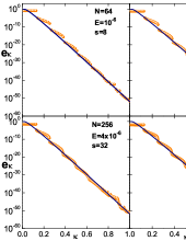
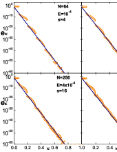
Figure 4: Normalized averaged energy spectra $e_{\kappa}$ versus $\kappa$ for FPU–trajectories (orange spheres) in both the FPU–$\alpha$ and FPU–$\beta$ models, keeping the specific energy $\varepsilon$ and the ratio of initially excited modes $M$ fixed. The parameters are: (a) FPU–$\alpha$ model with $\alpha=0.33$, $M=1/8$, $\varepsilon=1.5625\times 10^{-8}$. (b) FPU–$\beta$ model with $\beta=0.3$, $M=1/16$ and $\varepsilon=1.5625\times 10^{-6}$. In (a), the blue line in all panels corresponds to the theoretical prediction of Eq.(21) based on the leading order term analysis for $q$–tori. This is given by $\log e_{\kappa}=-56.27\kappa+4.46+2\log\kappa$. In (b) the blue line corresponds to a similar prediction for the FPU–$\beta$, given by Eq.(23). We find $\log e_{\kappa}=-78.64\kappa-1.204$.

Normalizing Eq.(20) we obtain an equivalent expression for $e_{\kappa}=E^{(k)}/E$

$$\log e_{\kappa}\simeq\frac{\log\lambda}{M}\kappa+2\log\kappa-\log(\lambda^{1/2}M^{3}N)$$ (21)

where $\kappa=q/N$ is re–scaled wavenumber and $\lambda=\alpha^{2}\varepsilon/\pi^{4}M^{4}$. The main prediction is that if $\alpha,\varepsilon$, and the fraction $M=s/N$ are kept fixed, the normalized energy profiles of $q$–tori remain unaltered as $N$ increases.

This prediction becomes hardly possible to test by a direct construction of the $q$–tori solutions via PL series, because as $N$ increases, we quite soon encounter the limits of computer memory required for storing the coefficients produced by the computer–algebraic program. However, taking into account the evidence presented in subsection 4.1, that FPU–trajectories with the same initial excitations as $q$–tori exhibit similar localization profiles, we can test numerically the extent up to which the invariance of the averaged normalized energy spectrum holds, at least for FPU–trajectories.

Such a test is made in Fig.4. In (a) we give the normalized averaged energy spectrum $e_{\kappa}$ as a function of the re–scaled wavenumber $\kappa=q/N$ for an FPU–trajectory of $\alpha=0.33$, $M=1/8$, and $\varepsilon=1.5625\times 10^{-8}$. We computed these trajectories by progressively increasing $N$, namely $N=64$, $128$, $256$ and $512$. The energy spectra of Fig.4 are all evaluated at $T=10^{6}$. The solid line corresponds to the fitting law of Eq. (21), which, for the adopted parameters, takes the form indicated in the figure caption. The main remark is that the same line fits all re–scaled normalized spectra, for different $N$ (while the fraction of initially excited modes $M=1/8$ as well as the specific energy $\varepsilon=1.5625\times 10^{-8}$ are kept constant).

A relevant question of central interest regards the upper limit in the specific energy for which the normalized spectra for the FPU–trajectories continue to exhibit exponential localization. Eq.(20) allows us to obtain an upper limit, by requiring that $\lambda=\alpha^{2}\varepsilon/\pi^{4}M^{4}<1$. However, as we approach the upper limit $\varepsilon=\pi^{4}M^{4}/\alpha^{2}$, the analysis based on only the leading order terms of the PL series ceases to be valid, since important contributions to the energy spectrum are made also by the higher order terms in each mode’s series expansion of Eq.(8).

The condition $\lambda<1$ implies $s>\alpha^{1/2}\varepsilon^{1/4}N$. Thus Eq.(20) applies when the initially excited packet has a width larger than the width of the so–called natural packets [2, 3, 4]. In the case of natural packets, it is found that by the excitation of a number of low frequency modes satisfying $s<\alpha^{1/2}\varepsilon^{1/4}N$, the so resulting energy spectrum exhibits a plateau of width $\alpha^{1/2}\varepsilon^{1/4}N$ (larger than the initially excited modes). Furthermore, there is evidence that the slope $\tilde{\sigma}$ of the exponential energy localization profile $e_{\kappa}\sim\exp(-\tilde{\sigma}\cdot\kappa)$ depends linearly on $\alpha^{-1/2}\varepsilon^{-1/4}$ [28]. This is in contrast to the slope which refers to $q$–tori solutions of Eq.(20), that depends logarithmically on $[\alpha^{-1/2}\varepsilon^{-1/4}]^{-4}$ and points out that different choices in the fraction of the initially excited low–frequency modes result in different exponential laws.

6.1.2 FPU–$\beta$ model

For the sake of completeness we report the results of our previous work [8], concerning exponential energy localization in the FPU–$\beta$ model. Assuming the initial excitation to be ${\cal D}_{0}=\{1,2,\ldots,s\}$, the sequence of mode excitations in the PL series at the orders $k=1,2,\ldots$ is ${\cal D}_{k}=\{(2k-1)s+1,\ldots,(2k+1)s\}$. Estimating the size of the median mode $q_{mid,k}=2ks$ in each group ${\cal D}_{k}$ via Eq.(32), we are lead to an estimate for the energy spectra of $q$–tori with the above excitation, namely

$$E^{(k)}\simeq{\varepsilon\over M}\left({\beta^{2}\varepsilon^{2}\over\pi^{4}M^{4}}\right)^{k}~{}~{}$$ (22)

where $M=s/N$. Using re-scaled variables as in the $\alpha$ case, Eq.(22) takes the form

$$\log e_{\kappa}\simeq\frac{\log\lambda}{M}\kappa-\log s$$ (23)

where $\lambda={\beta\varepsilon/\pi^{2}M^{2}}$. We find a similar result as in the $\alpha$ case, namely Eq.(23) implies that by keeping both the specific energy $\varepsilon$ and the fraction of excited modes $M$ fixed, while $N$ increases, the normalized exponential profile remains invariant. Again, in order that the analysis be valid, one must have $s>N(\beta\varepsilon)^{1/2}$, implying that the initial excitation should be in a regime quite different from that of natural packets. In fact, in the present case as well, Eq.(23) describes correctly the localization profile provided that $\lambda<<1$ (see also [8]).

As a numerical test of the above predictions we use again numerical computations based on FPU–trajectories rather than exact $q$–tori solutions. The four panels of Fig.4(b) show the normalized averaged spectra $e_{\kappa}$ of FPU–trajectories, along with the predictions of Eq.(23), for the fixed values $M=s/N=1/16$, and $\varepsilon=1.5625\cdot 10^{-6}$. We observe again that the spectrum remains practically invariant with increasing $N$.

6.2 Localization patterns for arbitrary initial excitations

So far, we focused on $q$–tori, and their neighboring FPU–trajectories corresponding to initial excitations in the low–frequency part of the spectrum. However, it is possible to see that energy localization appears also in cases where the initial excitation has quite different features than in the case of packets of low–frequency modes. In particular, we will examine now $q$–tori solutions in the FPU–$\alpha$ system produced by an initial excitation ${\cal D}_{0}$ consisting of a small set of $s$ modes arbitrarily distributed in $q$–space. We give several such examples, in which we vary $s$, $N$, $E$, as well as ${\cal D}_{0}$. As in the example of Fig.2(a), in all present cases we compare the averaged normalized energy spectra $e_{\kappa}^{PL}$ obtained with the PL series, with the ones $e_{\kappa}^{PLn}$ obtained by numerical integration of the equations of motion for the initial conditions $Q_{q}^{PL}(0)$, $P_{q}^{PL}(0)$, $q=1,\ldots,N-1$.

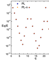
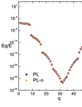
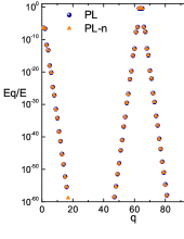
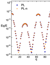
Figure 5: Normalized averaged energy spectra $E_{q}$ versus $q$, deduced by the PL series $q$–torus solution (blue spheres), or a numerical integration (PLn) with initial conditions on a $q$–torus (orange triangles, see text). (a) $N=32$, $\alpha=0.33$, ${\cal D}_{0}=\{1,11,21,31\}$, (b) $N=64$, $\alpha=1$ with ${\cal D}_{0}=\{60,61,62,63\}$. (c) $N=128$, $\alpha=1$ with ${\cal D}_{0}=\{63,64,65\}$. (d) $N=128$, $\alpha=1$ and ${\cal D}_{0}=\{94,95,96,97,98\}$. The chosen frequency values, and resulting amplitudes and energies in each case are given in 7.

Example 1: evenly distributed initial excitation. In the FPU–$\alpha$ with $N=32$, we construct a $q$–torus PL series starting from the 0–th order excitation ${\cal D}_{0}=\{1,11,21,31\}$, when the frequency values for $\omega_{1}$, $\omega_{11}$, $\omega_{21}$, $\omega_{31}$ are chosen as in the second group of 7. The truncation order here is $k_{0}=11$. Solving numerically Eqs.(10) we specify the values of the amplitudes $A_{1}$, $A_{11}$, $A_{21}$ and $A_{31}$. The total energy is $E=0.001563$.

Fig.5(a) shows the averaged normalized energy spectrum for the above $q$–torus solution. Energy localization is manifestly present, since we observe the formation of four peaks of the energy spectrum around the seed modes 1,11,21 and 31. The localization pattern is readily understood by computing the sequence of mode excitations ${\cal D}_{k}$ deduced by the proposition of Section 5. Namely, we find ${\cal D}_{1}=\{2,10,12,20,22,30\}$, ${\cal D}_{2}=\{3,9,13,19,23,29\}$, ${\cal D}_{3}=\{4,8,14,18,24,28\}$, ${\cal D}_{4}=\{5,7,15,17,25,27\}$ etc. We observe that consecutive modes, adjacent (on either side) to the initially excited ones, are excited at subsequent orders of perturbation theory. Thus, starting for example from the mode $q=11$, the modes $q=10,12$ are excited at first order, $q=9,13$ at second order, etc. This explains the formation of the peaks in the spectrum. In fact, the pairs $\{10,12\}$, $\{9,13\}$, etc. share quite similar energies, corresponding to excitation amplitudes $O(\mu)$, $O(\mu^{2})$, $\ldots$ As a result, the local form of the energy spectrum on either side of one peak is exponential.

Finally, as evident in Fig.5(a), we find a very precise agreement between the normalized spectrum corresponding to the analytical solution $Q_{q}^{PL}(t)$, and the one $Q_{q}^{PLn}(t)$ obtained by numerical integration of the initial conditions on the $q$–torus. This fact indicates that at the truncation order $k_{0}=11$ the solution has converged to a good accuracy.

Example 2: initial excitation in the high–frequency part of the spectrum. We consider a $q$–torus solution found by PL series in the case $N=64$, $\alpha=1$, when ${\cal D}_{0}=\{60,61,62,63\}$, while the choice in the frequencies and the resulting amplitudes are shown in the third group of 7. The truncation order of the series is $k_{0}=8$ and the energy is $E=0.000883$.

Fig.5(b) shows the resulting averaged normalized energy spectrum for the above $q$–torus solution. This displays several features similar to the case of a low–frequency excitation. Namely, we observe the formation of groups of consecutive modes sharing a similar amount of energy. The sequence of mode excitations in this case turns out to be ${\cal D}_{1}=\{1,\ldots,8\}$, ${\cal D}_{2}=\{52,\ldots,59\}$, ${\cal D}_{3}=\{9,\ldots,16\}$, ${\cal D}_{4}=\{44,\ldots,51\}$, etc.

Finally, we note again the exponential fall of the energy along two separate branches of the spectrum, namely a low–frequency and a high–frequency branch.

Example 3: excitation in the middle part of the spectrum. We consider the middle modes initial excitation ${\cal D}_{0}=\{63,64,65\}$ in the FPU–$\alpha$ with $\alpha=1$, $N=128$, and with frequencies and amplitudes displayed in the fourth group of 7. The PL series are truncated at $k_{0}=16$ and the energy of the system is $E=7.63469\times 10^{-5}$.

In the averaged normalized energy spectrum $E_{q}^{PL}/E$ (Fig.5(c)) we observe that three energy peaks are formed: by the lowest, the highest and the middle modes. The spectrum of our numerical solution $E_{q}^{PLn}/E$ follows $E_{q}^{PL}/E$ until values of the order $10^{-60}$. We find that the sequence of mode excitations here is ${\cal D}_{1}=\{1,2,126,127\}$, ${\cal D}_{2}=\{61,62,66,67\}$, ${\cal D}_{3}=\{3,4,124,125\}$, ${\cal D}_{4}=\{59,60,68,69\}$, etc.

Example 4: excitation in the 3/4 part of the spectrum. We consider, as before, $N=128$, $\alpha=1$, and an initial excitation ${\cal D}_{0}=\{94,95,96,$ $97,98\}$. The chosen frequency values and the so–resulting amplitudes are shown in the fifth group of 7. The truncation order is $k_{0}=9$ and the energy is $E=0.000649478$.

At subsequent orders, we now find the sequence of mode excitations ${\cal D}_{1}=\{1,2,3,4\}\cup\{60,\ldots,68\}$, ${\cal D}_{2}=\{26,\ldots,38\}\cup\{90,\ldots,93\}\cup\{99,\ldots,102\}$, ${\cal D}_{3}=\{5,\ldots,8\}\cup\{56,\ldots,72\}\cup\{120,\ldots,127\}$, ${\cal D}_{4}=\{22,\ldots,25\}\cup\{39,\ldots,42\}$ $\cup\{86,\ldots,89\}\cup[103,\ldots,106\}$, etc. This leads to the localization pattern shown in Fig.5(d).

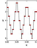
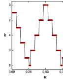
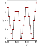
Figure 6: Propagation of modes for an initial excitation ${\cal D}_{0}=[\kappa_{0}-\epsilon,\kappa_{0}+\epsilon]$ when (a) $\kappa_{0}=1/4$, (b) $\kappa_{0}=1/2$ and (c) $\kappa_{0}=3/4$. In all panels, the ordinate yields the order $k$ of perturbation theory at which the (re–scaled) mode $\kappa=q/N$ is first excited. Since in the exponential energy localization regime we always have $\log e_{\kappa}\sim\kappa$, the patterns shown in the present panels are similar to the energy spectra for the same excitations plotted in semi–logarithmic scale.

6.3 Patterns from generalized packet excitation

We now generalize results on the localization patterns formed by initial excitations of packets of arbitrary width, around the locations in $q$–space corresponding the one fourth, half and three thirds of the spectrum. We suppose that each packet is of the form ${\cal D}_{0}=[\kappa_{0}-\epsilon,\kappa_{0}+\epsilon]$, having a width equal to $s/N=2\epsilon$, $\epsilon<<1$ in the normalized $q$–space $\kappa=q/N\in[0,1]$. In order to specify the sequence of mode excitations ${\cal D}_{k}$ at subsequent orders, we first specify the sets $M_{k}$ defined in Eq.(17), whereby the sets ${\cal D}_{k}$ are immediately derived by the relation ${\cal D}_{k}=M_{k}\setminus\cup_{0\leq j\leq k-1}M_{j}$. Examining in detail the case of excitations around the re–scaled wavenumbers $\kappa_{0}=1/4$, $1/2$, or $3/4$ we have:

1) For $\kappa_{0}=1/4$ we find $M_{k}=[0,\epsilon(k+1)]\cup[1/2-\epsilon(k+1),1/2+\epsilon(k+1)]\cup[1-\epsilon(k+1),1]$, if $k=2n+1$ and $k>1$, or $M_{k}=[1/4-\epsilon(k+1),1/4+\epsilon(k+1)]\cup[3/4-\epsilon(k+1),3/4+\epsilon(k+1)]$, if $k=2n$. Only the case of $k=1$ differs, for which it turns out that $M_{1}=[0,2\epsilon]\cup[1/2-2\epsilon,1/2+2\epsilon]$, i.e. the last modes are not yet excited. The resulting localization pattern displays three peaks around $\kappa=0$, $1/2$, and $1$, produced at odd orders, and two peaks around $1/4$ and $3/4$, produced at even orders. The total pattern is shown in Fig.6(a). In this figure, the ordinate in all panels indicates the order $k$ of the PL series at which the corresponding mode, of wavenumber $\kappa=q/N$, is first excited. In fact, according to the leading order term analysis of the PL series discussed above we have $\log e_{\kappa}\sim\kappa$. Thus, the patterns shown in all panels of Fig.6 are similar to the averaged normalized energy spectra for the corresponding excitations when plotted in semi–logarithmic scale.

2) For $\kappa_{0}=1/2$ we find $M_{k}=[0,\epsilon(k+1)]\cup[1-\epsilon(k+1),1]$, if $k=2n+1$, or $M_{k}=[1/2-\epsilon(k+1),1/2+\epsilon(k+1)]$, if $k=2n$. Thus, we have two localization peaks around $\kappa=0$ and $\kappa=1$ created by contributions at odd orders of the PL series, and one more peak around $\kappa=1/2$ for contributions at even orders. The overall localization pattern is shown in Fig.6(b).

3) For $\kappa_{0}=3/4$ we find similar results as in case (1), i.e. $M_{1}$ is $[0,2\epsilon]\cup[1/2-2\epsilon,1/2+2\epsilon]$ and then $M_{k}=[0,\epsilon(k+1)]\cup[1/2-\epsilon(k+1),1/2+\epsilon(k+1)]\cup[1-\epsilon(k+1),1]$, if $k=2n+1$ and $k>1$, and $M_{k}=[1/4-\epsilon(k+1),1/4+\epsilon(k+1)]\cup[3/4-\epsilon(k+1),3/4+\epsilon(k+1)]$, if $k=2n$. In fact, the only difference with respect to case (1) concerns the initial excitation at the order $k=0$. The resulting localization pattern is shown in Fig.6(c).

6.4 $q$–breathers and FPU–trajectories

The existence, stability, and energy localization properties of $q$–breathers were studied extensively in [11]–[15], [21], [22]. It was found that $q$–breathers have quite similar energy localization profiles as their nearby FPU–trajectories. Furthermore, the $q$–breathers are periodic orbits whose existence, for an arbitrarily high energy, is guaranteed by the Lyapunov’s theorem. Therefore, their existence extends well beyond the domain of convergence of their associated PL series.

However, the PL series can still be quite useful in studying analytically some properties of $q$–breathers. In the sequel we examine $q$–breathers as a particular case of one–dimensional $q$–tori. A computational advantage is that, at any fixed order $k$, the number of terms in the resulting series is substantially smaller for $q$–breathers than for $q$–tori of any other dimension $s>1$. This fact allows us to construct the series up to a very high order (in the case $N=32$ we were able to compute examples of PL series for $q$–breathers up to the truncation order $k_{0}=250$). Even so, the convergence of the resulting series is very slow, and in practice we obtain little gain in precision after a truncation order near $k_{0}=50$. In most of our trial examples, the precision achieved for the computation of initial conditions on a $q$–breather using PL series is 4 to 6 significant digits, while in some cases we reach 10 significant digits. However, using these numbers as initial guess, we are able to determine many more via a root–finding technique. Let us note that a root-finding determination is possible only in the case of $q$–breathers, which are periodic orbits, while we cannot use such technique in the case of $q$–tori of dimension higher than one.

6.4.1 The breather $q=1$

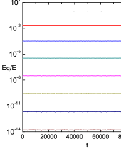
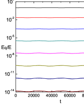
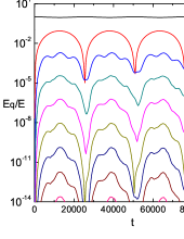
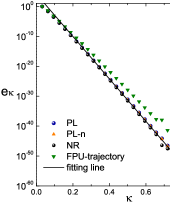
Figure 7: FPU–$\alpha$ system with $\alpha=0.33$, $N=32$ and $E=0.00016635$. In Panels (a), (b) and (c) is shown the evolution of the normalized instantaneous spectra $E_{q}(t)/E$ of modes $q=1,\ldots,8$ for the PL solution, the numerical integration of FPU–dynamics for the same initial conditions with (a) and for the FPU–trajectory with seed mode $q=1$, respectively (the energy $E_{q}$ has the highest value for $q=1$ and it progressively decreases for $q=2,3,\dots$). In panel (d) is the exponential profile of the normalized averaged energy spectra $e_{\kappa}$ versus $\kappa$ of panel (a) with blue spheres, of (b) with orange triangles, of (c) with green triangles, as well as the $q$–breather found by Newton–Raphson (NR) with black spheres. The continuous line is the fitting law (24).

As a first example, we consider the construction of a $q$–breather with ‘seed mode’ $q_{0}=1$. The sequence of mode excitations here is $q_{k}=k+1$. Fig.7 refers to a calculation for $N=32$, $\alpha=0.33$ and $E=0.00016635$, for the truncation order $k_{0}=51$. The choice of $\omega_{1}$, as well as the resulting amplitude $A_{1}$, are given in 7. As for the overall precision in the analytic determination of the periodic orbit using PL series at the truncation order $k_{0}=51$, we find that this trajectory returns to its initial conditions after the time $T=2\pi/\omega_{1}$, with $\omega_{1}$ specified by the PL method, up to 10 significant digits, or more using the values $Q_{q}^{PL,51}(0),P_{q}^{PL,51}(0)$ as initial guess values for a numerical (Newton–Raphson) determination of the periodic orbit.

Fig.7(a),(b) and (c) show the evolution of the normalized harmonic energies $E_{q}(t)/E$, for $q=1,\ldots,8$ in three different computations. Namely, in (a) we compute $E_{q}(t)$ by the analytical solution $Q_{q}^{PL,51}(t)$ as found by the truncated PL series. In (b), we integrate numerically the initial conditions $Q_{q}^{PL,51}(0)$, $P_{q}^{PL,51}(0)$. Finally, in (c) we consider a FPU–trajectory rising by the simple initial condition (corresponding to $q_{0}=1$): $x_{n}(0)=A_{1}\sin(\pi n/N)$, $y_{n}(0)=0$, $n=1,\ldots,N-1$.

The main remark, by a direct comparison of the three panels, is an important difference in the temporal behavior of the $q$–breather (in Fig.7 (a) and (b)) from that of the corresponding FPU–trajectory (Fig.7 (c)). Namely, the energies $E_{q}(t)$, $q=1,\ldots,8$ remain practically constant in the case of the $q$–breather, while they behave as quasi–periodic functions in the case of the FPU–trajectory. In fact, the energies $E_{q}(t)$ for the latter oscillate around mean values following closely the energy values of the $q$–breather solution, but with an amplitude causing variations of more than one orders of magnitude.

Fig.7(d) shows a comparison of the averaged normalized energy spectra in all four computations, namely (i) $Q_{q}^{PL,51}(t)$, (ii) $Q_{q}^{PLn,51}(t)$, (iii) the FPU–trajectory, and (iv) the periodic orbit with initial conditions as determined by the Newton–Raphson. The solid line in Fig.7(d) corresponds to the exponential law

$$E_{q}=\gamma^{q-1}q^{2}E_{1},~{}~{}where~{}~{}\gamma=\alpha^{2}N^{4}\varepsilon/\pi^{4},$$ (24)

suggested as a fitting law in [12].

6.4.2 The breather $q=25$

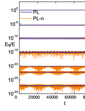
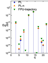
Figure 8: FPU–$\alpha$ system with $\alpha=0.33$, $N=32$, $E=0.00465079$ with seed mode $q_{0}=25$. In panel (a) it is shown the evolution of the normalized instantaneous spectra $E_{q}(t)/E$ of modes $25,14,11,28,3,22,17$ for the PL solution of the $q$–breather (blue) and the numerical integration (PLn) of the initial condition $Q_{q}^{PL}(0)$, $P_{q}^{PL}(0)$ (orange). In panel (b) is the exponential profile of the normalized averaged energy spectra $\overline{E}_{q}/E$ versus $q$ of PL with blue spheres, of PLn with orange triangles and of the FPU–trajectory with green triangles.

Fig.8 refers, now, to a different $q$–breather example, in which we choose to initially excite a mode at an arbitrary position in $q$–space, namely $q_{0}=25$, for the system with $\alpha=0.33$, $N=32$ and $E=0.00465079$. Again $\omega_{25}$ and $A_{25}$ are found in the table of 7, while the truncation order here is $k_{0}=60$. The sequence of mode excitations derived from Eq.(19) up to the $10$–th order of perturbation theory is $q_{1}=14$, $q_{2}=11$, $q_{3}=28$, $q_{4}=3$, $q_{5}=22$, $q_{6}=17$, $q_{7}=8$, $q_{8}=31$, $q_{9}=6$, and $q_{10}=19$.

Fig.8(a) shows the temporal evolution of the normalized energies $E_{q}(t)/E$ of the first seven modes in the sequence of excitations, namely $q_{0},\ldots,q_{6}$, for the solutions $Q_{q}^{PL,60}(t)$ (blue) and $Q_{q}^{PLn,60}(t)$ (orange). Differences observed between the energy spectra which are below $10^{-15}$ show that the numerical integration cannot preserve precisely the analytical construction and therefore the energy spectra make some small oscillations.

Fig.8(b) now shows the normalized averaged spectra for the solutions (i) $Q_{q}^{PL,60}(t)$, (ii) $Q_{q}^{PLn,60}(t)$, and (iii) a FPU–trajectory rising by the seed mode excitation $q_{0}=25$. We clearly see again that the FPU–trajectory’s spectrum deviates from the $q$–breather’s one at modes corresponding to a higher order in the excitation sequence. Still, however, the hierarchy of modes in the energy spectrum is preserved.

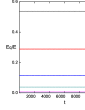
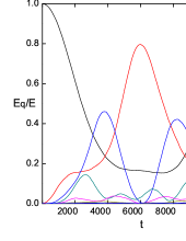
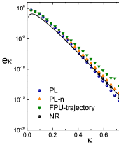
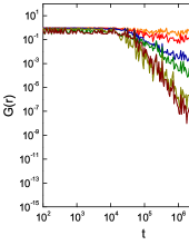
Figure 9: FPU–$\alpha$ with $N=32$, $\alpha=0.33$, $E=0.014915$ and seed mode $q_{0}=1$. Panels (a) and (b) are for the evolution of the normalized instantaneous spectra $E_{q}(t)/E$ for the $q$–breather and the FPU–trajectory, respectively. In panel (c) is the exponential profile of the normalized averaged energy spectra $e_{\kappa}$ of PL with blue spheres, the numerical integration (PLn) of the initial condition $Q_{q}^{PL}(0)$, $P_{q}^{PL}(0)$ with orange triangles, of FPU–trajectory with green triangles and of NR with black spheres. The continuous line is the fitting law (24). In (d) is the evolution of the GALI indices $G_{2},G_{3},\ldots,G_{7}$.

6.4.3 The original FPU–trajectory: how many frequencies?

We finally discuss a FPU–trajectory similar to the classical experiment of Fermi Pasta and Ulam in [10], leading to the observation of the celebrated FPU–recurrences (Fig.9(b)). Practically, we return to the example of Subsection 6.4.1, but for a higher energy. The PL construction of the corresponding $q$–breather to this FPU–trajectory was made for $E=0.014915$ and truncation order $k_{0}=242$ ($\omega_{1}$ and $A_{1}$ are given in 7).

Comparing their energy spectra in Fig.9(c), we see a quite good agreement, especially to the low–frequency modes. While these two objects are lying close in phase space, we would like to emphasize that they exhibit a different dynamical behavior. It can be observed, from the temporal evolution of their energy spectra, that the case of the FPU–trajectories shown in Fig.9(b), contrary to the almost constant $q$–breather’s spectra of Fig.9(a), clearly show a recursive behavior, leading to a nearly complete return to their initial values at the time $t=12000$.

By implementing the GALI method, we find that the number of incommensurable frequencies that govern this FPU–trajectory is five, a fact implying that it lies on a 5–dimensional torus. In particular, Fig.9(d) shows that the indices $G_{2}$ and $G_{3}$ are constant from the beginning, while $G_{4}$ and $G_{5}$ reach an asymptotic constant value at nearly $t=5\times 10^{7}$, giving evidence for a 5–dimensional torus with 3 dominant actions and 2 compactified in smaller scales.

We note, in this latter respect, that according to [4], an excitation as in Fig.9 should lead to the formation of a ‘natural packet’ of modes exhibiting a sort of internal equipartition. However, the prediction for the packet width yields $\alpha^{1/2}\varepsilon^{1/4}N\simeq 2.7\simeq 3$, which is smaller than the dimension of the torus as suggested by the GALI indicators. On the other hand, a very recent study by Genta et al. [18] shows that the cutoff of the packet’s width is proportional to $a^{2/5}\varepsilon^{1/5}N\simeq 4.43$ (between 4 and 5).

We thus conclude that the dynamics of the FPU trajectory of Fig.9(b) shares a number of common features with a $q$–breather with a similar initial excitation, but also a number of common features with low–dimensional objects of dimension higher than one. In fact, the numerical indications are that the dimension of the associated object is around 5. However, in the present case the energy is quite high and our attempt to construct a torus solution analytically does not appear to lead to a convergent PL series. We thus leave open for future study the question of truly separating between solutions of different dimension that approximate the dynamics of FPU trajectories in this regime.

7 Conclusions

In the present paper, we study the dynamical features and localization properties of low–dimensional invariant objects of the FPU phase space called $q$–tori. Our main findings can be summarized as follows:

1) We use the method of Poincaré – Lindstedt (PL) series in order to compute quasi-periodic series representations of trajectories approximating the motion on $q$–tori, up to a high order in a small parameter. We give some details on the way by which appropriate values of the torus frequencies are chosen in order for the PL method to proceed. We also test numerically the convergence behavior of our PL series. In particular we show that our series exhibit the phenomenon of cancellations between terms of a big size, leaving a small residual. Furthermore, the GALI indicator was used as an additional test for verifying the dimension of our computed $q$–tori solutions.

2) Using properties of the PL series construction, we study the phenomenon of energy localization on $q$–tori. We present a theory of propagation of initial ‘excitations’ in the series terms. Via this theory we predict theoretically the form and shape of energy localization profiles for $q$–tori. Finally, we compare the latter with the energy localization profiles of orbits lying in the neighborhood of $q$–tori (called ‘FPU–trajectories’).

3) Regarding the FPU–trajectories lying in the neighborhood of $q$–tori solutions, we find that they exhibit energy localization phenomena leading to an averaged normalized energy spectrum tending to saturate to a form quite close to that of a $q$–torus solution with similar initial excitation. We provide numerical evidence that the so–called ‘first stage’ in [29] of energy transfer in FPU–trajectories, involves energy transfer among groups defined by the sets ${\cal D}_{k}$, as in the $q$–tori case. A theoretical interpretation of this phenomenon remains an open question.

4) As a case of particular interest, we study low–frequency packet excitations. In this case, we show that $q$–tori solutions predict the appearance of exponential localization profiles, with a slope depending logarithmically on the specific energy of the system and on the percentage of the modes excited. Thus, the normalized energy spectra are invariant with respect to the re–scaled wavenumber $\kappa=q/N$, as long as the fraction of modes excited $s/N$ and the specific energy are kept constant. Via leading order estimates in the PL series, we derive a law for the slope of the exponential energy profile, both in the FPU–$\alpha$ and FPU–$\beta$ models. This turns out to be similar to that of $q$–breather solutions in which the ‘seed mode’ $q_{0}$ is allowed to vary proportionally to $N$. In fact, such laws suggest the invariance of the $q$–tori’s localization profiles as we approach the thermodynamic limit, provided that $s/N$ and specific energy $\varepsilon$ are kept constant. However, the existence of $q$–tori as $N\rightarrow\infty$ is still an open issue, as we have no proof of the convergence of the PL series in a finite domain of initial conditions as we approach this limit.

5) Excitations of packets of consecutive modes not in the low frequency part of the spectrum lead to non–trivial localization profiles that have not been extensively studied in the literature. A study of the FPU–trajectories arising from such initial conditions, as well as of the times needed for such trajectories to reach equipartition, is an interesting open problem.

6) The computer–algebraic program of the PL series presently used for the determination $q$–tori was employed also in the case of $q$–breathers, leading to high precision calculations corresponding to orders of the PL series higher than $k=60$. Using also our algorithm of systematic determination of frequencies (7), we are able to locate $q$–breathers of quite high energy values. We find that, as the energy of the system increases, the distance between $q$–breathers and FPU–trajectories resulting from the same initial excitation also grows. Furthermore, the FPU–trajectories exhibit a dynamics consistent with an increasing number of incommensurable frequencies. Nevertheless, the spectra of the FPU–trajectories remain strongly localized in $q$–space.

As a final remark, we note that the time for which ‘metastable states’ of FPU–trajectories started close to $q$–tori persist, as well as its dependence on the system’s parameters, is an interesting open question that can be considered as complementary to the study in [2] (where the initially excited packet is smaller than the natural one). This is proposed as a subject for future study.

Acknowledgments

We wish to thank A. Ponno and G. Benettin for their useful discussions clarifying particular points of the paper. H.C. gratefully acknowledges the hospitality of the Dipartimento di Matematica Pura e Applicata, Universitá di Padova, during the period May 2010 to May 2012, where this work was initiated and completed.

APPENDIX

A. Algorithm of determination of frequency values for the PL series construction

We give an iterative algorithm of determination of numerical values of the frequencies $\omega_{q_{i}}$, $q_{i}\in{\cal D}_{0}$, for a $q$–torus solution with initial excitation ${\cal D}_{0}$, such that the solution constructed at every step corresponds to a higher specific energy than the solution constructed in the previous step. The algorithm consists of the following steps:

Initialization. i) We choose some value of ‘trial amplitudes’ $A_{q_{i}}^{trial}$ and define

$$\epsilon_{l,trial}={1\over N}\sum_{i=1}^{s}{1\over 2}\Omega_{q_{i}}^{2}A_{q_{i},trial}^{2},~{}~{}q_{i}\in{\cal D}^{(0)}~{}~{},i=1,\ldots s.$$ (25)

ii) We compute ‘trial’ frequencies by the lowest-order frequency correction terms in the series (10) corresponding to the trial amplitudes $A_{q_{i},trial}$.

In the FPU-$\alpha$ the frequencies $\omega_{q_{i}}$ appear in the denominators of the lowest order terms, we implement a two-step substitution-iteration procedure. Namely we set

$$\omega_{q,mid}^{(2)} = -\frac{\Omega_{q}}{4}\sum_{\mathop{m\in{\cal D}^{(0)}\cup{\cal D}^{(1)}}}\Omega_{m}^{2}\times\Bigg{[}\Omega_{q}^{2}A_{q,trial}^{2}B_{mqq}^{2}\left(\frac{1}{\Omega_{m}^{2}-4\Omega_{q}^{2}}+\frac{2}{\Omega_{m}^{2}}\right)$$

$$+ \sum_{\mathop{n\in{\cal D}^{(0)}}\limits_{n\neq q,j=1,...,4}}\Omega_{n}^{2}A_{n,trial}^{2}\left(\frac{2B_{qnm}^{2}}{\Omega_{m}^{2}-({\cal P}_{j}(\Omega_{q},\Omega_{n}))^{2}}+\frac{B_{qqm}B_{mnn}}{\Omega_{m}^{2}-({\cal P}_{j}(\Omega_{n},\Omega_{n}))^{2}}\right)\Bigg{]}~{}~{}~{}$$

for $q\in{\cal D}^{(0)}$, or

$$\omega_{q,mid}^{(2)}=0$$

for $q\notin{\cal D}^{(0)}$, and determine $\omega_{q,mid}=\Omega_{q}+\mu^{2}\omega_{q,mid}^{(2)}$ for all $q=1,...N$. In the above formulae, ${\cal P}_{1}(x,y)=x+y$, ${\cal P}_{2}(x,y)=x-y$, ${\cal P}_{3}(x,y)=-x+y$, ${\cal P}_{4}(x,y)=-x-y$. Then we compute

$$\omega_{q,trial}^{(2)} = -\frac{\Omega_{q}}{4}\sum_{\mathop{m\in{\cal D}^{(0)}\cup{\cal D}^{(1)}}}\Omega_{m}^{2}\times\Bigg{[}\Omega_{q}^{2}A_{q,trial}^{2}B_{mqq}^{2}\left(\frac{1}{\omega_{m,mid}^{2}-4\omega_{q,mid}^{2}}+\frac{2}{\omega_{m}^{2}}\right)$$

$$+ \sum_{\mathop{n\in{\cal D}^{(0)}}\limits_{n\neq q,j=1,...,4}}\Omega_{n}^{2}A_{n,trial}^{2}\left(\frac{2B_{qnm}^{2}}{\omega_{m,mid}^{2}-({\cal P}_{j}(\omega_{q,mid},\omega_{n,mid}))^{2}}+\frac{B_{qqm}B_{mnn}}{\omega_{m,mid}^{2}-({\cal P}_{j}(\omega_{n,mid},\omega_{n,mid}))^{2}}\right)\Bigg{]}~{}~{}.$$

and set $\omega_{q,trial}=\Omega_{q}+\mu^{2}\omega_{q,trial}^{(2)}$.

In the FPU–$\beta$, we simply have

$$\omega_{q,trial}=\Omega_{q}+\mu\omega_{q}^{(1)}(A_{q_{1},trial},\ldots,A_{q_{s},trial})~{}~{}~{}.$$ (26)

iii) We compute the PL series for the excitation ${\cal D_{0}}$, using as frequency values $\omega_{q_{i}}=\omega_{q_{i},trial}$. We attempt to determine numerically a root of Eqs.(10) for the amplitudes $A_{q_{i}}$, with a root-finding technique starting by $A_{q_{i},trial}$ as guess amplitudes. If this fails, we return to substep (i), trying some lower value for the amplitudes $A_{q_{i},trial}$, until a successful solution is found. We store the pairs $(\omega_{q_{i}},A_{q_{i}})$ of the latter.

iv) we repeat the process (i) to (iii) for some neighboring trial amplitudes $A_{q_{i},trial}^{\prime}$ and store the pairs $(\omega_{q_{i}}^{\prime},A_{q_{i}}^{\prime})$ for the corresponding solution. We define $\Delta\epsilon_{l}=\epsilon_{l,trial}^{\prime}-\epsilon_{l,trial}$.

Iteration. (i) We define

$$\Delta\omega=\left(\sum_{i=1}^{s}(\omega_{q_{i}}-\omega_{q_{i}}^{\prime})^{2}\right)^{1/2}~{}~{},$$ (27)

and denote by $(\omega_{q_{i},0},A_{q_{i},0})$ the original solution $(\omega_{q_{i}},A_{q_{i}})$.

ii) We compute $s$ neighboring solutions corresponding to the set of frequencies $\omega_{q_{i},j}=\omega_{q_{i}}+\delta_{ij}\Delta\omega$.

iii) We compute the matrix $J_{\omega}=J_{A}^{-1}$, where $J_{A}$ is a matrix defined by the finite differences

$$J_{A,ij}={A_{q_{i},j}^{2}-A_{q_{i},0}^{2}\over\Delta\omega}~{}~{}.$$ (28)

iv) Finally, we compute the next set of frequencies to be used in PL series construction by

$$\omega_{q_{i}}^{\prime}=\omega_{q_{i}}+{2N\Delta\epsilon_{l}\over s}\sum_{j=1}^{s}{J_{\omega,ij}\over\Omega_{q_{j}}^{2}}~{}~{}.$$ (29)

This completes one full step of the iterative algorithm of determination of frequencies. We note that a change of the frequencies as in Eq.(29) leads to an increment of the total energy corresponding to each successive step by an amount of order $\Delta\epsilon_{l}$.

B. Proof of the proposition of subsection 5

We give the proof of the proposition of subsection 5 in the case of the FPU–$\alpha$ model (see [8] for the proof in the case of the FPU–$\beta$ model).

The proof follows by induction. Let $M_{k}$ be the set defined in Eq.(17), which corresponds to the set of all modes for which the r.h.s. of Eq.(3.1) is non–zero at the $k$–th order. According to Definition 1, the set of modes excited at the $k$–th order is given by ${\cal D}_{k}=M_{k}\setminus\bigcup_{0\leq j\leq k-1}{\cal D}_{j}$, where $r(k)=k+1$. For $k=1$, the r.h.s. of Eq.(3.1) is non–zero if $B_{qq_{1}q_{2}}\neq 0$, implying that for all modes $q\in M_{k}$ we have that $q$ is either of the form $q=\mid\sigma^{(2)}q^{(2)}\mid$, or of the form $q=\big{|}2N-\mid\sigma^{(2)}q^{(2)}\mid\big{|}$, where the allowable combinations of values of $q^{(2)}=(q_{1},q_{2})\in{\cal D}_{0}^{2}$ and of $\sigma^{(2)}=(\sigma_{1},\sigma_{2})\in\Sigma^{2}$, are those leading to $1\leq q\leq N-1$.

Assuming, now, the proposition to be true at order $k-1$, one finds that, at the $k$–th order, the r.h.s. of Eq.(3.1) is non–zero if $B_{qlm}\neq 0$, $Q_{l}^{(n_{1})}\neq 0$ and $Q_{m}^{(n_{2})}\neq 0$, where $n_{1}+n_{2}=k-1$. For the modes $l\in M_{n_{1}}$ and $m\in M_{n_{2}}$ we then have:

$$l=\Bigg{|}2\nu_{1}N-\mid\sigma^{(n_{1}+1)}q^{(n_{1}+1)}\mid\Bigg{|}~{}~{},~{}~{}m=\Bigg{|}2\nu_{2}N-\mid\sigma^{(n_{2}+1)}q^{(n_{2}+1)}\mid\Bigg{|}~{}~{},$$

where $\nu_{i}=\left[\frac{\mid\sigma^{(n_{i}+1)}q^{(n_{i}+1)}\mid+N-1}{2N}\right]$. However, the condition $B_{qlm}\neq 0$ implies that $q$ is necessarily of the form $q=\mid l\pm m\mid$ or $q=\big{|}2N-\mid l\pm m\mid\big{|}$. Provided that $1\leq q\leq N-1$, the two latter equations can be written in a combined form as:

$$q=\big{|}2Ng-\mid l\pm m\mid\big{|}$$ (30)

where $g=0\mbox{ or }1$. Then, Eq.(30) takes the form

$$q = \big{|}2Ng\pm 2\nu_{1}N\pm 2\nu_{2}N\mp\mid\sigma^{(n_{1}+1)}q^{(n_{1}+1)}\mid\mp\mid\sigma^{(n_{2}+1)}q^{(n_{2}+1)}\mid\big{|}$$ (31)

$$= \big{|}2N(\underbrace{\mid g\pm\nu_{1}\pm\nu_{2}\mid}_{\nu})-\mid\sigma^{(k+1)}q^{(k+1)}\mid\big{|},~{}~{}$$

after a possible sign reversal within $|\cdot|$ (not affecting the absolute value) and with $\nu$ a positive integer.

However, by the restriction $1\leq q\leq N-1$, one necessarily has that $\nu=\left[(\mid\sigma^{(k+1)}q^{(k+1)}\mid+N-1)/2N\right]$. This concludes the proof of the proposition.

C. Explicit expressions for the leading order terms of the PL series

We give by the following Lemma an expression for the leading order terms of the solution $Q_{q}(t)$, $q\in{\cal D}_{k}$ (see Definition 1). This will be used in section 6 in order to predict the forms of energy localization profiles of $q$–tori.

Let ${\cal D}_{0}=\{q_{1},q_{2},\ldots,q_{s}\}$ be a zero order excitation set, ${n^{(r)}\in{\cal D}_{0}^{r}}$ an $r$–vector in ${\cal D}_{0}^{r}$ and $\omega_{n}^{(r)}\equiv\{\omega_{n_{1}},\dots,\omega_{n_{r}}\}$, $\phi_{n}^{(r)}\equiv(\phi_{n_{1}},\dots,\phi_{n_{r}})$ its associated frequency and phase vectors respectively. Some basic features of the PL construction arising in accordance with the Definitions 1 – 4 of subsection 5 are:

i) If $q\in{\cal D}_{k}$, then $Q_{q}^{(k)}(t)$ is a leading order term of the series (8).

ii) The only modes that admit frequency corrections are those in ${\cal D}_{0}$, for the rest holds $\omega_{q}=\Omega_{q}$, $q\notin{\cal D}_{0}$.

iii) At the $k$–th order, the expressions for $Q_{q}^{(k)}(t)$ contain divisors which are the products of $k$ factors of the form $\Omega_{q}^{2}-(\sigma^{(r(m))}\omega^{(r(m))}_{n})^{2}$, $m\leq k$.

For convenience, in subsequent formulae we use exponential rather than trigonometric expressions. In both the $\alpha$ and $\beta$ models, for $q\in{\cal D}_{k}$ we find that:

Lemma: The leading order terms $Q_{q}^{(k)}(t)$ of Eqs.(3.1) and (3.1), starting by the zero order solution $Q_{q}^{(0)}(t)$ of Eq.(9) read

$$Q_{q}^{(k)}(t)=\sum_{\mathop{n^{(r)}\in{\cal D}_{0}^{r}}\limits_{\sigma^{(r)}\in\Sigma^{r}}}\mathcal{R}_{q}^{(k)}(n^{(r)})\mathcal{K}_{q}^{(k)}(n^{(r)})e^{i\sigma^{(r)}(\omega_{n}^{(r)}t+\phi_{n}^{(r)})}$$ (32)

where $r(k)=k+1$ for the FPU–$\alpha$ and $r(k)=2k+1$ for the FPU–$\beta$. In the above expression, the factor $\mathcal{R}_{q}^{(k)}$ is given by

$$\mathcal{R}_{q}^{(k)}(n^{(r)}) = \frac{(-1)^{k}}{2^{r}}\cdot\frac{\Omega_{q}\Omega_{n_{1}}\ldots\Omega_{n_{r}}A_{n_{1}}\ldots A_{n_{r}}}{\Omega_{q}^{2}-(\sigma^{(r)}\omega^{(r)}_{n})^{2}}$$ (33)

and $\mathcal{K}_{q}^{(k)}$ by the recursive relation

$$\mathcal{K}_{q;\alpha}^{(k)}(n^{(r)})=\sum_{\mathop{l_{1,2}=0}\limits_{l_{1}+l_{2}=k-1}}^{k-1}\sum_{\mathop{m_{i}\in{\cal D}_{l_{i}}}\limits_{i=1,2}}\mathfrak{L}_{m_{1}}^{(l_{1})}(n^{(r(l_{1}))})\mathfrak{L}_{m_{2}}^{(l_{2})}(n^{(r(l_{2}))})\mathcal{K}_{m_{1}}^{(l_{1})}(n^{(r(l_{1}))})\mathcal{K}_{m_{2}}^{(l_{2})}(n^{(r(l_{2}))})B_{qm_{1}m_{2}}$$ (34)

with

$$n^{(r(k))}=(\underbrace{n_{1},\ldots,n_{r(l_{1})}}_{n^{(r(l_{1}))}},\underbrace{n_{r(l_{1})+1},\ldots,n_{r(k)}}_{n^{(r(l_{2}))}})$$

in the $\alpha$ case and

$$\mathcal{K}_{q;\beta}^{(k)}(n^{(r)})=\sum_{\mathop{l_{1,2,3}=0}\limits_{l_{1}+l_{2}+l_{3}=k-1}}^{k-1}\sum_{\mathop{m_{i}\in{\cal D}_{l_{i}}}\limits_{i=1,2,3}}\mathfrak{L}_{m_{1}}^{(l_{1})}(n^{(r(l_{1}))})\mathfrak{L}_{m_{2}}^{(l_{2})}(n^{(r(l_{2}))})\mathfrak{L}_{m_{3}}^{(l_{3})}(n^{(r(l_{3}))})$$

$$\mathcal{K}_{m_{1}}^{(l_{1})}(n^{(r(l_{1}))})\mathcal{K}_{m_{2}}^{(l_{2})}(n^{(r(l_{2}))})\mathcal{K}_{m_{3}}^{(l_{3})}(n^{(r(l_{3}))})C_{qm_{1}m_{2}m_{3}}~{}~{}~{},$$ (35)

with

$$n^{(r(k))}=(\underbrace{n_{1},\ldots,n_{r(l_{1})}}_{n^{(r(l_{1}))}},\underbrace{n_{r(l_{1})+1},\ldots,n_{r(l_{1})+r(l_{2})}}_{n^{(r(l_{2}))}},\underbrace{n_{r(l_{1})+r(l_{2})+1},\ldots,n_{r(k)}}_{n^{(r(l_{3}))}})$$

in the $\beta$ case, setting, in both cases, $\mathcal{K}_{q}^{(0)}=1$ at $k=0$. The terms $\mathfrak{L}_{m}^{(l)}$, $m\in{\cal D}_{l}$ entering the expressions (34) and (7) are

$$\mathfrak{L}_{m}^{(l)}(n^{(r(l))})=\frac{\Omega_{m}^{2}}{\Omega_{m}^{2}-(\sigma^{(r(l))}\omega^{(r(l))}_{n})^{2}}~{}~{}$$ (36)

for $l>0$, or $\mathfrak{L}_{q}^{(0)}=1$ at $l=0$. proof
We prove by induction that the leading order terms $Q_{q}^{(k)}$ for the modes $q\in{\cal D}_{k}$ are given by Eqs. (32) with the quantities $\mathcal{R}_{q}^{(k)}$, $\mathcal{K}_{q}^{(k)}$ given by (33), (34) and (7). We focus again on the FPU–$\alpha$ model.

For $k=1$, the solutions of Eqs.(3.1) read

$$Q_{q}^{(1)}(t) = -\frac{\Omega_{q}}{4}\sum_{\mathop{n^{(2)}\in{\cal D}^{(2)}_{0}}\limits_{\sigma^{2}\in\Sigma^{2}}}\Omega_{n_{1}}\Omega_{n_{2}}A_{n_{1}}A_{n_{2}}B_{qn_{1}n_{2}}\frac{e^{i(\sigma_{1}\omega_{n_{1}}+\sigma_{2}\omega_{n_{2}})t}}{\Omega_{q}^{2}-(\sigma_{1}\omega_{n_{1}}+\sigma_{2}\omega_{n_{2}})^{2}}$$

so, $Q_{q}^{(1)}$ satisfies Eq.(32).

Assume now that Eq.(32) holds true for the solution $Q_{q}^{(k)}(t)$ at the order $k-1$. For simplicity, we use the notation $\mathcal{R}_{l}^{(n_{i})}=\mathcal{R}_{l}^{(n_{i})}(n^{(r(n_{i}))})$ and $\mathcal{K}_{l}^{(n_{i})}=\mathcal{K}_{l}^{(n_{i})}(n^{(r(n_{i}))})$, $i=1,\ldots,r(k)$. At order $k$, Eq.(3.1) takes the form

$$\ddot{Q}_{q}^{(k)}+\Omega_{q}^{2}Q_{q}^{(k)}=~{}~{}~{}~{}~{}~{}~{}~{}~{}~{}~{}~{}~{}~{}~{}~{}~{}~{}~{}~{}~{}~{}~{}~{}~{}~{}~{}~{}~{}~{}~{}~{}~{}~{}~{}~{}~{}~{}~{}~{}~{}~{}~{}~{}~{}~{}~{}~{}~{}~{}~{}~{}~{}~{}~{}~{}~{}~{}~{}~{}~{}$$ (38)

$$-\Omega_{q}\sum_{m_{1},m_{2}=1}^{N-1}\Omega_{m_{1}}\Omega_{m_{2}}B_{qm_{1}m_{2}}\sum_{\mathop{l_{1,2}=0}\limits_{l_{1}+l_{2}=k-1}}^{k-1}\sum_{\mathop{n^{(r(k))}\in{\cal D}_{0}^{r(k)}}\limits_{\sigma^{(r(k))}\in\Sigma^{r(k)}}}\mathcal{R}_{m_{1}}^{(l_{1})}\mathcal{R}_{m_{2}}^{(l_{2})}\mathcal{K}_{m_{1}}^{(l_{1})}\mathcal{K}_{m_{2}}^{(l_{2})}e^{i\sigma^{(r(k))}\omega_{n}^{(r(k))}t}.$$

By replacing the term

$$\mathcal{R}_{m_{1}}^{(l_{1})}\mathcal{R}_{m_{2}}^{(l_{2})} = {(-1)^{l_{1}+l_{2}}\over 2^{r(l_{1})+r(l_{2})}}\cdot\frac{\mathfrak{L}_{m_{1}}^{(l_{1})}\mathfrak{L}_{m_{2}}^{(l_{2})}}{\Omega_{m_{1}}\Omega_{m_{2}}}\cdot\Omega_{n_{1}}\ldots\Omega_{n_{r(k)}}A_{n_{1}}\ldots A_{n_{r(k)}}$$ (39)

$$= -\frac{\mathfrak{L}_{m_{1}}^{(l_{1})}\mathfrak{L}_{m_{2}}^{(l_{2})}}{\Omega_{m_{1}}\Omega_{m_{2}}}\cdot\frac{\Omega_{q}^{2}-(\sigma^{(r(k))}\omega_{n}^{(r(k))})^{2}}{\Omega_{q}}\cdot\mathcal{R}_{q}^{(k)}$$

into the above equation, one has that

$$\ddot{Q}_{q}^{(k)}+\Omega_{q}^{2}Q_{q}^{(k)}=(\Omega_{q}^{2}-(\sigma^{(r(k))}\omega_{n}^{(r(k))})^{2})~{}~{}~{}~{}~{}~{}~{}~{}~{}~{}~{}~{}~{}~{}~{}~{}~{}~{}~{}~{}~{}~{}~{}~{}~{}~{}~{}~{}~{}~{}~{}~{}~{}~{}~{}~{}~{}~{}~{}~{}~{}~{}~{}~{}~{}~{}~{}~{}$$

$$\times\sum_{\mathop{n^{(r(k))}\in{\cal D}_{0}^{r(k)}}\limits_{\sigma^{(r(k))}\in\Sigma^{r(k)}}}\mathcal{R}_{q}^{(k)}\left(\sum_{\mathop{l_{1,2}=0}\limits_{l_{1}+l_{2}=k-1}}^{k-1}\sum_{m_{1},m_{2}=1}^{N-1}\mathfrak{L}_{m_{1}}^{(l_{1})}\mathfrak{L}_{m_{2}}^{(l_{2})}\mathcal{K}_{m_{1}}^{(l_{1})}\mathcal{K}_{m_{2}}^{(l_{2})}B_{qm_{1}m_{2}}\right)e^{i\sigma^{(r(k))}\omega_{n}^{(r(k))}t}$$

$$=(\Omega_{q}^{2}-(\sigma^{(r(k))}\omega_{n}^{(r(k))})^{2})\sum_{\mathop{n^{(r(k))}\in{\cal D}_{0}^{r(k)}}\limits_{\sigma^{(r(k))}\in\Sigma^{r(k)}}}\mathcal{R}_{q}^{(k)}\mathcal{K}_{q}^{(k)}e^{i\sigma^{(r(k))}\omega_{n}^{(r(k))}t}~{}~{}.~{}~{}~{}~{}~{}~{}~{}~{}~{}~{}~{}~{}~{}~{}~{}~{}~{}$$ (40)

However, the solution of the latter equation is

$$Q_{q}^{(k)}(t) = \sum_{\mathop{n^{(r(k))}\in{\cal D}_{0}^{r(k)}}\limits_{\sigma^{(r(k))}\in\Sigma^{r(k)}}}\mathcal{R}_{q}^{(k)}\mathcal{K}_{q}^{(k)}e^{i\sigma^{(r(k))}\omega_{n}^{(r(k))}t}~{}~{}.$$ (41)

Thus, Eq.(32) holds true at the order $k$, with the expressions $\mathcal{R}_{q}^{(k)}$, $\mathcal{K}_{q}^{(k)}$ given by (33), (34) and (7).

Both quantities $\mathcal{K}_{q;\alpha}^{(k)}$, and $\mathcal{K}_{q;\beta}^{(k)}$ are polynomials of degree $k-1$ in the terms $\mathfrak{L}_{m}^{(l)}$, $l=0,1,\ldots$ and can be computed iteratively. Explicit expressions for the first few orders of the mapping (34) are given in 7.

D. The mapping $\mathcal{K}_{q}^{(k)}$ for FPU–$\alpha$

We give the expressions of the quantities appearing in the mapping (34), up to the order $k=3$. We have

$$\mathcal{K}_{q_{1};\alpha}^{(1)}=B_{q_{1}q_{0}q_{0}}$$

$$\mathcal{K}_{q_{2};\alpha}^{(2)}=2\mathfrak{L}_{q_{0}}^{(0)}\mathfrak{L}_{q_{1}}^{(1)}\mathcal{K}_{q_{0}}^{(0)}\mathcal{K}_{q_{1}}^{(1)}B_{q_{2}q_{1}q_{0}}=2\frac{\Omega_{q_{1}}^{2}}{\Omega_{q_{1}}^{2}-(\sigma_{1}\omega_{q_{0}}+\sigma_{2}\omega_{q_{0}})^{2}}B_{q_{1}q_{0}q_{0}}B_{q_{2}q_{1}q_{0}}$$

$$\mathcal{K}_{q_{3};\alpha}^{(3)}=2\mathfrak{L}_{q_{0}}^{(0)}\mathfrak{L}_{q_{2}}^{(2)}\mathcal{K}_{q_{0}}^{(0)}\mathcal{K}_{q_{2}}^{(2)}B_{q_{3}q_{2}q_{0}}+[\mathfrak{L}_{q_{1}}^{(1)}\mathcal{K}_{q_{1}}^{(1)}]^{2}B_{q_{3}q_{1}q_{1}}=$$

$$4\frac{\Omega_{q_{1}}^{2}\Omega_{q_{2}}^{2}B_{q_{1}q_{0}q_{0}}B_{q_{2}q_{1}q_{0}}B_{q_{3}q_{2}q_{0}}}{[\Omega_{q_{1}}^{2}-(\sigma_{1}\omega_{q_{0}}+\sigma_{2}\omega_{q_{0}})^{2}][\Omega_{q_{2}}^{2}-(\sigma_{1}\omega_{q_{0}}+\sigma_{2}\omega_{q_{0}}+\sigma_{3}\omega_{q_{0}})^{2}]}$$

$$+\left[\frac{\Omega_{q_{1}}^{2}B_{q_{1}q_{0}q_{0}}}{\Omega_{q_{1}}^{2}-(\sigma_{1}\omega_{q_{0}}+\sigma_{2}\omega_{q_{0}})^{2}}\right]^{2}B_{q_{3}q_{1}q_{1}},$$

where $q_{0}$, $q_{1}$, $q_{2}$ and $q_{3}$ represent any mode belonging in the sets ${\cal D}_{0}$, ${\cal D}_{1}$, ${\cal D}_{2}$ and ${\cal D}_{3}$ respectively.

E. Localization profiles of $q$–tori estimated by leading order terms in the PL series

We derive estimates for the form of the energy localization profiles for $q$–tori solutions corresponding to an initial excitation of the modes $1\leq q\leq s$, with $s$ varying proportionally to $N$.

We first make the following estimates:

i) For any mode $q\in{\cal D}_{k}$ we use the approximation $q\simeq c_{k}s$, where $c_{k}s$ is the mid mode of ${\cal D}_{k}$, i.e. $q=ks+[s/2]$ ($c_{k}\simeq k+1/2$) in FPU–$\alpha$ and $q=2ks$ ($c_{k}=2k$) in FPU–$\beta$.

ii) For the unperturbed frequencies we use the approximation $\Omega_{q}\simeq\pi q/N$.

iii) For $m\in{\cal D}_{k}$ and for ‘almost resonant terms’, for which $m-\sigma^{(r(k))}n=0$, we use the approximation $\big{|}\Omega_{m}-\sigma^{(r(k))}\omega^{(r(k))}_{n}\big{|}\simeq{\pi^{3}m^{3}}/({24N^{3}})$ (See Appendix B of [8] for its derivation).

iv) For the quantities $\mathfrak{L}_{m}^{(k)}$ of Eq.(36) we set

$$\big{|}\mathfrak{L}_{m}^{(k)}(n^{(r(k))})\big{|}\simeq\frac{\Omega_{m}}{2[\Omega_{m}-\sigma^{(r(k))}\omega^{(r(k))}_{n}]}\sim\frac{12N^{2}}{\pi^{2}m^{2}}$$

v) Finally, for the total energy of the system we use the approximation $E\simeq\sum_{n=1,\ldots,s}E_{n}$, where $E_{n}\simeq 1/2A_{n}^{2}\Omega_{n}^{2}$.

We will now derive an estimate for the quantity $\big{|}Q_{q}^{(k)}\big{|}$ of Eq.(32). We first write some approximations for the terms of Eqs.(33), (34) and (7). Recalling that $r(k)=k+1$ in the $\alpha$ model, and $r(k)=2k+1$ in $\beta$, and taking into account the approximations (i)–(v), we find

$$\big{|}\mathcal{R}_{q}^{(k)}\big{|}\simeq\frac{\Omega_{q}}{\Omega_{q}^{2}-(\sigma^{(r)}\omega^{(r)}_{n})^{2}}\cdot\Omega_{n_{1}}\ldots\Omega_{n_{r}}A_{n_{1}}\ldots A_{n_{r}}\sim\frac{12N^{3}}{\pi^{3}q^{3}}\cdot\left(\frac{2E}{s}\right)^{r(k)/2}.$$ (42)

The quantities $\mathcal{K}_{q;\alpha}^{(k)}$ and $\mathcal{K}_{q;\beta}^{(k)}$ of (34) and (7) cannot be evaluated analytically. However, as already mentioned in section 7, their form is a polynomial of degree $k-1$ in the terms $\mathfrak{L}_{m}^{(l)}$, $l=0,1,\ldots$ and a polynomial of degree $k$ in $B_{q,l,m}$ (or $C_{q,l,m,n}$). We denote here by ${\cal P}(q,n^{(r)},m^{(k-1)})$ the product of $k$ factors of the coefficients $B_{q,l,m}$ (or $C_{q,l,m,n}$) in $\mathcal{K}_{q;\alpha}^{(k)}$ (or $\mathcal{K}_{q;\beta}^{(k)}$).

The size of the mid mode is then

$$A^{(k)}_{q}\sim\big{|}Q_{q}^{(k)}\big{|}\sim\sum_{\mathop{n^{(r)}\in{\cal D}_{0}^{r}}\limits_{\sigma^{(r)}\in\Sigma^{r}}}\big{|}\mathcal{R}_{q}^{(k)}\big{|}\cdot\big{|}\mathcal{K}_{q}^{(k)}\big{|}$$

$$\sim\big{|}\mathcal{R}_{q}^{(k)}\big{|}\cdot C_{k}\sum_{\mathop{n^{(r)}\in{\cal D}_{0}^{r}}\limits_{\sigma^{(r)}\in\Sigma^{r}}}\sum_{\mathop{m_{i}\in{\cal D}_{l_{i}}}\limits_{i=1,\ldots,k-1}}\big{|}\mathfrak{L}_{m_{1}}^{(l_{1})}\big{|}\big{|}\mathfrak{L}_{m_{2}}^{(l_{2})}\big{|}\ldots\big{|}\mathfrak{L}_{m_{k-1}}^{(l_{k-1})}\big{|}{\cal P}(q,n^{(r)},m^{(k-1)})$$

$$\sim\big{|}\mathcal{R}_{q}^{(k)}\big{|}\cdot C_{k}\cdot\left(\frac{12N^{2}}{\pi^{2}}\right)^{k-1}\sum_{\mathop{n^{(r)}\in{\cal D}_{0}^{r}}\limits_{\sigma^{(r)}\in\Sigma^{r}}}\sum_{\mathop{m_{i}\in{\cal D}_{l_{i}}}\limits_{i=1,\ldots,k-1}}\frac{1}{\left(m_{1}\ldots m_{k-1}\right)^{2}}{\cal P}(q,n^{(r)},m^{(k-1)})~{}~{},$$

where by $C_{k}$ we note constants in powers of $k$. Due to the term ${\cal P}(q,n^{(r)},m^{(k-1)})$, the sums over $n^{(r)}$ and $m^{(k-1)}$ in (7) give rise to a factor $s^{(r(k)+1)/2}$, i.e. $s^{k/2+1}$ in $\alpha$ and to $s^{k+1}$ in $\beta$ . Replacing $m_{i}$, $i=1,\ldots,k-1$ and $q$ in (7) by their mid mode expression $c_{k}s$, one has

$$A^{(k)}_{q} \simeq C_{k}^{{}^{\prime}}\frac{12N^{3}}{\pi^{3}q^{3}}\cdot\left(\frac{2E}{s}\right)^{r(k)/2}s^{(r(k)+1)/2}\left(\frac{12N^{2}}{\pi^{2}s^{2}}\right)^{k-1}$$ (44)

$$=C_{k}^{{}^{\prime\prime}}\frac{N^{2k+1}}{\pi^{2k+1}s^{2k+1}}E^{r(k)/2}~{}~{}.$$

The energy in each group of modes is then estimated as

$$E^{(k)} \simeq {1\over 2}\mu^{2k}\Omega_{q}^{2}A_{q}^{2}\simeq{1\over 2}\mu^{2k}\left(\frac{\pi c_{k}s}{N}\right)^{2}\cdot\left(C_{k}^{{}^{\prime\prime}}\frac{N}{\pi s}\right)^{2(2k+1)}E^{r(k)}$$ (45)

$$\simeq C_{k}^{{}^{\prime\prime\prime}}\cdot\left(\frac{\mu N^{2}}{\pi^{2}s^{2}}\right)^{2k}E^{r(k)}~{}~{}.$$

Finally, replacing $r(k)$ and $\mu$ by $k+1$ and $\alpha/\sqrt{2N}$ for FPU–$\alpha$, or $2k+1$ and $\beta/(2N)$ for FPU–$\beta$ respectively, we arrive at the exponential laws

$$E_{\alpha}^{(k)} \sim C_{k}^{{}^{\prime\prime\prime}}\cdot\left(\frac{\alpha^{2}EN^{3}}{\pi^{4}s^{4}}\right)^{k}\sim\left(\frac{\alpha^{2}\varepsilon N^{4}}{\pi^{4}s^{4}}\right)^{k}$$

$$E_{\beta}^{(k)} \sim C_{k}^{{}^{\prime\prime\prime}}\cdot\left(\frac{\beta^{2}E^{2}N^{2}}{\pi^{4}s^{4}}\right)^{k}\sim\left(\frac{\beta^{2}\varepsilon^{2}N^{4}}{\pi^{4}s^{4}}\right)^{k}~{}~{}.$$ (46)

F. Precise values of frequencies and amplitudes in all paper’s numerical examples

$$\small{\begin{array}[]{lllll}\bf{Example}&\bf{Frequencies}&\bf{Amplitudes}\\ &&&\\ \text{Fig.1},~{}~{}{\cal D}_{0}=\{1,2,3,4\}&\begin{array}[]{ll}\omega_{1}=0.09813690483108113\\ \omega_{2}=0.19603499627351076\\ \omega_{3}=0.29346131418681830\\ \omega_{4}=0.39018079936090050\end{array}&\begin{array}[]{ll}A_{1}=0.098097447281306230\\ A_{2}=0.048959912346992665\\ A_{3}=0.032444239210574590\\ A_{4}=0.023892612612360370\end{array}\\ &&&\\ \text{Fig.4a},~{}~{}{\cal D}_{0}=\{1,11,21,31\}&\begin{array}[]{l}\omega_{1}=0.09814720863898445\\ \omega_{11}=1.0282023436963477\\ \omega_{21}=1.7154505429645952\\ \omega_{31}=1.9975829222954775\end{array}&\begin{array}[]{ll}A_{1}=0.2699420271816366000\\ A_{11}=0.027437337334704704\\ A_{21}=0.015901830855243902\\ A_{31}=0.014550407721151376\end{array}\\ &&&\\ \text{Fig.4b},~{}~{}{\cal D}_{0}=\{60,61,62,63\}&\begin{array}[]{l}\omega_{60}=1.9903455323483594\\ \omega_{61}=1.9945569202421924\\ \omega_{62}=1.9975668544869103\\ \omega_{63}=1.9993735255838023\end{array}&\begin{array}[]{ll}A_{60}=0.010626655362545707\\ A_{61}=0.010540492500677328\\ A_{62}=0.010486090307194270\\ A_{63}=0.010462240436802113\end{array}\\ &&&\\ \text{Fig.4c},~{}~{}{\cal D}_{0}=\{63,64,65\}&\begin{array}[]{ll}\omega_{63}=1.3967520180075357\\ \omega_{64}=1.4142130013133483\\ \omega_{65}=1.4314611496716776\end{array}&\begin{array}[]{ll}A_{63}=0.005128073559888574\\ A_{64}=0.005045052412361571\\ A_{65}=0.004963639646819611\end{array}\\ &&&\\ \text{Fig.4d},~{}~{}{\cal D}_{0}=\{94,\ldots,98\}&\begin{array}[]{l}\omega_{94}=1.8284112766464593\\ \omega_{95}=1.8382194182395468\\ \omega_{96}=1.8477507307792000\\ \omega_{97}=1.8570037790005570\\ \omega_{98}=1.8659771693147402\end{array}&\begin{array}[]{ll}A_{94}=0.008845316872292220\\ A_{95}=0.008752766020034742\\ A_{96}=0.008700391793859069\\ A_{97}=0.008662026577864702\\ A_{98}=0.008661383820872627\end{array}\\ &&&\\ \text{Fig.6},~{}~{}{\cal D}_{0}=\{1\}&\omega_{1}=0.09814109959448596&A_{1}=0.18574105489382606\\ &&&\\ \text{Fig.7},~{}~{}{\cal D}_{0}=\{25\}&\omega_{25}=1.8830741847088537&A_{25}=0.0512142216322969\\ &&&\\ \text{Fig.8},~{}~{}{\cal D}_{0}=\{1\}&\omega_{1}=0.09844127049688513&A_{1}=1.3009149083500795\\ \end{array}}$$

References

- [1] D. Bambusi and A. Ponno, Comm. Math. Phys. 264 (2006) 539.
- [2] G. Benettin and A. Ponno, J. Stat. Phys. 144 (2011) 793.
- [3] L. Berchialla, A. Giorgilli, and S. Paleari, Phys. Lett. A 321 (2004) 167.
- [4] L. Berchialla, L. Galgani, and A. Giorgilli, Discr. Cont. Dyn. Sys. A 11 (2005) 855.
- [5] R. L. Bivins, N. Metropolis, and J. Pasta, J. Comp. Phys. 12 (1973) 65.
- [6] G. M. Chechin, D. S. Ryabov, and K. G. Zhukov, Physica D 203 (2005) 121.
- [7] H. Christodoulidi and T. Bountis, Romai J. 2 (2006) 37.
- [8] H. Christodoulidi, C. Efthymiopoulos and T. Bountis, Phys. Rev. E 81 (2010) 016210.
- [9] L. Eliasson, Math. Phys. Electron. J. 2 (1997) 1.
- [10] E. Fermi, J. Pasta, and S. Ulam, Los Alamos report No LA-1940 (1955) 977.
- [11] S. Flach, M. V. Ivanchenko, and O. I. Kanakov, Phys. Rev. Lett. 95 (2005) 064102.
- [12] S. Flach, M. V. Ivanchenko, and O. I. Kanakov, Phys. Rev. E 73 (2006) 036618.
- [13] S. Flach and A. Ponno, Physica D 237 (2008) 908.
- [14] S. Flach, O. Kanakov, M. Ivanchenko, and K. Mishagin, Int. J. Mod. Phys. B 21 (2007) 3925.
- [15] S. Flach and T. Penati, Chaos 17 (2007) 023102.
- [16] F. Fucito, F. Marchesoni, E. Marinari, G. Parisi, L. Politi, S. Ruffo, and A. Vulpiani, J. Physique 43 (1982) 707.
- [17] G. Gallavotti, Commun. Math. Phys. 164 (1994) 145.
- [18] T. Genta, A. Giorgilli, S. Paleari, and T. Penati, Phys. Lett. A 376 (2012) 2038.
- [19] A. Giorgilli, and D. Muraro, Boll. Unione Mat. Ital. B 9 (2006) 1.
- [20] P. Hemmer, Dynamic and stochastic type of motion by the linear chain. Det Physiske Seminar i Trondheim 2 (1959) 66.
- [21] M. V. Ivanchenko, O. I. Kanakov, K. G. Mishagin, and S. Flach, Phys. Rev. Lett. 97 (2006) 025505.
- [22] O. Kanakov, S. Flach, M. Ivanchenko, and K. Mishagin, Phys. Lett. A 365 (2007) 416.
- [23] A. Lichtenberg, R. Livi, M. Pettini, and S. Ruffo, Lect. Notes Phys. 728 (2008) 21.
- [24] R. Livi, M. Pettini, S. Ruffo, and A. Vulpiani, Phys. Rev. A 31 (1985) 2740.
- [25] J. De Luca, A.J. Lichtenberg, and M.A. Lieberman, Chaos 5 (1995) 283.
- [26] J. D. Luca, A. J. Lichtenberg, and S. Ruffo, Phys. Rev. E 60 (1999) 3781.
- [27] P. Poggi and S. Ruffo, Physica D 103 (1997) 251.
- [28] A. Ponno and D. Bambusi, Chaos 15 (2005) 015107.
- [29] A. Ponno, H. Christodoulidi, Ch. Skokos and S. Flach, Chaos 21 (2011) 043127.
- [30] B. Rink, Physica D 175 (2003) 31.
- [31] M. Sansottera, U. Locatelli, and A. Giorgilli, Cel. Mech. Dyn. Astron. 111 (2011) 337.
- [32] C. Skokos, T. Bountis, and C. Antonopoulos, Physica D 231 (2007) 30.
- [33] C. Skokos, T. Bountis, and C. Antonopoulos, Eur. Phys. J. Special Topics 165 (2008) 5.