On the Stability of Non-Extremal Conifold Backgrounds with Sources

Abstract

We present finite temperature solutions describing $N_{c}$ $D5$ branes wrapped on the $S^{2}$ of the resolved conifold in the presence of $N_{f}$ flavor branes sources and their backreaction i.e $N_{f}/N_{c}\sim 1$. In these solutions the dilaton does not blow up at infinity but stabilizes to a finite value. Thus, we can use them to generate new ones with $D5$ and $D3$ charge. The resulting backgrounds are non-extremal versions of the “flavored” resolved deformed conifold. It is tempting to interpret these solutions as gravity duals of finite temperature field theories exhibiting non-trivial phenomena as Seiberg dualities, Higgsing and confinement. However, a first necessary step in this direction is to investigate their stability. We study the specific heat of these new flavored backgrounds and find that they are thermodynamically unstable. Our results on the stability also apply to some of the non-extremal backgrounds with Klebanov-Strassler asymptotics found in the literature.

1 Introduction

The gauge/gravity duality Maldacena:1997re ,Gubser:1998bc ,Witten:1998qj provides a completely new framework for the understanding of strongly coupled field theories. It has opened a new area of study at the interface of field theory and string theory. The applications are numerous and include formal developments as well as phenomenological topics. One of the goals is to understand aspects of QCD, at zero and finite temperature, through the use of a suitable string dual. In this spirit, the two landmarks for non-conformal backgrounds with $\mathcal{N}=1$ supersymmetry — the deformed conifold model of Klebanov and Strassler (KS) Klebanov:2000hb and the wrapped branes model of Maldacena and Núñez (MN) TOWARDS_SYM — have been thoroughly studied and the connections between them well understood. Both backgrounds, MN and and KS, are special cases of a general ansätz proposed by Papadopoulos and Tseytlin in PT . In BUTTI , a family of solutions interpolating between KS and MN was found by imposing supersymmetry conditions on the ansätz of PT . In the field theory side this family of solutions was shown to correspond to different vacuum expectation values of a baryonic operator. Varying the string coupling constant of this family of SUGRA solutions smoothly interpolates between KS and MN. In order to incorporate dynamical flavor in the fundamental representation in these backgrounds we have to consider the backreaction of flavor branes. This difficult problem can be tackled using a smearing technique and has been extensively explored in the literature Casero:2006pt ; Benini:2006hh ; Caceres:2007mu ; Bigazzi:2008zt ; Nunez:2010sf ; Benini:2007gx ; Bigazzi:2008qq .

In Maldacena:2009mw the authors presented a particular solution of wrapped $D5$ branes that interpolates between the deformed conifold with flux and the resolved conifold with branes. Applying U-dualities to this solution adds $D3$ charge and we recover the Klebanov-Strassler baryonic branch. Thus, the chain of dualities takes us from a background with only dilaton and three form flux $H_{(3)}$, to one with dilaton, $H_{(3)},\ F_{(3)}$ and $F_{(5)}$. This procedure –also refer to as rotation – requires that we start with a $D5$ brane background whose gravity modes and field theory modes are not decoupled. Unlike MN and the flavored deformations of MN Casero:2006pt , this type of solutions have a stabilized dilaton. In this framework, the decoupling limit is taken after the dualities have been applied so it is only the backgrounds with dilaton, $H_{(3)},\ F_{(3)}$ and $F_{(5)}$ that will have an interpretation as field theory duals Maldacena:2009mw . This solution generating technique can also be used to study backgrounds with flavor and backreaction. In WARPED the authors presented a new flavored wrapped brane solution with stabilized dilaton. Using this new solution as a seed for the rotation procedure, a flavored generalization of the KS baryonic branch can be obtained. The dual field theory exhibits Seiberg dualities and Higgsing and was conjectured to be a mesonic branch of KS. The $SU(N_{f}/2)$ flavor symmetry arises only in the IR, at the bottom of the cascade after Seiberg dualities and Higgsing have taken place; the quarks are really bi-fundamentals but since one of the gauge groups is very weakly coupled it can be thought of as flavor. This scenario was further developed in Conde:2011aa ,Conde:2011ab ,Elander:2011mh .

The rotation procedure can also be applied to non-supersymmetric Bennett:2011va or non-extremal backgrounds HEATING . Thus, it provides an alternative way of generating non-extremal deformations of KS which is a fascinating subject with rich new physics Buchel:2010wp . In particular, KS black holes were studied in Aharony:2007vg ,Mahato:2007zm .

In this paper we present solutions that are non-extremal deformations of the flavored warped deformed conifold of WARPED , i.e we present new non-extremal flavored solutions that through a chain of dualities take us to a non-extremal cascading theory. We also study their stability. The backgrounds presented here contain the finite-temperature solutions of HEATING as a special case ($N_{f}=0$, $a(r)=0$) . On the other hand, in our solutions the non-extremal parameter enters in the warp factor, $F_{(3)},\ H_{(3)}$ and $F_{(5)}$ and thus, they are not (for $N_{f}=0$) of the type studied in Aharony:2007vg ,Mahato:2007zm .

We study the specific heat of these new backgrounds and find it to be negative both before and after the rotation. In GTV the authors showed that non-extremal MN is unstable and in Buchel:tachyon this instability was related to the existence of a tachyonic quasinormal mode . Even though in this work we consider different wrapped D5 solutions than the ones studied in GTV ,Buchel:tachyon , it is possible that the same effect is present here. Also in GTV the authors argued the existence of a phase transition above which the theory is in a high temperature thermodinamically unstable phase. It is possible that the U-dualities map the phase transition of GTV to a phase transition in a cascading non-extremal background Gubser:2001ri ,Buchel:2010wp , Buchel:tachyon ,Aharony:2007vg ,Mahato:2007zm . We leave these issues for future study.

The remainder of the paper is organized as follows. In Section 2 we review the general ansatz for wrapped fivebranes branes at zero temperature with and without flavor. This ansatz is very general and different types of solutions have been explored in the literature. In Casero:2006pt solutions with flavor and backreaction were obtained using a smearing procedure. The solutions of Casero:2006pt have the standard linear dilaton behavior. In HoyosBadajoz:2008fw and WARPED it was shown that there exist also flavored solutions with a dilaton that goes to a constant in the UV; these are the type of backgrounds to which the U-dualities can be applied and the ones that are relevant in the present work. In Section 2.2 we present the equations of motion for a non-extremal deformation of the flavored backgrounds of WARPED . In Section 3 we obtain a numerical solution to the equations of Section 2.2. Once these solutions are under control we add $D3$ charge through the U-dualities and arrive at a non-extremal flavored deformed resolved conifold. In order to numerically solve the equations of motion we first have to obtain a consistent UV expansion. We find a UV expansion with 11 free parameters that completely determine the UV behavior at any order. We then integrate back and match to the required regular horizon behavior. Having obtained the non-extremal solution we proceed in Section 4 to apply the chain of dualities to obtain solutions with nontrivial dialton, $F_{(3)},\ H_{(3)}{\rm and}F_{(5)}$. We present the numerical results as well as the UV behavior. In section 5 we study the thermodynamic stability of the seed background (wrapped fivebranes) and of the background generated by U-duality. We find that they are both unstable. Our solutions contain as a special case the ones presented in HEATING thus we expect our results to hold for those backgrounds as well.

2 Flavored backgrounds

2.1 Review of flavored wrapped D5 backgrounds, $T=0$

In a seminal work, Casero, Nuñez and Paredes Casero:2006pt presented a framework to incorporate the backreaction of the flavor D5-branes. The geometries obtained depend on the ratio $N_{f}/N_{c}$ which can be of order one even in the $N_{c}\rightarrow\infty$ limit. These spaces are singular at the origin, but the singularity is a “good” one in the sense of the criterion in Maldacena:2000mw which means that the metric component $g_{tt}$ remains finite in the limit $r\rightarrow 0$. Everywhere else the geometry is smooth and the curvature small as long as $g_{s}N_{c}\gg 1$. These backgrounds are conjectured to be dual to ${\mathcal{N}}=1$ SQCD in four dimensions with a large number of flavors, up to the same caveats concerning the decoupling of the KK modes that were already present in the discussion of the original Maldacena-Nuñez background without flavor.
The general strategy is the following Casero:2006pt : One introduces a deformation of the Maldacena-Nuñez background due to the presence of flavor D5-branes, derives the corresponding BPS equations (see Appendix B of Casero:2006pt ), and attempts to solve them. The flavor D5-branes are taken to extend along the $(x^{0},x^{1},x^{2},x^{3},\psi,r)$ directions and are smeared over the $(\theta,\varphi,\tilde{\theta},\tilde{\varphi})$ directions. These branes can be shown to preserve the same supersymmetry as the background for arbitrary values of the angles $\theta,\varphi,\tilde{\theta},\tilde{\varphi}$ Nunez:2003cf . Moreover, the smeared flavor branes will be sources for the RR 3-form, resulting in RR fluxes in the deformed background that can be observed as a “violation” of the original Bianchi identity.
The ansätz for the deformation of the MN background ($H_{(3)}=0,\,F_{(5)}=0$) is,

$$ds_{10}^{2} =\alpha^{\prime}g_{s}N_{c}e^{\phi(r)/2}\left[\vphantom{\frac{e^{2g}}{4}}\frac{1}{\alpha^{\prime}g_{s}N_{c}}dx_{1,3}^{2}+dr^{2}+e^{2h(r)}(d\theta^{2}+\sin^{2}\theta d\varphi^{2})+\right.$$

$$\quad\left.+\frac{e^{2g(r)}}{4}\left((\omega_{1}+a(r)d\theta)^{2}+(\omega_{2}-a(r)\sin\theta d\varphi)^{2}\right)+\frac{e^{2k(r)}}{4}(\omega_{3}+\cos\theta d\varphi)^{2}\right],$$ (1)

The RR 3-form field strength reads

$$F_{(3)} =\frac{\alpha^{\prime}g_{s}N_{c}}{4}\left[-(\omega_{1}+b(r)d\theta)\wedge(\omega_{2}-b(r)\sin\theta d\varphi)\wedge(\omega_{3}+\cos\theta d\varphi)\right.$$

$$\left.+b^{\prime}dr\wedge(-d\theta\wedge\omega_{1}+\sin\theta d\varphi\wedge\omega_{2})+(1-b(r)^{2})\sin\theta d\theta\wedge d\varphi\wedge\omega_{3}\right],$$ (2)

and automatically satisfies the Bianchi identity $dF_{(3)}=0$. The left-invariant one-forms $\omega_{a}$ on $S^{3}$ are

$$\omega_{1} =\cos\psi d\tilde{\theta}\,+\,\sin\psi\sin\tilde{\theta}d\tilde{\varphi},$$

$$\omega_{2} =-\sin\psi d\tilde{\theta}\,+\,\cos\psi\sin\tilde{\theta}d\tilde{\varphi},$$

$$\omega_{3} =d\psi\,+\,\cos\tilde{\theta}d\tilde{\varphi}.$$ (3)

We also introduce the new radial coordinate $\rho$,

$$d\rho=e^{-k(r)}dr,$$ (4)

and the standard notation

$$e_{1}=d\theta,\ \ \ \ e_{2}=\sin\theta d\varphi$$

$$\tilde{\omega}_{1}=\omega_{1}+a(\rho)e_{1},\quad\tilde{\omega}_{2}=\omega_{2}-a(\rho)e_{2},\quad\tilde{\omega}_{3}=\omega_{3}+\cos\theta d\varphi.$$ (5)

The metric then becomes

$$ds_{10}^{2} =e^{\phi(\rho)/2}\left[\vphantom{\frac{e^{2g(\rho)}}{4}}dx_{1,3}^{2}+e^{2k(\rho)}d\rho^{2}+e^{2h(\rho)}({e_{1}}^{2}+{e_{2}}^{2})+\right.$$

$$\quad\left.+\frac{e^{2g(\rho)}}{4}\left(\tilde{\omega}_{1}^{2}+\tilde{\omega}_{2}^{2}\right)+\frac{e^{2k(\rho)}}{4}(\tilde{\omega}_{3})^{2}\right],$$ (6)

where we have set $\alpha^{\prime}=g_{s}=1$ and $N_{c}$ has been absorbed into $e^{2h},e^{2g},e^{2k}$ and $d\rho^{2}$.

The more familiar MN background is obtained from 2.1 and 2.1 with

$$a(r)=\frac{2r}{\sinh 2r},\qquad b(r)=0,\qquad k(r)=g(r)=1,$$ (7)

$$e^{2h(r)}=r\coth 2r-\frac{r^{2}}{\sinh^{2}2r}-\frac{1}{4}\qquad e^{-2\phi}=2e^{-2\phi_{0}}\frac{e^{h(r)}}{\sinh 2r}$$ (8)

Note that even in the $N_{f}=0$ case, the system allows for other solutions -albeit with singular behavior in the IR- one of them is the solution with $a(r)=0$ often referred to as ”abelian”, others were studied in HoyosBadajoz:2008fw . If we consider $N_{f}\neq 0$ then there is a plethora of possible solutions. Among them there are solutions where the dilaton goes to a constant as $r\rightarrow\infty$. Unlike MN that has a linear dilaton, the stabilized dilaton solutions do not correspond to a near horizon limit, gravity and field theory modes are coupled. However, as explained in Maldacena:2009mw these are precisely the type of solutions we need to use as ”seed” solutions for the rotation procedure to be used in Section 4, Appendix D. Note also that the ansätz for $F_{(3)}$, (2.1), guarantees that $F_{(3)}$ is a closed form and thus it does not include any backreation yet.

To include flavor branes and its backreaction, the action must be augmented by the DBI and Wess-Zumino actions for the flavor D5-branes. The complete action then reads

$$S=S_{\text{grav}}+S_{\text{sources}},$$ (9)

where, in Einstein frame, we have

$$S_{\text{grav}}=\frac{1}{2\kappa_{10}^{2}}\int d^{10}x\sqrt{-g_{10}}\left(R-\frac{1}{2}(\partial_{\mu}\phi)(\partial^{\mu}\phi)-\frac{1}{12}e^{\phi}F_{(3)}^{2}\right),$$ (10)

and

$$S_{\text{sources}}=T_{5}\sum^{N_{f}}\left(-\int_{\mathcal{M}_{6}}d^{6}xe^{\phi/2}\sqrt{-g_{6}}+\int_{\mathcal{M}_{6}}P[C_{(6)}]\right).$$ (11)

where $T_{5}=\frac{1}{(2\pi)^{5}}$ and $2\kappa_{10}^{2}=(2\pi)^{7}$. One of the effects of smearing the $N_{f}\rightarrow\infty$ flavor branes along the two transverse 2-spheres is that there will be no dependence on the angular coordinates $(\theta,\varphi,\tilde{\theta},\tilde{\varphi})$ of the functions $f(\rho),h(\rho),g(\rho)$ and $k(\rho)$ that determine our metric ansätz (2.1) — significantly simplifying the computations. After the smearing we can write

$$S_{\text{sources}}=\frac{T_{5}N_{f}}{(4\pi)^{2}}\left(-\int d^{10}x\sin\theta\sin\tilde{\theta}e^{\phi/2}\sqrt{-g_{6}}+\int\text{Vol}{\mathcal{Y}}_{(4)}\wedge C_{(6)}\right),$$ (12)

with the definition $\text{Vol}({\mathcal{Y}}_{4})=\sin\theta\sin\tilde{\theta}d\theta\wedge d\varphi\wedge d\tilde{\theta}\wedge d\tilde{\varphi}$. Once the smeared flavor D5-branes are incorporated into the background, the Bianchi identity for $F_{(3)}$ (which is identical to the EOM for $C_{(6)}$) gets modified to

$$dF_{(3)}=\frac{N_{f}}{4}\sin\theta\sin\tilde{\theta}d\theta\wedge d\varphi\wedge d\tilde{\theta}\wedge d\tilde{\varphi}=\frac{N_{f}}{4}\omega_{1}\wedge\omega_{2}\wedge e_{1}\wedge e_{2}.$$ (13)

as a result of adding a Wess-Zumino term. This can be solved by adding the following term to the original $F_{(3)}$ in (2.1),

$$F_{(3)}^{\,\text{sources}}=-\frac{N_{f}}{4}e_{1}\wedge e_{2}\wedge\omega_{3}$$ (14)

The full RR 3-form field strength now reads

$$F_{(3)} =\frac{N_{c}}{4}\Bigg{[}-(\omega_{1}+b\,e_{1})\wedge(\omega_{2}-be_{2})\wedge\tilde{\omega}_{3}$$

$$+b^{\prime}d\rho\wedge(-e_{1}\wedge\omega_{1}+e_{2}\wedge\omega_{2})+\left(1-b^{2}-\frac{N_{f}}{N_{c}}\right)e_{1}\wedge e_{2}\wedge\omega_{3}\Bigg{]}\equiv\frac{N_{c}}{4}f_{(3)},$$

where the only modification is the appearance of the term involving $N_{f}/N_{c}$ in the second line.
The first order BPS equations for this ansätz can be solved for $b(\rho),h(\rho),g(\rho)$ leaving a system of three coupled differential equations for $a(\rho),k(\rho)$ and $\phi(\rho)$. The details can be found in Casero:2006pt ; HoyosBadajoz:2008fw ; Casero:2007jj .

In the present work we are interested in non-extremal generalizations of a particular type of flavored backgrounds: the ones with stabilized dilaton presented in WARPED . The non-zero temperature breaks supersymmetry and thus we cannot resort to the BPS equations nor to the master equation formalism developed in HoyosBadajoz:2008fw . We are bound to solve the second order equations of motion (EOMs) for $b(\rho),h(\rho),g(\rho),a(\rho),k(\rho)$ and $\phi(\rho)$ that will be obtained in the next section.

2.2 Non-extremal flavored backgrounds

One of our goals is to find non-extremal deformations of the flavored backgrounds presented in the previous section. To that aim we consider the following ansätz for the metric,

$$ds^{2}_{IIB} = e^{\phi/2}\Big{[}-e^{-8x}dt^{2}+dx_{1}^{2}+dx_{2}^{2}+dx_{3}^{2}\Big{]}+e^{\phi/2}ds_{6}^{2},$$

$$ds_{6}^{2} = \Big{[}e^{8x}e^{2k}d\rho^{2}+\frac{e^{2k}}{4}(\omega_{3}+\cos\theta d\varphi)^{2}+e^{2h}(d\theta^{2}+\sin^{2}\theta d\varphi^{2})$$

$$+ \frac{e^{2g}}{4}\left((\omega_{1}+a(\rho)d\theta)^{2}+(\omega_{2}-a(\rho)\sin\theta d\varphi)^{2}\right)\Big{]}$$

and the RR 3-form gauge field

$$F_{(3)}=\frac{N_{c}}{4}f_{(3)}$$ (17)

where $f_{(3)}$ is defined in (LABEL:eq:F3ansatz).

This ansätz is general enough to account for the effect of the backreaction of a large number $N_{f}$ of flavor D5 branes, smeared along the $\theta,\varphi,\tilde{\theta},\tilde{\varphi}$ directions, and spanning both the Minkowski and $\rho$ directions. This gives a source contribution to the $F_{(3)}$ Bianchi identity, which we define as the smearing form $\Xi_{(4)}$:

$$\Xi_{(4)}\equiv dF_{(3)}=\frac{N_{f}}{4}\omega_{1}\wedge\omega_{2}\wedge e_{1}\wedge e_{2}.$$ (18)

The factor $e^{8x(\rho)}$ is a non-extremal deformation that accounts for the appearance of a horizon. The total Lagrangian for the bulk fields and smeared flavor branes is

$$S=S_{\text{grav}}+S_{\text{sources}},$$ (19)

where $S_{\text{grav}}$ and $S_{\text{sources}}$ are given in (10) and (12) respectively.

Before proceeding to present the EOMs note that the Wess-Zumino term in the flavor action does not involve the metric nor the dilaton so it will not enter Einstein’s equations. Its effect is to change the equation for $C_{(6)}$ which was $d*F_{(7)}\equiv dF_{(3)}=0$ and now in the presence of sources is $dF_{(3)}=\Xi_{(4)}.$ The ansätz (2.2) assumes all the angular dependence is fixed by the symmetries of the background and the only non-trivial dependence is on the radial variable $\rho$ . Following GTV we derive a one dimensional Lagrangian from which we can obtain the EOMs for all fields. We introduce the ansätze (2.2 - 17) in the action, integrate over the angular variables and drop the overall volume factor,

$$S_{1}=\int(T-U)dr$$ (20)

where the explicit form of $T$ and $U$ and the details of the derivation are given in Appendix A. Note that this action should be supplemented with the constraint coming from reparametrization invariance, $T+U=0$.

Finally, defining $s\equiv\frac{N_{f}}{N_{c}}$ the EOMs read (seeAppendix A for details),

$$-\frac{1}{8}e^{-4h+8x}s^{2}+\frac{1}{4}e^{-2g-4h+8x}s\left(-2e^{2(h+k)}+e^{2g}\left(1-2ba+a^{2}\right)\right)$$

$$+\frac{1}{8}e^{-4(g+h)}\left(-16e^{4h+8x}-e^{4g+8x}\left(1-2ba+a^{2}\right)^{2}+2e^{2(g+h)}\left(-4e^{8x}(b-a)^{2}-b^{\prime 2}\right)\right)$$

$$+2\left(g^{\prime}+h^{\prime}-4x^{\prime}\right)\phi^{\prime}+2\phi^{\prime 2}+\phi^{\prime\prime}=0$$ (21)

$$2g^{\prime}x^{\prime}+2h^{\prime}x^{\prime}-8x^{\prime 2}+2x^{\prime}\phi^{\prime}+x^{\prime\prime}=0$$ (22)

$$\frac{1}{8}e^{-4(g+h-2x)}\bigg{[}e^{4g}+16e^{4h}-e^{4(g+k)}-16e^{4(h+k)}-2e^{4g}s+e^{4g}s^{2}$$

$$+2e^{2g}\left(4e^{2h}+4e^{4g+2h}+e^{2g+4k}-4e^{2h+4k}-e^{2g}(-1+s)\right)a^{2}-e^{4g}\left(-1+e^{4k}\right)a^{4}$$

$$-4e^{2g}ba\left(4e^{2h}-e^{2g}(-1+s)+e^{2g}a^{2}\right)+b^{2}\left(8e^{2(g+h)}+4e^{4g}a^{2}\right)\bigg{]}$$

$$+2k^{\prime}\left(g^{\prime}+h^{\prime}-4x^{\prime}+\phi^{\prime}\right)+k^{\prime\prime}=0$$ (23)

$$\frac{1}{8}e^{-2(g+2h)}\bigg{[}-8e^{2(g+h+k+4x)}+e^{2g+8x}+e^{2g+4k+8x}+4e^{2(h+k+4x)}s-2e^{2g+8x}s$$

$$+e^{2g+8x}s^{2}+2e^{8x}\left(2e^{2h}+2e^{4g+2h}-4e^{2(g+h+k)}-e^{2g+4k}+2e^{2h+4k}-e^{2g}(-1+s)\right)a^{2}$$

$$+e^{2g+8x}\left(1+e^{4k}\right)a^{4}+4e^{8x}b^{2}\left(e^{2h}+e^{2g}a^{2}\right)-4e^{8x}ba\left(2e^{2h}-e^{2g}(-1+s)+e^{2g}a^{2}\right)$$

$$+e^{2h}b^{\prime 2}+e^{4g+2h}a^{\prime 2}\bigg{]}+2h^{\prime}\left(g^{\prime}-4x^{\prime}+\phi^{\prime}\right)+2h^{\prime 2}+h^{\prime\prime}=0$$ (24)

$$\frac{1}{8}e^{-2(2g+h)}\bigg{[}-32e^{2(g+h+k+4x)}+16e^{2h+8x}+16e^{2h+4k+8x}+4e^{2(g+k+4x)}s$$

$$+4e^{2g+8x}b^{2}-8e^{2g+8x}ba-4e^{2g+8x}\left(-1+e^{4g}-e^{4k}\right)a^{2}+e^{2g}b^{\prime 2}-e^{6g}a^{\prime 2}\bigg{]}$$

$$+2g^{\prime}\left(h^{\prime}-4x^{\prime}+\phi^{\prime}\right)+2g^{\prime 2}+g^{\prime\prime}=0$$ (25)

$$e^{-4g-2h+8x}\bigg{[}-2e^{2g}b^{2}a+b\left(4e^{2h}-e^{2g}(-1+s)+3e^{2g}a^{2}\right)$$

$$-a\left(4e^{2h}(1+e^{4g}+e^{4k})-8e^{2(g+h+k)}-e^{2g+4k}-e^{2g}(-1+s)+e^{2g}\left(1+e^{4k}\right)a^{2}\right)\bigg{]}$$

$$+2a^{\prime}\left(2g^{\prime}-4x^{\prime}+\phi^{\prime}\right)+a^{\prime\prime}=0$$ (26)

$$-4e^{8x}b+4e^{8x}a+e^{2g-2h+8x}a\left(1-s-2ba+a^{2}\right)+b^{\prime}\left(-8x^{\prime}+2\phi^{\prime}\right)+b^{\prime\prime}=0.$$

These equations will be solved together with the constraint coming from reparametrization invariance,

$$\frac{1}{256}e^{-4(g+h)}\bigg{[}(-e^{4(g+k+2x)}-16e^{4(h+k+2x)}+16e^{2(2g+h+k+4x)}+64e^{2(g+2h+k+4x)}$$

$$-e^{4g+8x}-16e^{4h+8x}-8e^{2(g+h+k+4x)}s+2e^{4g+8x}s-e^{4g+8x}s^{2}$$

$$-2e^{2g+8x}\left(4e^{2h}+4e^{4g+2h}-8e^{2(g+h+k)}-e^{2g+4k}+4e^{2h+4k}-e^{2g}(-1+s)\right)a^{2}$$

$$-e^{4g+8x}\left(1+e^{4k}\right)a^{4}+4e^{2g+8x}a\left(4e^{2h}-e^{2g}(-1+s)+e^{2g}a^{2}\right)b$$

$$-4e^{2g+8x}\left(2e^{2h}+e^{2g}a^{2}\right)b^{2}+2e^{6g+2h}a^{\prime 2}+2e^{2(g+h)}b^{\prime 2}\bigg{]}$$

$$-\frac{1}{16}\left(g^{\prime 2}+h^{\prime 2}+2h^{\prime}(k^{\prime}-4x^{\prime})+2g^{\prime}(2h^{\prime}+k^{\prime}-4x^{\prime})-4k^{\prime}x^{\prime}\right)$$

$$+\frac{1}{8}(-2g^{\prime}-2h^{\prime}-k^{\prime}+4x^{\prime})\phi^{\prime}-\frac{1}{8}\phi^{\prime 2}=0.$$

3 New non-extremal flavored solutions with stabilized dilaton

In this section, we numerically solve the Einstein equations of motion (2.2)-(2.2). Our method combines the virtues of the approaches developed in Aharony:2007vg and Mahato:2007zm ; PandoZayas:2006sa . Following Aharony:2007vg we first find a set of parameters that completely determines the UV behavior of the solutions to any order. In our case there turn out to be eleven free parameters. The IR behavior is determined by regularity at the horizon and involves seven free parameters. We then solve numerically the equations of motion and the constraint using these expansions as boundary conditions. To derive the EOMs we follow the framework in GTV (see Appendix A for details).

Two points are worth mentioning

• The solutions we are looking for are non-extremal deformations of the supersymmetric flavored solutions studied in WARPED . Therefore, we fix some UV parameters so that the UV asymptotics reduce to the supersymmetric solutions when the non-extremal parmeter goes to zero.

• An important feature of our solutions is a dilaton whose value is “stabilized” — i.e. it asymptotes to a constant value in the UV. This property is required if the rotation procedure is to produce new solutions where the gravity modes decouple. Recall that, as discussed in Maldacena:2009mw , WARPED , in the $N_{f}=0,\ T=0$ case we have a two-parameter family of solutions. MN corresponds to the particular case when both parameters are taken to zero –or equivalently when the decoupling limit is taken– while we are interested in solutions where one of the parameters is infinity and the other one is finite. Thus in the $N_{f}\rightarrow 0,\ T\rightarrow 0$ limit our solutions are not expected to reduce to MN.

3.1 UV expansions

To determine the UV behavior of the metric and gauge functions for a finite-temperature deformation of the flavored solutions of WARPED , we begin by taking a UV series expansion of the form

$$e^{2h}= \sum_{i=0}^{\infty}\sum_{j=0}^{i}h_{i,j}\;\rho^{j}\;e^{4(1-i)\rho/3}\quad\quad\quad\quad e^{4\phi}= \sum_{i=1}^{\infty}\sum_{j=0}^{i}f_{i,j}\;\rho^{j}\;e^{4(1-i)\rho/3}$$

$$e^{2g}= \sum_{i=0}^{\infty}\sum_{j=0}^{i}g_{i,j}\;\rho^{j}\;e^{4(1-i)\rho/3} e^{8x}= \sum_{i=1}^{\infty}\sum_{j=0}^{i}x_{i,j}\;\rho^{j}\;e^{2(1-i)\rho/3}$$

$$\ e^{2k}= \sum_{i=0}^{\infty}\sum_{j=0}^{i}k_{i,j}\;\rho^{j}\;e^{4(1-i)\rho/3} a= \sum_{i=1}^{\infty}\sum_{j=0}^{i}a_{i,j}\;\rho^{j}\;e^{2(1-i)\rho/3}$$

$$b= \sum_{i=1}^{\infty}\sum_{j=0}^{i}b_{i,j}\;\rho^{j}\;e^{2(1-i)\rho/3},$$ (29)

and requiring that it satisfies the Einstein equations given in Appendix A. For an expansion of this form, we find that all of the coefficients — up to arbitrary order — are determined in terms of a set of eleven free parameters. Details of the relations between the expansion coefficients are given in Appendix B.1. We next set a number of the free parameters to agree with the supersymmetric UV asymptotics of WARPED (summarized in Appendix B.2):

$$f_{1,0}=1, f_{3,0}=3/4c_{+}^{2}-3s/4c_{+}^{2}+51s^{2}/8c_{+}^{2}, h_{1,0}=-1/4+13s/32,$$

$$k_{0,0}=2c_{+}/3, k_{3,0}=\frac{-512c_{+}^{3}+8c_{-}+3s(32-32s+17s^{2})}{384c_{+}^{2}} h_{1,1}=1/2-s/4,$$

$$a_{2,0}=0, a_{4,0}=2, b_{4,0}=0$$ (30)

After doing this, the asymptotics reduce to those of WARPED in the limit where the parameter $x_{5,0}$ goes to zero. In order to agree with the convention used in HEATING , we will refer to the parameter $x_{5,0}$ as $C_{2}$ in what follows. With the choice of parameters in equation (3.1), the UV asymptotics of our metric and gauge functions are given by

$$e^{8x} =1+C_{2}e^{-8\rho/3}-\frac{C_{2}e^{-4\rho}s}{2c_{+}}+\mathcal{O}(e^{-8\rho/3})$$

$$e^{2k} =\frac{2}{3}c_{+}e^{4\rho/3}+\frac{s}{2}-\frac{e^{-4\rho/3}\left(400-400s+91s^{2}-160(-2+s)^{2}\rho+64(-2+s)^{2}\rho^{2}\right)}{96c_{+}}+\mathcal{O}(e^{-8\rho/3})$$

$$e^{2h} =\frac{1}{4}c_{+}e^{4\rho/3}+\frac{1}{32}(-8+13s-8(-2+s)\rho)$$

$$+\frac{1}{256c_{+}}e^{-4\rho/3}\left(208-208s+43s^{2}-64(-2+s)^{2}\rho+64(-2+s)^{2}\rho^{2}\right)+\mathcal{O}(e^{-8\rho/3})$$

$$e^{2g} =c_{+}e^{4\rho/3}+\bigg{(}1+\frac{5s}{8}\bigg{)}+(-2+s)\rho$$

$$+\frac{1}{64c_{+}}e^{-4\rho/3}\left(208-208s+43s^{2}-64(-2+s)^{2}\rho+64(-2+s)^{2}\rho^{2}\right)+\mathcal{O}(e^{-8\rho/3})$$

$$e^{4\phi} =1-\frac{3e^{-4\rho/3}s}{c_{+}}+\frac{e^{-8\rho/3}\left(6+s^{2}(51-12\rho)-48\rho+6s(-1+8\rho)\right)}{8c_{+}^{2}}+\mathcal{O}(e^{-4\rho})$$

$$a =2e^{-2\rho}+\mathcal{O}(e^{-10\rho/3})\;\;\;\;\;\;\;\;\;\;b=2e^{-2\rho}(2-s)\rho+\mathcal{O}(e^{-14\rho/3}).$$ (31)

All of these expressions in fact depend on $C_{2}$, but only at higher order than we have shown here. The parameter $c_{-}$ also enters at higher order. In our numerical solutions, we will set $c_{-}$ equal to 0 for simplicity. This choice of UV behavior leaves us with three free parameters: $c_{+},C_{2},\text{and }s$.

3.2 IR asymptotics

Near the horizon, $\rho=\rho_{h}$, we expand the equations of motion in a power series up to fifth order:

$$e^{-8x(\rho)} =x_{1}(\rho-\rho_{h})+x_{2}(\rho-\rho_{h})^{2}+x_{3}(\rho-\rho_{h})^{3}+x_{4}(\rho-\rho_{h})^{4}+x_{5}(\rho-\rho_{h})^{5}+\cdots$$

$$e^{2h(\rho)} =h_{0}+h_{1}(\rho-\rho_{h})+h_{2}(\rho-\rho_{h})^{2}+h_{3}(\rho-\rho_{h})^{3}+h_{4}(\rho-\rho_{h})^{4}+h_{5}(\rho-\rho_{h})^{5}+\cdots$$

$$\cdots$$

$$e^{4\phi(\rho)} =f_{0}+f_{1}(\rho-\rho_{h})+f_{2}(\rho-\rho_{h})^{2}+f_{3}(\rho-\rho_{h})^{3}+f_{4}(\rho-\rho_{h})^{4}+f_{5}(\rho-\rho_{h})^{5}+\cdots$$

$$a(\rho) =a_{0}+a_{1}(\rho-\rho_{h})+a_{2}(\rho-\rho_{h})^{2}+a_{3}(\rho-\rho_{h})^{3}+a_{4}(\rho-\rho_{h})^{4}+a_{5}(\rho-\rho_{h})^{5}+\cdots$$

$$b(\rho) =b_{0}+b_{1}(\rho-\rho_{h})+b_{2}(\rho-\rho_{h})^{2}+b_{3}(\rho-\rho_{h})^{3}+b_{4}(\rho-\rho_{h})^{4}+b_{5}(\rho-\rho_{h})^{5}+\cdots$$ (32)

Demanding that these expansions satisfy the equations of motion, we derive expressions for $x_{2}...,h_{1}...,g_{1}...,k_{1}...,f_{1}...,a_{1}...,b_{1}...$ in terms of $x_{1},h_{0},g_{0},k_{0},a_{0},b_{0}$. Along with $f_{0}$, this gives seven independent parameters coming from the horizon expansion. The expressions for the dependent coefficients are quite cumbersome and we will not present their explicit form here; a Mathematica file is available from the authors upon request.

3.3 Numerics

In this section we outline the numerical procedure used to find solutions to the equations of motion (2.2)-(2.2) that have a horizon at finite $\rho=\rho_{h}$ and obey boundary conditions (3.1). Due to the large dimensional parameter space (3 free parameters in the UV and 7 in the IR) this is a difficult numerical problem. The numerical method we use does not pretend to solve the problem in all generality and is not a tool to thoroughly study the full parameter space. However, within certain limitations to be elucidated below, it allows us to construct numerical solutions with enough accuracy to determine the temperature, energy and specific heat of these backgrounds. More details of the numerics are given in Appendix C.

Our strategy is to start in the UV where there are fewer free parameters. We pick a set of values for $c_{+}$ and $C_{2}$, which determine the UV behavior of the background.

With these UV boundary conditions, we integrate back from $\rho_{\infty}$ and look for values of $c_{+}$ and $C_{2}$ which produce solutions with horizon behavior. We will refer to these solutions as the UV-shot solutions. The value of $\rho_{\infty}$ is chosen such that the dilaton reaches its asymptotic value, $e^{4\phi}|_{\rho_{\infty}}\sim 1$. We next require that this numerical solution matches the horizon expansion (3.2) and its derivatives up to fifth order. Doing this for a given choice of $(c_{+},C_{2})$ determines the free parameters $(x_{1},h_{0},g_{0},k_{0},f_{0},a_{0},b_{0})$. A black hole solution will not exist for every choice of $(c_{+},C_{2})$; for some values of $(c,C_{2})$ there will not be a horizon and for others there may be naked singularities outside the horizon.

In order to match the solution to the horizon expansion, we define a “mismatch” function evaluated at a point $\rho_{0}$ close to the horizon, $\rho_{0}=\rho_{h}+\epsilon$.

$$m(\rho_{0})= [x_{sh}(\rho_{0})-x_{num}(\rho_{0})]^{2}+[x_{sh}^{\prime}(\rho_{0})-x^{\prime}_{num}(\rho_{0})]^{2}+[g_{sh}(\rho_{0})-g_{num}(\rho_{0})]^{2}+$$

$$[g_{sh}^{\prime}(\rho_{0})-g^{\prime}_{num}(\rho_{0})]^{2}+[h_{sh}(\rho_{0})-h_{num}(\rho_{0})]^{2}+[h_{sh}^{\prime}(\rho_{0})-h^{\prime}_{num}(\rho_{0})]^{2}+$$

$$[k_{sh}(\rho_{0})-k_{num}(\rho_{0})]^{2}+[k_{sh}^{\prime}(\rho_{0})-k^{\prime}_{num}(\rho_{0})]^{2}$$ (33)

The subscript $num$ denotes the UV-shot numerical solution and $sh$ denotes the series expansion (3.2). In HEATING the authors used a similar technique to find abelian, $a=b=0$, solutions. Unlike HEATING , here we are dealing with non-abelian solutions and due to numerical inaccuracies near the horizon, including $a$, $b$, and $\phi$ in the mismatch function does not allow for an accurate matching. Our strategy to find the horizon parameters will be a three step procedure. First we will minimize a mismatch function $m$ (that does not contain $a$, $b$, and $\phi$) and determine $(x_{1},h_{0},g_{0},k_{0})$. Then we will tune $a_{0}$ and $b_{0}$ to eliminate unwanted behavior in $b$. Finally, we will use the invariance of the EOMs under constant shifts of the dilaton to set $f_{0}$ so that the horizon-shot and UV-shot dilaton agree at the UV boundary. Keep in mind that we want to perform the matching as close to the horizon as possible and obtain stable solutions. We use the word “stable” loosely to mean horizon shot solutions that agree with the UV shot ones. This is not an easy task because close to the horizon the UV-shot solutions always display numerical inaccuracies. To overcome this problem we do the following: we first match at a larger value of $\epsilon=0.7$, then we use the resulting values of the matched horizon parameters as seeds for a new match performed at a lower $\epsilon=.15$. In the last step we also constrain the allowed variance of $(x_{1},g_{0},h_{0},k_{0})$ around the seed values until the resulting $\epsilon=.15$ match gives horizon shot solutions which agree with the UV shot solutions. The end result is $m(\rho_{h}+.15)<10^{-7}$ and a set of parameters highly tuned to give stable solutions.

With these parameters we shoot from the horizon and show that our solutions also satisfy the constraint coming from reparametrization invariance, $T+U=0$. We use $\texttt{WorkingPrecision}=40$ and obtain solutions that satisfy $T+U<\,\sim 10^{-6}$ throughout the interval. Figs.(2 - 4) show two solutions for different $(c_{+},C_{2})$ values.

Let us comment on the relation between the numerical solutions presented here and some known cases. The non-extremal non-flavored with stabilized dilaton exists in the literature only for $a(\rho)=0$ HEATING . We can reproduce the results of HEATING with improved numerics. The constraint is much better satisfied now, $T+U<~{}10^{-6}$ here as opposed to $T+U<~{}10^{-3}$ in HEATING . In addition, the mismatch function is of order $10^{-7}$ here and was $10^{-4}$ in HEATING . The extremal flavored solutions with stabilized dilaton WARPED used a slightly different framework, they reduce the problem to an unknown master function for which they solve numerically. This makes difficult a direct comparison of the numerics. However, we can compare with their UV and IR expansions for $e^{2g},\ e^{2h},\ e^{2k},\$ etc. Since we use their UV deformed by a non-extremality parameter $C_{2}$, our UVs automatically reduce to the ones in WARPED when $C_{2}=0$. The IR is a bit more delicate. Their solutions are singular in the IR, $e^{2g},\ e^{2h},\ e^{2k},\$ go like $\log r$ as $r\rightarrow 0$. If we set $C_{2}=0$ in our code we run into a singularity at $\rho\rightarrow 0$ and reproduce the solutions of WARPED . Also note that we find regular horizons only for very large values of the non-extremality parameter; for small values of $C_{2}$ we run into singularities.

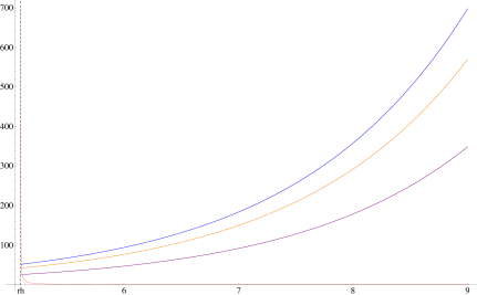
Figure 1: Horizon-shot and UV-shot solutions for metric functions at $s=1$, $c_{+}=3$, $C_{2}=800000$. $e^{k}$ - orange, $e^{g}$ - blue, $e^{h}$ - purple, $e^{8x}$ - pink

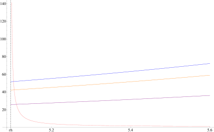
Figure 2: Horizon-shot and UV-shot solutions for metric functions at $s=1$, $c_{+}=3$, $C_{2}=800000$. Zoomed into region near horizon at $\rho_{h}\sim$ 5.097.

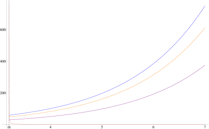
Figure 3: Horizon-shot and UV-shot solutions for metric functions at $s=1$, $c_{+}=50$, $C_{2}=5000$.

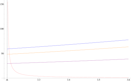
Figure 4: Horizon-shot and UV-shot solutions for metric functions at $s=1$, $c_{+}=50$, $C_{2}=5000$. Zoomed into region near horizon at $\rho_{h}\sim$ 3.19

3.4 Temperature of the solutions

The expression for the horizon temperature of our solutions follows from the standard prescription of analytically continuing the solution to Euclidean time and imposing the periodicity of this coordinate. The temperature is then given by $T=1/\beta$, where the period $\beta$ is determined by requiring the regularity of the Euclideanized metric at the horizon. We use the numerically determined parameters described in section 3.2 to describe the metric at the horizon; of these parameters, only $x_{1}$ and $k_{0}$ enter into the expression for the temperature, which is found to be

$$T_{hor}=\frac{1}{4\pi}\frac{x_{1}}{\sqrt{k_{0}}}.$$ (34)

In HEATING it was shown that the horizon temperature is the same for pre- and post-rotated solutions. It can be checked that this is still the case here.

In Figs.(6) and (6) we see that, for fixed values of $c_{+}$ and $C_{2}$, the horizon temperature has negligible dependence on $s\equiv N_{f}/N_{c}$. As we vary $0\leq s<\,\sim 10$ the temperature remains constant; we conclude that the temperature is not affected by the backreaction of the flavor branes.

In Figs.(8), (8) and (10) we show how the horizon temperature varies with $C_{2}$ for fixed values of $c_{+}$ and $s$. In Fig. (10) we present the temperature as a function of the horizon area. Note that as $C_{2}$ decreases the temperature increases indicating that it diverges in the extremal limit. Also, for $C_{2}\rightarrow\infty$ figure (10) shows that the temperature goes to a very small but non-zero value, $T_{c}$. This behavior is reminiscent of the wrapped five branes black holes of GTV . In that framework $T_{c}$ is the Hagedorn temperature of the little string theory and is also a critical temperature at which a first order phase transition occurs (chiral symmetry restoration and deconfinement) GTV . A similar phase transition could exist here. If that is the case, the U-dualities described in the following section will probably map it to a phase transition in Klebanov-Strassler. This is an issue that deserves further study.

Figure 5: Temperature at the horizon versus $N_{f}/N_{c}$. $c_{+}=50,C_{2}=5000$.

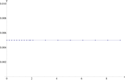
Figure 6: Temperature at the horizon versus $N_{f}/N_{c}$. $c_{+}=3,C_{2}=800000$.

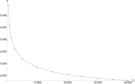
Figure 7: Temperature at the horizon versus $C_{2}$. $c_{+}=50,s=1$.

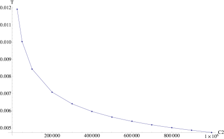
Figure 8: Temperature at the horizon versus $C_{2}$. $c_{+}=3,s=1$.

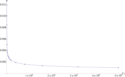
Figure 9: Temperature at the horizon versus for very large values of $C_{2}$. $c_{+}=3,s=1$.

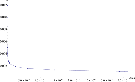
Figure 10: Temperature at the horizon versus $\mathcal{A}/V_{3}$. $c_{+}=3,s=1$.

4 Non-extremal backgrounds with flavored resolved deformed conifold asymptotics

In Maldacena:2009mw the authors presented a solution generating technique that takes a IIB background of $D5$ branes wrapped on the $S^{2}$ of the resolved conifold (non-trivial $F_{(3)}$ and $\phi$) and produces a background wich also has $D3$ charge (non trivial $F_{(3)},F_{(5)},H_{(3)}$ and $\phi$). After a scaling limit the resulting geometry represents the baryonic branch of the Klebanov-Strassler solution. The initial space has topology $R^{1,3}\times\mathcal{M}_{6}$ and preserves $\mathcal{N}=1$ supersymmetry . The algorithm consists of performing three T-dualities in the $R^{3}$ directions, lifting to M-theory, boosting with rapidity $\beta$ in the eleventh direction, reducing back to ten dimensions and finally T-dualizing back in $R^{3}$. This procedure is equivalent to a rotation in the space of Killing spinors. We will therefore refer to this algorithm indistinctively as a chain of dualities or as a rotation.

In the previous section we found non-extremal solutions representing a background of $N_{c}$ wrapped color $D5$ branes and $N_{f}$ smeared $D5$ flavor branes $(N_{f}/N_{c}\sim 1)$. In this section we want to apply the procedure developed in Maldacena:2009mw to these backgrounds.

After applying the rotation procedure, taking $\beta\to\infty$ to decouple the gravitational modes, and performing the rescalings as described in HEATING , we obtain the transformed solutions in Einstein frame (see Appendix D for details):

$$ds_{IIB}^{2}=N_{c}\Big{[}e^{-\phi/2}\mathcal{H}^{-1/2}(-e^{-8x}dt^{2}+dx_{i}dx^{i})+e^{3\phi/2}\mathcal{H}^{1/2}ds_{6}^{2}\Big{]},$$

$$F_{(3)}=\frac{N_{c}}{4}f_{(3)},\;\;\;H_{(3)}=-e^{-4x}\frac{N_{c}}{4}\,e^{2\phi}\,*_{6}f_{(3)},$$

$$F_{(5)}=-N_{c}^{2}(1+*_{10})\left[\mathrm{Vol_{(4)}}\wedge d\left(\frac{e^{-4x}}{\mathcal{H}}\right)\right],$$ (35)

where

$$\mathcal{H}^{1/2}=\sqrt{e^{-2\phi}-e^{-8x}}$$ (36)

and the explicit forms of $f_{(3)}$ and $ds_{6}^{2}$ are given in equations (LABEL:eq:F3ansatz) and (2.2) respectively. Note that, unlike more standard finite temperature solutions where the non-extremality factor $e^{-8x}$ enters only in the $g_{rr}$ and $g_{tt}$ elements of the metric, here the warp factor $\mathcal{H}$ and the fluxes $F_{(5)}$ and $H_{(3)}$ depend on $e^{-8x}$.

The use of U-dualities is a well stablished solution generating technique in supergravity. In the presence of smeared flavored branes one could question the validity and meaning of the uplift to eleven dimensions. Two pieces of knowledge provide useful insight on this issue:

1. In Gaillard:2009kz the authors studied the uplift of smeared $D6$ flavor branes to M-theory. They argued that the violation of the Bianchi identity in ten dimensions implies that the eleven dimensional-geometry will no longer be Ricci flat; it is no longer of $G_{2}$ holonomy but it does carry $G_{2}$ structure. Thus, the flavors appear in eleven dimensions as intrinsic torsion. This eleven dimensional theory is no longer maximally supersymmetric (it is $1/8$ BPS) and therefore it is no longer unique. This is an interesting possibility for the interpretation of the uplift of smeared flavor branes. For us, however, the important point is that once the reduction to ten dimensions is carried out the correct smearing form is recovered.

2. In WARPED the authors studied a transformation to generate $SU(3)$ structure solutions of IIB supergravity starting from non-Kähler backgrounds describing wrapped $D5$ branes with additional flavor (smeared) $D5$ branes. Working with the BPS equations and the $SU(3)$ structure of the backgrounds they presented a solution generating technique that amounts to a rotation in the space of Killing spinors. This rotation procedure is well defined (even in the presence of smeared flavor branes) and is equivalent to the chain of U-dualities alluded to above.

In the present work we are dealing with a non-extremal deformation of WARPED . However, since the backgrounds we are working with are not supersymmetric, we cannot use the BPS formalism of WARPED . On the other hand, we are not interested in the interpretation of the background in eleven dimensions, so we will not attempt to address the questions presented in Gaillard:2009kz . Instead, guided by the results of WARPED , we will forge ahead and apply the chain of dualities to the flavored, non extremal backgrounds with stabilized dilaton found in section 3. However in order to claim that the outcome of these dualities is still a solution of IIB plus sources, we have to show that the rotated backgrounds are indeed a solution of the EOMs.

4.1 Equations of motion with $D3$ and $D5$ charges and smeared flavor branes

In this section we will verify that given the EOMs before the rotation procedure is applied, the EOMs after the rotation are also satisfied. The EOMs before rotation were presented in section 2.2 and derived in Appendix A. After the rotation procedure is carried out, the supergravity background contains $H_{(3)}$ and $F_{(5)}$ fluxes in addition to the $F_{(3)}$ that was present before rotation. The full type IIB action, supplemented by the DBI action for the smeared flavor branes, is then given by

$$S=S_{IIB}+S_{\text{sources}}$$ (37)

where

$$S_{IIB}=\frac{1}{2\kappa_{10}^{2}}\int \sqrt{-g}R-\frac{1}{4\kappa_{10}^{2}}\int\left(\vphantom{\frac{1}{2}}d\phi\wedge*d\phi+e^{-\phi}H_{(3)}\wedge*H_{(3)}\right.$$

$$+\left.e^{\phi}F_{(3)}\wedge*F_{(3)}+\frac{1}{2}F_{(5)}\wedge*F_{(5)}-C_{(4)}\wedge F_{(3)}\wedge H_{(3)}\right),$$ (38)

and

$$S_{\text{sources}}=-\frac{4T_{5}}{(4\pi)^{2}}\int \left(\mathrm{Vol_{(4)}}\wedge d\rho\wedge d\psi\;e^{\phi/2}\sqrt{|g_{ab}+e^{-\phi/2}B_{ab}|}\right.$$

$$-\left.\vphantom{\sqrt{|e({-B}|}}C_{(6)}+C_{(4)}\wedge B_{(2)}\right)\wedge\Xi_{(4)}$$

Note that the metric is in Einstein frame and that $g_{ab}$ and $B_{ab}$ respectively represent the pullbacks of the metric and $B_{(2)}$ to the flavor brane world volume. Recall that before rotation $H_{(3)}=0$ and thus, the DBI action was only the pullback of the metric. After rotation we need to specify the form of the NS potential, $B_{(2)}$. In the extremal case ($T=0$), this potential should reduce to the one in WARPED . We propose the following ansätz:

$$B_{(2)}=b_{1}(\rho)\tilde{\omega_{3}}\wedge d\rho+b_{2}(\rho)e_{1}\wedge e_{2}+b_{3}e_{1}\wedge\tilde{\omega}_{2}+b_{4}(\rho)e_{2}\wedge\tilde{\omega}_{1}+b_{5}(\rho)\tilde{\omega}_{1}\wedge\tilde{\omega}_{2}.$$ (40)

To make the gauge degrees of freedom more apparent it is convenient to parameterize $B_{(2)}$ in a slightly different way. Let us introduce $b_{2}(\rho)=\widetilde{b_{2}}(\rho)+(1-a(\rho)^{2})b_{5}(\rho)$. It is then easy to verify that

$$B_{(2)}=B_{(2)}|_{b_{5}=0}-d\left[b_{5}(\rho)\tilde{\omega_{3}}\right]$$ (41)

with $b_{5}(\rho)$ an undetermined function. It is clear that any $b_{5}(\rho)$ results in the same $H_{(3)}$, and that $b_{5}$ is just a gauge degree of freedom. Demanding that $H_{(3)}=d[B_{(2)}]$, we get 5 equations. This system of equations can be reduced to just one differential equation. We choose a gauge such that $b_{1}(\rho)$ coincides with the one in WARPED (see Appendix E for details).

The flavor brane world volume is $dt\wedge dx_{1}\wedge dx_{2}\wedge dx_{3}\wedge d\rho\wedge d\psi\equiv\mathrm{Vol_{(4)}}\wedge d\rho\wedge d\psi$, and the smearing form is given by $\Xi_{(4)}=\frac{s}{4}\sin\theta\sin\tilde{\theta}\,d\theta\wedge d\varphi\wedge d\tilde{\theta}\wedge d\tilde{\varphi}$, where we have set $\alpha^{\prime}=g_{s}=1$. As was the case before rotation, the $C_{(6)}\wedge\Xi_{(4)}$ term in the source action vanishes. Note that in the EOMs that follow from this action, the contribution from the Wess-Zumino term in the source action is exactly cancelled by that from the Chern-Simons term in the bulk.

The Bianchi identities for the RR and NS-NS forms after rotation are

$$dF_{(3)}=\Xi_{(4)},\qquad dH_{(3)}=0,\qquad dF_{(5)}+F_{(3)}\wedge H_{(3)}=B_{(2)}\wedge\Xi_{(4)}$$ (42)

The first is unchanged from before the rotation, and the latter two can be checked to hold given the EOMs before rotation. Note that this does not give us the full expression for $B_{(2)}$, but only the components which are orthogonal to $\Xi_{(4)}$, namely $B_{\rho\psi}$. However $B_{(2)}$ only appears in the source action, and there it is either wedged with $\Xi_{(4)}$, or pulled back to the flavorbrane world volume (which is orthogonal to $\Xi_{(4)}$). Therefore only this orthogonal component will be relevant for our equations of motion. A more detailed derivation of the general form of $B_{(2)}$ is given in Appendix E.

The EOMs for the fluxes after rotation are

$$d\left(e^{-\phi}*H_{(3)}\right)=F_{(3)}\wedge F_{(5)}+\frac{e^{-8x}}{\mathcal{H}}\;\mathrm{Vol_{(4)}}\wedge\Xi_{(4)}$$ (43)

$$d\left(e^{\phi}*F_{(3)}\right)=-H_{(3)}\wedge F_{(5)}$$ (44)

where the term with $\mathcal{H}$ in the first equation comes from varying the source term. These can be checked to hold given the EOMs before rotation.

The dilaton EOM is

$$d\left(*d\phi\right) = \frac{e^{\phi}}{2}F_{(3)}\wedge*F_{(3)}-\frac{e^{-\phi}}{2}H_{(3)}\wedge*H_{(3)}+\left(2\kappa_{10}^{2}\right)\frac{\delta\mathcal{L}_{\text{sources}}}{\delta\phi}$$

where

$$\frac{\delta\mathcal{L}_{\text{sources}}}{\delta\phi} =\frac{1}{2}e^{\phi/2}\left(\sqrt{|g_{ab}+e^{-\phi/2}B_{ab}|}-\frac{|g_{(4)}|e^{-\phi}B_{\rho\psi}^{2}}{\sqrt{|g_{ab}+e^{-\phi/2}B_{ab}|}}\right)\ \mathrm{Vol_{(4)}}\wedge d\rho\wedge d\psi\wedge\Xi_{(4)}$$ (45)

and can be checked to hold given the EOMs before rotation.

Lastly, we have the Einstein equations

$$R_{\mu\nu}-\frac{1}{2}g_{\mu\nu}R=\ \frac{1}{2}\left(\partial_{\mu}\phi\partial_{\nu}\phi-\frac{1}{2}g_{\mu\nu}\partial_{\lambda}\phi\partial^{\lambda}\phi\right)+\frac{1}{12}e^{\phi}\left(3F_{\mu\alpha\beta}F_{\nu}^{\alpha\beta}-\frac{1}{2}g_{\mu\nu}F_{(3)}^{2}\right)$$

$$+\frac{1}{12}e^{-\phi}\left(3H_{\mu\alpha\beta}H_{\nu}^{\alpha\beta}-\frac{1}{2}g_{\mu\nu}H_{(3)}^{2}\right)+\frac{1}{96}\left(F_{\mu\alpha\beta\gamma\delta}F_{\nu}^{\alpha\beta\gamma\delta}\right)+T^{\,\text{sources}}_{\mu\nu}$$ (46)

where the variation of the Chern-Simons term in the bulk action is cancelled by the variation of the Wess-Zumino term in the source action. Here, $T^{\,\text{sources}}_{\mu\nu}$ is obtained from (after rotation)

$$T^{\mu\nu}_{\text{sources}} = \frac{2\kappa_{10}^{2}}{\sqrt{-g_{(10)}}}\frac{\delta\mathcal{L}_{\text{sources}}}{\delta g_{\mu\nu}},$$ (47)

and has components:

$$T^{\,\text{sources}}_{tt}=\frac{s\,e^{-2g-2h-8x-4\phi}}{2\mathcal{H}^{2}}\,\,,\qquad\qquad T^{\,\text{sources}}_{x_{i}x_{j}}=-\frac{s\,\eta_{ij}e^{-2g-2h-4\phi}}{2\mathcal{H}^{2}}\,,$$

$$T^{\,\text{sources}}_{\rho\rho}=-\frac{s}{2}e^{-2g-2h+2k+8x},\qquad\qquad T^{\,\text{sources}}_{\psi\psi}=-\frac{s}{8}e^{-2g-2h+2k}\,\,,$$

$$T^{\,\text{sources}}_{\varphi\psi}=-\frac{s}{8}e^{-2g-2h+2k}\cos\theta\,\,,\qquad\qquad T^{\,\text{sources}}_{\varphi\varphi}=-\frac{s}{8}e^{-2g-2h+2k}\cos^{2}\theta\,\,,$$

$$T^{\,\text{sources}}_{\tilde{\varphi}\psi}=-\frac{s}{8}e^{-2h-2g+2k}\cos\tilde{\theta}\,\,,\qquad\qquad T^{\,\text{sources}}_{\tilde{\varphi}\tilde{\varphi}}=-\frac{s}{8}e^{-2h-2g+2k}\cos^{2}\tilde{\theta}\,\,,$$

$$T^{\,\text{sources}}_{\varphi\tilde{\varphi}}=-\frac{s}{8}e^{-2h-2g+2k}\cos\theta\cos\tilde{\theta}\,.$$

Again, the Einstein equations can be checked to hold given the EOMs before rotation.

4.2 Rotating the solutions

It is now a simple procedure to use equations (35) along with our numerical solutions to produce numerical solutions for the background after rotation. Before presenting and commenting on the numerical results let look at the large $\rho$ behavior.

4.2.1 Asymptotics after the rotation

In order to write down the form of the metric the UV after the rotation, we identify from (35),

$$g_{xx}=e^{-\phi/2}\mathcal{H}^{-1/2}\qquad g_{tt}=e^{-\phi/2-8x}\mathcal{H}^{-1/2}\qquad g_{\rho\rho}=e^{3\phi/2}\mathcal{H}^{1/2}e^{2k+8x}$$

$$g_{\theta\theta}=e^{3\phi/2}\mathcal{H}^{1/2}e^{2h}\qquad g_{\tilde{\theta}\tilde{\theta}}=e^{3\phi/2}\mathcal{H}^{1/2}\frac{e^{2g}}{4}\qquad g_{\psi\psi}=e^{3\phi/2}\mathcal{H}^{1/2}\frac{e^{2k}}{4}$$

Using (3.1) and (LABEL:eq:identify-metric-after) we obtain,

$$g_{xx}\sim\frac{\sqrt{\frac{2c_{+}}{3}}e^{2\rho/3}}{\sqrt{s}}-\frac{e^{-2\rho/3}}{24\sqrt{6c_{+}}s^{3/2}}\bigg{(}16c_{+}^{2}C_{2}+3\left(-2+s(2-16\rho)+16\rho+s^{2}(1+4\rho)\right)\bigg{)}+\cdots$$

$$-g_{tt}\sim\frac{\sqrt{\frac{2c_{+}}{3}}e^{2\rho/3}}{\sqrt{s}}-\frac{e^{-2\rho/3}}{24\sqrt{6c_{+}}s^{3/2}}\bigg{(}16c_{+}^{2}C_{2}+3\left(-2+s(2-16\rho)+16\rho+s^{2}(1+4\rho)\right)\bigg{)}+\cdots$$

$$g_{\rho\rho}\sim\sqrt{\frac{2c_{+}}{3}}e^{2\rho/3}\sqrt{s}+\frac{e^{-2\rho/3}}{24\sqrt{6c_{+}}\sqrt{s}}\bigg{(}-6+16c_{+}^{2}C_{2}+s(6-48\rho)+48\rho+3s^{2}(-11+4\rho)\bigg{)}+\cdots$$

$$g_{\theta\theta}\sim\sqrt{\frac{3c_{+}}{2}}e^{2\rho/3}\sqrt{s}+\frac{e^{-2\rho/3}}{64\sqrt{6c_{+}}\sqrt{s}}\bigg{(}-6+16c_{+}^{2}C_{2}+s^{2}(9-36\rho)+48\rho+6s(-7+8\rho)\bigg{)}+\cdots$$

$$g_{\tilde{\theta}\tilde{\theta}}\sim\sqrt{\frac{3c_{+}}{2}}e^{2\rho/3}\sqrt{s}+\frac{e^{-2\rho/3}}{64\sqrt{6c_{+}}\sqrt{s}}\bigg{(}-6+16c_{+}^{2}C_{2}+48\rho-18s(-3+8\rho)+s^{2}(-39+60\rho)\bigg{)}+\cdots$$

$$g_{\psi\psi}\sim\frac{\sqrt{c_{+}}e^{2\rho/3}\sqrt{s}}{2\sqrt{6}}+\frac{e^{-2\rho/3}}{96\sqrt{6c_{+}}\sqrt{s}}\bigg{(}-6+16c_{+}^{2}C_{2}+s(6-48\rho)+48\rho+3s^{2}(-11+4\rho)\bigg{)}+\cdots\\$$ (50)

It is clear that this expansion is not valid as $s\rightarrow 0$. However, this does not mean that we cannot obtain the expected KS asymptotics in that limit. It just indicates that we should take the $s\rightarrow 0$ limit before performing the rotation. Indeed, setting $s=0$ before the rotation in (3.1) and defining $c_{+}\sqrt{8}A(\rho)=\sqrt{24\rho+8C_{2}c_{+}^{2}-3}$ to avoid clutter we obtain the following metric after rotation ,

$$g_{xx}\sim\frac{e^{4\rho/3}}{A(\rho)}+\frac{e^{-4\rho/3}}{2048c_{+}^{4}A(\rho)^{3}}\bigg{(} 16c_{+}^{2}C_{2}\left(185-272\rho+128\rho^{2}\right)$$

$$+3\left(-847+3504\rho-3456\rho^{2}+2048\rho^{3}\right)\bigg{)}+\mathcal{O}(e^{-8\rho/3})$$

$$-g_{tt}\sim\frac{e^{4\rho/3}}{A(\rho)}+\frac{e^{-4\rho/3}}{2048c_{+}^{4}A(\rho)^{3}}\bigg{(} -2048c_{+}^{4}C_{2}^{2}+16c_{+}^{2}C_{2}\left(233-656\rho+128\rho^{2}\right)$$

$$+3\left(-847+3504\rho-3456\rho^{2}+2048\rho^{3}\right)\bigg{)}+\mathcal{O}(e^{-8\rho/3})$$

$$g_{\rho\rho}\sim\frac{2c_{+}}{3}A(\rho)+\mathcal{O}(e^{-8\rho/3})\quad\quad g_{\theta\theta}\sim\frac{c_{+}}{4}A(\rho)+\frac{e^{-4\rho/3}}{4}A(\rho)(2\rho-1)+\mathcal{O}(e^{-8\rho/3})$$

$$g_{\psi\psi}\sim\frac{1}{6}c_{+}A(\rho)+\mathcal{O}(e^{-8\rho/3})\quad\quad g_{\tilde{\theta}\tilde{\theta}}\sim\frac{c_{+}}{4}A(\rho)-\frac{e^{-4\rho/3}}{4}A(\rho)(2\rho-1)+\mathcal{O}(e^{-8\rho/3}).$$

Using a variable $u=e^{2\rho/3}$, the metric reads at leading order

$$ds^{2}=\frac{u^{2}}{A(u)}(dx_{i}dx^{i})+\frac{3cA(u)}{2}(\frac{du^{2}}{u^{2}}+ds^{2}_{T^{11}})+\cdots\mathcal{O}(u^{-2}),$$ (52)

where $A(u)=\frac{3}{c_{+}\sqrt{2}}\sqrt{\log u+\frac{2}{9}C_{2}c_{+}^{2}-\frac{1}{12}}$ contains the typical $\log$ behavior of KS asymptotics. . Note that, since numerically the work of finding non-extremal solutions is done before the rotation it is trivial for us to set $s$ to any value, however small, and then rotate.

4.2.2 Rotated flavored solutions

After rotating the numerical solutions obtained in Section 3 we obtain Figs.(12 – 18). Note that,

• The addition of flavor alters the behavior of the dilaton and the $g_{xx},g_{tt},g_{\rho\rho}$ parts of the metric in the UV, but not in the IR. On the other hand, flavor affects the metric of the compact manifold at all energy scales, as shown in Figs.(17, 18).

• Comparing $g_{\theta\theta}$ and $g_{\tilde{\theta}\tilde{\theta}}$ for $s=61/10$ and $s=2/5$ in Figs.(17, 18) we can see that the behavior of the curves has been swaped. For $s=61/10$, $g_{\tilde{\theta}\tilde{\theta}}$ grows as we approach the horizon while $g_{\theta\theta}$ decreases. For $s=2/5$ it is the other way around. This swapping occurs as we cross $s=2$.

• From (35) we can see that after the rotation the compact part of the metric is still an expanding $T^{1,1}$. This is also shown in(17, 18) where we can see that for large $\rho$ we have $g_{\theta\theta}\sim g_{\tilde{\theta}\tilde{\theta}}\sim\frac{3}{2}g_{\psi\psi}$.

Figure 11: $g_{\rho\rho}$ metric element for solutions after rotation, $c_{+}=50,\ C_{2}=5000$. From bottom to top: $s=0,1,19/10,51/10,91/10$.

Figure 12: $g_{\rho\rho}$ metric element for solutions after rotation, $c_{+}=3,\ C_{2}=800000$. From bottom to top: $s=0,1,19/10,51/10,91/10$.

Figure 13: $g_{xx}$ (red) and $g_{tt}$ (blue) metric elements for the unflavored solution after rotation: $c_{+}=50,\ C_{2}=5000,s=0$.

Figure 14: $g_{xx}$ (red) and $g_{tt}$ (blue) metric elements for the unflavored solution after rotation: $c_{+}=3,\ C_{2}=800000,s=0$.

Figure 15: $g_{xx}$ (red) and $g_{tt}$ (blue) metric elements for flavored solutions after rotation: $c_{+}=50,\ C_{2}=5000$. From top to bottom: $s=0,1,19/10,51/10,91/10$.

Figure 16: $g_{xx}$ (red) and $g_{tt}$ (blue) metric elements for flavored solutions after rotation: $c_{+}=3,\ C_{2}=800000$. From top to bottom: $s=0,1,19/10,51/10,91/10$.

Figure 17: $\frac{3}{2}g_{\psi\psi}$ (blue), $g_{\theta\theta}$ (red), and $g_{\tilde{\theta}\tilde{\theta}}$ (yellow) metric elements for flavored solution after rotation. The different groups correspond toi $s=0$ (solid), $s=2/5$ (dotted) and $s=61/10$ (dashed). $c_{+}=3$,  $C_{2}=800000$.

Figure 18: $\frac{3}{2}g_{\psi\psi}$ (blue), $g_{\theta\theta}$ (red), and $g_{\tilde{\theta}\tilde{\theta}}$ (yellow) metric elements for flavored solution after rotation. The different groups correspond to $s=0$ (solid), $s=2/5$ (dotted) and $s=61/10$ (dashed). $c_{+}=50$,  $C_{2}=50000$.

5 Energy and specific heat

In order to assess the thermodynamic stability of our solutions, we need to determine the specific heat, $C_{v}$. This is obtained from the expression for the ADM energy of our solutions and their temperature via the standard thermodynamic relation $C_{v}=\partial E/\partial T$. $T$ is the numerically determined temperature given in equation (34), and $E$ is given by the expression for the conserved ADM energy HAWKINGHOROWITZ (where $16\pi G_{10}=2\kappa_{10}^{2}=(2\pi)^{7}$)

$$E_{ADM}=-\frac{1}{8\pi G_{10}}\int_{S_{t}^{\infty}}\sqrt{|g_{00}|}(^{8}K-^{8}K_{0})dS_{t}^{\infty}.$$ (53)

Here, ${}^{8}K$ and ${}^{8}K_{0}$ are the extrinsic curvatures of two 8-dimensional submanifolds $S_{t}$ of $\Sigma_{t}$ at constant $\rho$. $\Sigma_{t}$ is a constant-time 9d spatial slice of the entire geometry, and we take for $S_{t}$ the boundary manifold $S_{t}^{\infty}$ as $\rho\to\infty$. ${}^{8}K$ corresponds to our finite temperature backgrounds, whereas ${}^{8}K_{0}$ is the extrinsic curvature of a reference background HAWKINGHOROWITZ ; Cotrone:2007qa . For the reference background, we take one of the family of zero-temperature BPS solutions discussed in WARPED ; HoyosBadajoz:2008fw . The UV asymptotics of these backgrounds are summarized in Appendix B.2.

Our Euclideanized 10d metric reads

$$ds^{2}=g_{00}d\tau^{2}+g_{xx}dx_{i}dx^{i}+g_{\rho\rho}d\rho^{2}+g_{\theta\theta}(e_{1}^{2}+e_{2}^{2})+g_{\tilde{\theta}\tilde{\theta}}(\tilde{\omega}_{1}^{2}+\tilde{\omega}_{2}^{2})+g_{\psi\psi}\,\tilde{\omega}_{3}^{2}.$$ (54)

The metric on a constant time slice $\Sigma_{t}$, and on its 8-dimensional boundary $S_{t}^{\infty}$ are

$$ds^{2}_{\Sigma_{t}}=g_{xx}dx_{i}dx^{i}+g_{\rho\rho}d\rho^{2}+g_{\theta\theta}(e_{1}^{2}+e_{2}^{2})+g_{\tilde{\theta}\tilde{\theta}}(\tilde{\omega}_{1}^{2}+\tilde{\omega}_{2}^{2})+g_{\psi\psi}\,\tilde{\omega}_{3}^{2}$$ (55)

$$ds^{2}_{S_{t}^{\infty}}=g_{xx}dx_{i}dx^{i}+g_{\theta\theta}(e_{1}^{2}+e_{2}^{2})+g_{\tilde{\theta}\tilde{\theta}}(\tilde{\omega}_{1}^{2}+\tilde{\omega}_{2}^{2})+g_{\psi\psi}\,\tilde{\omega}_{3}^{2},$$ (56)

where the metric functions in Einstein frame are

$$g_{00} =e^{\phi/2}e^{-8x}\quad\quad\quad\quad g_{00_{B}} =e^{\phi_{B}/2}\nu_{B}$$

$$g_{xx} =e^{\phi/2} g_{xx_{B}} =e^{\phi_{B}/2}$$

$$g_{\rho\rho} =e^{\phi/2}e^{8x}e^{2k} g_{\rho\rho_{B}} =e^{\phi_{B}/2}e^{2k_{B}}$$

$$g_{\theta\theta} =e^{\phi/2}e^{2h} g_{\theta\theta_{B}} =e^{\phi_{B}/2}e^{2h_{B}}$$

$$g_{\tilde{\theta}\tilde{\theta}} =\frac{1}{4}e^{\phi/2}e^{2g} g_{\tilde{\theta}\tilde{\theta}_{B}} =\frac{1}{4}e^{\phi_{B}/2}e^{2g_{B}}$$

$$g_{\psi\psi} =\frac{1}{4}e^{\phi/2}e^{2k} g_{\psi\psi_{B}} =\frac{1}{4}e^{\phi_{B}/2}e^{2k_{B}}$$

before rotation, and

$$g_{00} =e^{-\phi/2}\mathcal{H}^{-1/2}e^{-8x}\quad\quad\quad\quad g_{00_{B}} =e^{-\phi_{B}/2}\mathcal{H}_{B}^{-1/2}\nu_{B}$$

$$g_{xx} =e^{-\phi/2}\mathcal{H}^{-1/2} g_{xx_{B}} =e^{-\phi_{B}/2}\mathcal{H}_{B}^{-1/2}$$

$$g_{\rho\rho} =e^{3\phi/2}\mathcal{H}^{1/2}e^{8x}e^{2k} g_{\rho\rho_{B}} =e^{3\phi_{B}/2}\mathcal{H}_{B}^{1/2}\,e^{2k_{B}}$$

$$g_{\theta\theta} =e^{3\phi/2}\mathcal{H}^{1/2}e^{2h} g_{\theta\theta_{B}} =e^{3\phi_{B}/2}\mathcal{H}_{B}^{1/2}e^{2h_{B}}$$

$$g_{\tilde{\theta}\tilde{\theta}} =\frac{1}{4}e^{3\phi/2}\mathcal{H}^{1/2}e^{2g} g_{\tilde{\theta}\tilde{\theta}_{B}} =\frac{1}{4}e^{3\phi_{B}/2}\mathcal{H}_{B}^{1/2}e^{2g_{B}}$$

$$g_{\psi\psi} =\frac{1}{4}e^{3\phi/2}\mathcal{H}^{1/2}e^{2k} g_{\psi\psi_{B}} =\frac{1}{4}e^{3\phi_{B}/2}\mathcal{H}_{B}^{1/2}e^{2k_{B}}$$

after rotation; ‘$B$’ subscripts indicate the BPS backgrounds. Here $\mathcal{H}=(e^{-2\phi}-e^{-8x})$ and $\mathcal{H}_{B}=(e^{-2\phi_{B}}-\kappa_{2}^{2})$, where $\kappa_{2}$ is a free parameter with $0<\kappa_{2}<e^{-\phi_{\infty}}$ that parametrizes the rotation, see WARPED . In terms of the 11d boost parameter $\beta$, we have $\kappa_{2}=e^{-\phi_{\infty}}\tanh{\beta}$. Note that for the BPS solutions $e^{-8x}=1$, and we have also allowed for an arbitrary rescaling of the $\tau$ coordinate via a constant parameter $\nu_{B}$, reflecting the freedom in choosing the period $\beta$ of the Euclidean time coordinate for these backgrounds.

It is now straightforward to calculate the extrinsic curvature of an 8-manifold $S_{t}$ at constant $\rho$. We obtain

$$^{8}K_{bef}=e^{-\frac{\phi(\rho)}{4}-k(\rho)-4x(\rho)}\left(2\phi^{\prime}(\rho)+2g^{\prime}(\rho)+2h^{\prime}(\rho)+k^{\prime}(\rho)\right)$$ (59)

for the background before rotation, and

$$^{8}K_{aft} =\frac{1}{2}\frac{\mathcal{H}(\rho)}{\mathcal{H}(\rho)^{5/4}}e^{-\frac{3\phi(\rho)}{4}-k(\rho)-4x(\rho)}$$

$$+\frac{1}{\mathcal{H}(\rho)^{1/4}}e^{-\frac{3\phi(\rho)}{4}-k(\rho)-4x(\rho)}\bigg{(}3\phi^{\prime}(\rho)+2g^{\prime}(\rho)+2h^{\prime}(\rho)+k^{\prime}(\rho)\bigg{)}$$ (60)

for the rotated background.

The expressions for $dS_{t}$ are

$$dS_{t_{bef}}=\frac{1}{8}e^{2\phi}e^{2g+2h+k}dV_{3}\wedge dS_{\mathcal{M}_{6}}\quad\quad\quad dS_{t_{aft}}=\frac{1}{8}\mathcal{H}^{1/2}e^{3\phi}e^{2g+2h+k}dV_{3}\wedge dS_{\mathcal{M}_{6}}$$ (61)

where $dV_{3}=dx_{1}\wedge dx_{2}\wedge dx_{3}$ is the volume form on the Minkowski spatial directions, and $dS_{\mathcal{M}_{6}}=(\sin\theta\sin\tilde{\theta})d\theta\wedge d\varphi\wedge d\tilde{\theta}\wedge d\tilde{\varphi}\wedge d\psi$ is the volume form on the compact cycles. Putting all of these together and integrating over the compact $\theta,\varphi,\tilde{\theta},\tilde{\varphi},\psi$ directions we obtain expressions for the ADM energy before and after the rotation:

$$e_{bef}=\frac{E_{bef}}{V_{3}}=-\frac{1}{8\pi^{4}}\bigg{[} e^{-8x}e^{2\phi+2g+2h}\bigg{(}2(\phi^{\prime}+g^{\prime}+h^{\prime})+k^{\prime}\bigg{)}$$

$$-\sqrt{\nu_{B}}\,e^{2\phi_{B}+2g_{B}+2h_{B}}\bigg{(}2(\phi_{B}^{\prime}+g_{B}^{\prime}+h_{B}^{\prime})+k_{B}^{\prime}\bigg{)}\bigg{]}\Bigg{|}_{\rho\to\infty}$$ (62)

$$e_{aft}=-\frac{1}{8\pi^{4}}\bigg{[} e^{-8x}e^{2\phi+2g+2h}\bigg{(}\frac{\mathcal{H}^{\prime}}{2\mathcal{H}}+\big{(}3\phi^{\prime}+2(g^{\prime}+h^{\prime})+k^{\prime}\big{)}\bigg{)}$$

$$-\sqrt{\nu_{B}}\,e^{2\phi_{\small{B}}+2g_{B}+2h_{B}}\bigg{(}\frac{\mathcal{H}^{\prime}_{B}}{2\mathcal{H}_{B}}+\big{(}3\phi_{B}^{\prime}+2(g_{B}^{\prime}+h_{B}^{\prime})+k_{B}^{\prime}\big{)}\bigg{)}\bigg{]}\Bigg{|}_{\rho\to\infty}$$ (63)

Here $V_{3}$ = Vol($R^{3}$), and we have expressed the results as energy densities per unit flat 3-volume.

We evaluate these expressions at a large but finite value of $\rho=\rho_{*}$ by inserting the UV asymptotics of the BPS and finite temperature solutions. The BPS asymptotics are given in terms of the free variables $Q_{o},c_{+},c_{-},\rho_{0}$ and $f_{1,0}$, and are listed in Appendix B.2. The finite temperature asymptotics were given in section 3.1, and are a deformation of a BPS background with $Q_{o}=-N_{c}+N_{f}/2$ and $\rho_{0}=0$.

In order to calculate the ADM energy, we first match the geometries and matter fields of the BPS and finite temperature backgrounds at $\rho_{*}$, this amounts to matching the metric functions $g_{00},g_{xx},g_{\theta\theta},g_{\tilde{\theta}\tilde{\theta}},g_{\psi\psi}$, as well as the dilaton. Only after this matching is performed we let $\rho_{*}\to\infty$.

We begin with the case before rotation. To avoid confusion with the parameters $c_{+}$ and $c_{-}$ in the finite temperature solutions, we will write the BPS $c_{+}$ and $c_{-}$ parameters in bold as $\mathbb{c_{+}}$ and $\mathbb{c_{-}}$. First we pick some fixed values of $c_{+},C_{2}$ and $s$ to specify the finite temperature background. We begin the matching by using the freedom in $\nu_{B}$ to set $\nu_{B}=e^{-8x(\rho_{*})}$. Next we match $e^{\phi/2}=e^{\phi_{B}/2}$ to $\mathcal{O}(e^{-12\rho_{*}/3})$ by setting

$$f_{1,0}=1-e^{-12\rho_{*}/3}\frac{C_{2}s}{c_{+}}.$$ (64)

As a result, $g_{00}$ and $g_{xx}$ are now matched to $\mathcal{O}(e^{-12\rho_{*}/3})$. Now, we match $e^{2k}=e^{2k_{B}},e^{2h}=e^{2h_{B}},$ and $e^{2g}=e^{2g_{B}},$ respectively, to $\mathcal{O}(e^{-8\rho_{*}/3})$, by setting

$$\mathbb{c_{+}} =c_{+}+e^{-12\rho_{*}/3}\frac{11C_{2}s}{48}$$

$$Q_{0} =-1+\frac{s}{2}-\frac{1}{16}e^{-8\rho_{*}/3}C_{2}(-5+4\rho_{*})(-2+s)$$

$$\mathbb{c_{-}} =\frac{2}{3}c_{+}^{2}(-11C_{2}s+4C_{2}s\rho_{*}),$$ (65)

which results in the matching of $g_{\theta\theta},g_{\tilde{\theta}\tilde{\theta}},g_{\psi\psi}$ to $\mathcal{O}(e^{-8\rho_{*}/3})$.

With these definitions, the dilaton and all of the metric functions $g_{00},g_{xx},g_{\theta\theta},g_{\tilde{\theta}\tilde{\theta}},g_{\psi\psi}$ are matched up to (at least) $\mathcal{O}(e^{-8\rho_{*}/3})$. The freedom in the $\rho_{0}$ parameter in the BPS solutions is not needed, and we set it equal to zero as was done for the finite temperature solutions. Taking $\rho_{*}\to\infty$, the resulting ADM energy density is finite, independent of $s$, and equal to

$$e_{bef}=\frac{5c_{+}^{2}C_{2}}{96\pi^{4}}$$ (66)

After the rotation, the presence of $\mathcal{H}$ causes the mixing of the UV asymptotics in the metric functions to become slightly more involved. The rotation also causes the metric function expansions to become unwieldy at higher order, so we only perform the matching to $\mathcal{O}(e^{-2\rho_{*}})$ which is enough to render the ADM energy finite. Despite these technical complications the process proceeds as above. Namely, before taking the $\rho_{*}\rightarrow\infty$ limit we fix coefficients so that the BPS and finite temperature metrics match at the boundary, we then take the $\rho_{*}\rightarrow\infty$ limit and obtain a finite energy given by

$$e_{aft}=\frac{5c_{+}^{2}C_{2}}{96\pi^{4}}.$$ (67)

Thus, the energy remains the same as before the rotation.

The above analysis was done for flavored finite-temperature backgrounds with $s\neq 0$. However, since the results do not depend on $s$ they should also hold for backgrounds without flavor i.e for non-extremal deformations that, after the rotation, do have Klebanov-Strassler asymptotics. We have explicitly checked that this is indeed the case.

In Fig. (19) we plot $de/d\mathfrak{s}$ and $T$ as functions of the entropy density (or equivalently the “radius” of the horizon) for solutions before the rotation. The overlap of the two curves show that the numerical solutions satisfy the first law of thermodynamics

$$de=Td\mathfrak{s}.$$ (68)

To verify that this is also the case after the rotation recall that we have already shown that the temperature and energy density remain the same (66),(67),(34). It is easy to see that the entropy density is also unaffected by the rotation,

$$\mathfrak{s}_{bef}=\frac{S_{\text{bef}}}{V_{3}}=\left.\frac{e^{2\phi}e^{2h+2g+k}}{4\pi^{3}}\right|_{\rho=\rho_{h}}$$ (69)

$$\mathfrak{s}_{aft}=\frac{S_{\text{aft}}}{V_{3}}=\left.\frac{e^{3\phi}\mathcal{H}^{1/2}e^{2h+2g+k}}{4\pi^{3}}\right|_{\rho=\rho_{h}}=\left.\frac{e^{3\phi}(e^{-2\phi}-e^{-8x})^{1/2}e^{2h+2g+k}}{4\pi^{3}}\right|_{\rho=\rho_{h}}=\mathfrak{s}_{\text{bef}}$$ (70)

where the last equality in equation (70) follows from the fact that $e^{-8x}$ vanishes at the horizon.

Thus, the thermodynamical quantities $e,\mathfrak{s}$ and $T$ are not modified by the rotation and the first law will still hold.

Figure 19: $de_{bef}/d\mathfrak{s}_{bef}$ ( red line) and $T_{h}$ ( blue dots) plotted vs. $\mathfrak{s}_{bef}$, for the flavored case with $c_{+}=50$, $s=1$.

As discussed in section 3.4, our numerics associate a horizon temperature with a choice of $c_{+}$ and $C_{2}$. In Figs.(21) and (21) we plot the energy density versus the associated temperature for a solution with $s=1$. The slope of these plots is the specific heat $C_{v}$ and is seen to be negative both before and after the rotation. Note that the fact that the first law is satisfied implies that we would have gotten the same answer had we chosen to use holographic renormalization methods.

The backreaction of the flavor branes does not play any role in the stability analysis as the temperature’s dependence on $s$ is essentially negligible compared to its dependence on $C_{2}$ and neither the energy nor the entropy depend on $s$. In Figs.(23) and (23) we show the energy density versus the entropy density $S/V_{3}$. Note that in Figs.(23) and (23) the behavior of the energy vs. entropy is linear for large values of $S$ (or equivalently for large values of the horizon “radius”). From the first law of thermodynamics, $dE=TdS$, we expect this to happen when the temperature is constant.

Thus, we have shown that, despite of having very different asymptotics, the backgrounds after the rotation have thermodynamical properties similar to the $D5$ wrapped branes system.

Figure 20: ADM energy density versus horizon temperature ($s=1,\,c_{+}=50$)

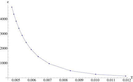
Figure 21: ADM energy density versus horizon temperature ($s=1,\,c_{+}=3$)

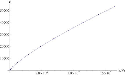
Figure 22: ADM energy density versus entropy density ($s=1,\,c_{+}=50$)

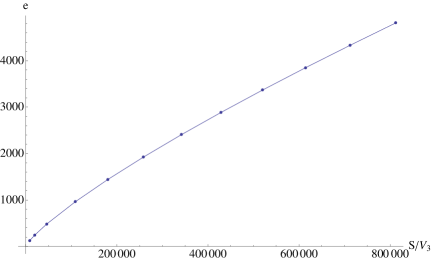
Figure 23: ADM energy density versus entropy density ($s=1,\,c_{+}=3$)

6 Conclusions

Let us summarize what we have done in this paper and point out possible future directions.

• We found finite temperature solutions describing $N_{c}$ D5 branes wrapped on the $S^{2}$ of the resolved conifold. Unlike the generic wrapped D5 branes backgrounds the ones presented here have a dilaton that does not blow up at infinity but stabilizes to a finite value.

• We identify a set of 11 UV and 6 IR parameters that determine the asymptotics of the solutions to any order.

• It was not our goal to explore all the possible families of solutions in the 17 parameter space but to restrict ourselves to those that have a UV behavior similar to the ones in WARPED . Therefore, we fixed several of the UV parameters to appropriate values. We then solved the EOM’s numerically using these UV expansions as boundary conditions and demanding regularity at the horizon. We also imposed that the constraint coming from reparametrization invariance is satisfied, to order $10^{-6}$ or better, throughout all the interval.

• Using U-dualities and these backgrounds as “seeds” we generate solutions with $D3$ and $D5$ charge. To avoid issues related to the uplift of the smeared flavor branes, we show explicitly that after the U-dualities are applied the background obtained is a solution of the EOM’s of $D3$ and $D5$ brane sources.

• In the absence of temperature the backgrounds obtained are dual to interesting field theories that exhibit Seiberg dualities, Higgsing and confinement WARPED . It is tempting to think of the non-extremal solutions found here as dual to finite temperature versions of the field theories in WARPED . However, for non-zero temperature we have to first study the thermodynamical stability. We proceed to do that and find that the specific heat is negative and thus, they are unstable.

• The solutions in HEATING are a particular case (no flavor, $a(\rho)$=0) of ours, thus the thermodynamical instability found here applies also to HEATING .

• We show that our numerical solutions satisfy the First Law of Thermodynamics.

• We find that the temperature grows as the non-extremality parameter decreases. Also, as we increase the area of the horizon the temperature goes to a small non-zero value. A similar behavior was found non-extremal MN GTV and indicates the possibility of a phase transition. It is interesting to pursue this issue further and explore if the dualities can be used to map a phase transition in a wrapped fivebrane background to one in non-extremal KS Buchel:2010wp . Note that the temperature dependence of $F_{(5)}$ and the warp factor necessary to describe the chirally symmetric phase, $T>>T_{c}$, Gubser:2001ri emerges naturally in this framework due to the dualities.

• It would be interesting to study wether there is a connection between our results and the ones existing in the literature regarding non-extremal fractional branes at an orbifold point Bertolini:2002de .

• In Buchel:2005nt it was found that the lowest quasinormal mode in non-extremal Maldacena-Nuñez is tachyonic. In this paper we have studied more general backgrounds than the one inBuchel:2005nt . The negative specific heat seems to indicate that a tachyonic mode is also present in these non-extremal flavored backgrounds, it would be interesting to confirm this.

In WARPED ,Conde:2011aa ,Conde:2011ab ,Elander:2011mh it was shown that solutions of type IIB supergravity with sources generalize the Klebanov-Strassler baryonic branch; the dual field theory exhibits Seiberg dualities, Higgsing and confinement at different scales and was conjectured to describe a mesonic branch. One of the motivations of the present work was to find gravity duals of these interesting field theories. We find that starting from non-extremal wrapped $D5$ branes and applying the same dualities used to generate the extremal backgrounds produces thermodynamically unstable backgrounds. What is then the finite temperature gravity dual of the field theories found in WARPED ,Conde:2011aa ,Conde:2011ab ,Elander:2011mh ? This fascinating question will undoubtedly lead to interesting physics and remains open.

7 Acknowledgments

We thank Carlos Nuñez for many useful discussions, correspondence and comments. We also thank Alex Buchel and Leopoldo Pando Zayas for comments on this manuscript. The work of E.C. and S.Y. is partially supported by the National Science Foundation under Grant No. PHY-0969020. E.C. also acknowledges support of CONACyT grant CB-2008-01-104649 and CONACyT’s High Energy Physics Network.

Appendix A Appendix: The equations of motion

In this appendix we briefly review the metric ansätz and solution method of GTV , which we use to derive the Einstein equations and constraint given in section 2.2 for the flavored non-extremal backgrounds before rotation.

The metric ansätz in GTV , in Einstein frame, reads

$$ds^{2}_{IIB} = -Y_{1}dt^{2}+Y_{2}(dx_{1}^{2}+dx_{2}^{2}+dx_{3}^{2})+Y_{3}d\rho^{2}+Y_{4}(d\theta^{2}+\sin^{2}\theta d\varphi^{2})$$

$$+ Y_{5}\left(\omega_{1}+a\,d\theta)^{2}+(\omega_{2}-a\sin\theta d\varphi)^{2}\right)+Y_{6}(\omega_{3}+\cos\theta d\varphi)^{2}.$$

The $F_{(3)}$ gauge field ansätz is given by

$$F_{(3)} =\frac{N_{c}}{4}\Bigg{[}-(\omega_{1}+b\,d\theta)\wedge(\omega_{2}-b\sin\theta d\varphi)\wedge(\omega_{3}+\cos\theta d\varphi)$$

$$+b^{\prime}dr\wedge(-d\theta\wedge\omega_{1}+\sin\theta d\varphi\wedge\omega_{2})+\left(1-b^{2}-\frac{N_{f}}{N_{c}}\right)\sin\theta d\theta\wedge d\varphi\wedge\omega_{3}\Bigg{]}.$$ (71)

where the $Y_{i}$, $a$, and $b$ are functions of $\rho$ only.
The complete action for type IIB supergravity with smeared flavor branes is then

$$S=S_{\text{grav}}+S_{\text{sources}},$$ (72)

with $S_{\text{grav}}$ and $S_{\text{sources}}$ given by equations (10) and (12).

We plug the metric and $F_{(3)}$ ansätz into this action and integrate over all coordinates except $\rho$, drop the overall volume factor, and end up with a one-dimensional action with Lagrangian

$$L=\sum_{i,j}G_{ij}(Y)Y_{i}^{\prime}Y_{j}^{\prime}-U(Y)\equiv T-U.$$ (73)

We can express the $Y_{i}$ in terms of nine other functions to make $G_{ij}$ diagonal:

$$\begin{array}[]{ccc}Y_{1}=e^{2z-6x},&Y_{2}=e^{2z+2x},&Y_{3}=e^{10y-2z+2l},\\ Y_{4}=e^{2y-2z+2p+2q},&Y_{5}=e^{2y-2z+2p-2q},&Y_{6}=e^{2y-2z-8p},\\ Y_{7}=a,&Y_{8}=b,&Y_{9}=\phi.\end{array}$$ (74)

We end up with the following expressions:

$$T = e^{-l}\left(5y^{\prime 2}-3x^{\prime 2}-2z^{\prime 2}-5p^{\prime 2}-q^{\prime 2}-\frac{1}{4}\,e^{-4q}a^{\prime 2}-\frac{N_{c}^{2}}{64}\,e^{\phi+4z-4y-4p}b^{\prime 2}-\frac{1}{8}\phi^{\prime 2}\right)\,,$$

$$U = \frac{1}{8}\,e^{l}\bigg{[}e^{8y}\left\{e^{-12p}\,[e^{4q}+e^{-4q}(a^{2}-1)^{2}+2a^{2}(1-e^{10p-2q})^{2}]-8e^{-2p}\cosh\ 2q\right\}$$

$$+ \!\!\frac{N_{c}^{2}}{16}e^{\phi+4z+4y+4p}\!\left\{e^{4q}\!+e^{-4q}\!\left(\!a^{2}\!\!-\!2ab+\!1\!-\frac{N_{f}}{N_{c}}\!\right)^{2}\!\!\!+2(a\!-\!b)^{2}\!\right\}\!+\!N_{c}e^{\phi/2+2z+6y-4p}\bigg{]}.$$

Note that the $N_{c}$ dependence can be absorbed by shifting the dilaton, which we will do from now on. We will also write the ratio of the number of flavor branes to color branes as $s\equiv N_{f}/N_{c}$. Since $l$ has no kinetic term, it is a pure gauge degree of freedom reflecting the remaining reparametrization invariance. Varying with respect to $l$ one can set it to any value.

We want to make connection with the metric ansätz given in equation (2.2) in Einstein frame, i.e. one in which

$$\begin{array}[]{ccc}Y_{1}=e^{\phi/2}e^{-8x},&Y_{2}=e^{\phi/2},&Y_{3}=e^{\phi/2}e^{2k}e^{8x},\\ Y_{4}=e^{\phi/2}e^{2h},&Y_{5}=(e^{\phi/2}e^{2g})/4,&Y_{6}=(e^{\phi/2}e^{2k})/4,\\ Y_{7}=a,&Y_{8}=b,&Y_{9}=\phi.\end{array}$$ (76)

In order to do this, we must pick the gauge $l=-4p-4y+4x+\log{2}$, and also make the transformations

$$y=\frac{1}{10}(4g+4h+2k-10x+5\phi-3\log{4}),\;\;p=\frac{1}{10}(g+h-2k+\log{2}),$$

$$q=\frac{1}{2}(-g+h+\log{2}),\;\;z=\frac{1}{4}(-4x+\phi)$$ (77)

After these transformations, the metric ansätz takes the desired form. In practice, we first compute the equations of motion from the Lagrangian in the $p,q,y,z,l,x,\phi$ variables, and then apply the above transformations to get equations of motion in the $k,g,h,x,\phi$ variables. This results in equations (2.2 - 2.2) for the EOMs and constraint, given in section 2.2.

We note that the equations of motion and constraint are invariant under constant shifts of the dilaton

$$\phi\to\phi+C,$$ (78)

as well as shifts in the radial coordinate

$$r\to r+r_{0}.$$ (79)

Appendix B Appendix: UV asymptotics

B.1 Finite temperature UV asymptotics

In the UV, we express the metric and gauge functions as a series in powers of $e^{-2\rho/3}$:

$$e^{2h}= \sum_{i=0}^{\infty}\sum_{j=0}^{i}h_{i,j}\;\rho^{j}\;e^{4(1-i)\rho/3}\quad\quad\quad\quad e^{4\phi}= \sum_{i=1}^{\infty}\sum_{j=0}^{i}f_{i,j}\;\rho^{j}\;e^{4(1-i)\rho/3}$$

$$e^{2g}= \sum_{i=0}^{\infty}\sum_{j=0}^{i}g_{i,j}\;\rho^{j}\;e^{4(1-i)\rho/3} e^{8x}= \sum_{i=1}^{\infty}\sum_{j=0}^{i}x_{i,j}\;\rho^{j}\;e^{2(1-i)\rho/3}$$

$$\ e^{2k}= \sum_{i=0}^{\infty}\sum_{j=0}^{i}k_{i,j}\;\rho^{j}\;e^{4(1-i)\rho/3} a= \sum_{i=1}^{\infty}\sum_{j=0}^{i}a_{i,j}\;\rho^{j}\;e^{2(1-i)\rho/3}$$

$$b= \sum_{i=1}^{\infty}\sum_{j=0}^{i}b_{i,j}\;\rho^{j}\;e^{2(1-i)\rho/3}.$$ (80)

The coefficients $h_{i,j},\cdots,b_{i,j}$ are not all free, and inserting these expansions into the EOMs and constraint equation (2.2 - 2.2) allows us to express them in terms of 11 independent coefficients, which we list here along with their order in the expansion:

$$x_{1,0}\;(\text{const}),\quad x_{5,0}\;(e^{-8\rho/3}),\quad f_{1,0}\;(\text{const}),\quad f_{3,0}\;(e^{-8\rho/3}),$$

$$a_{2,0}\;(e^{-2\rho/3}), a_{4,0}\;(e^{-2\rho}), b_{4,0}\;(e^{-2\rho}),$$

$$k_{0,0}\;(e^{4\rho/3}), k_{3,0}\;(e^{-8\rho/3}),$$

$$h_{1,0}\;(\text{const}), h_{1,1}\;(\rho).$$ (81)

Here we present expressions for the remaining non-zero dependent coefficients in the UV expansions, up to ${\cal O}\left(\text{poly}(\rho)\times e^{-10\rho/3}\right)$. In order to simplify some of the higher order coefficients in what follows, we will assume that $x_{1,0}=1$ and $a_{2,0}=0$.

$\bullet\mathcal{O}(e^{4\rho/3})$:

$$h_{0,0}=\frac{3}{8}k_{0,0}\quad g_{0,0}=\frac{3}{2}k_{0,0}$$ (82)

$\bullet\mathcal{O}(\text{const})$:

$$k_{1,0}=\frac{s}{2},\quad g_{1,0}=\frac{9s}{4}-4h_{1,0},\quad g_{1,1}=-4h_{1,1},$$ (83)

$\bullet\mathcal{O}(e^{-4\rho/3})$:

$$k_{2,0} = \frac{1}{36k_{0,0}}\bigg{(}9+9s^{2}-256h_{1,0}^{2}+9s(-1+16h_{1,0}-9h_{1,1})$$

$$+ 288h_{1,0}h_{1,1}-216h_{1,1}^{2}-\frac{9f_{3,0}k_{0,0}^{2}}{f_{1,0}}\bigg{)}$$

$$k_{2,1} = \frac{3(-2+s)^{2}+8(9s-32h_{1,0})h_{1,1}+144h_{1,1}^{2}}{18k_{0,0}}$$

$$k_{2,2} = -\frac{64h_{1,1}^{2}}{9k_{0,0}}$$

$$g_{2,0} = \frac{1}{24k_{0,0}}\bigg{(}-3+60s^{2}+256h_{1,0}^{2}-3s(11+48h_{1,0}-33h_{1,1})$$

$$- 96h_{1,0}h_{1,1}+120h_{1,1}^{2}-\frac{9f_{3,0}k_{0,0}^{2}}{f_{1,0}}\bigg{)}$$

$$g_{2,1} = \frac{3(-2+s)^{2}+8(-9s+32h_{1,0})h_{1,1}-48h_{1,1}^{2}}{12k_{0,0}}\quad g_{2,2}=\frac{32h_{1,1}^{2}}{3k_{0,0}}$$

$$h_{2,0} = \frac{1}{96k_{0,0}}\bigg{(}-3+24s^{2}+256h_{1,0}^{2}-96h_{1,0}h_{1,1}+120h_{1,1}^{2}$$

$$- 3s(-13+48h_{1,0}+15h_{1,1})-\frac{9f_{3,0}k_{0,0}^{2}}{f_{1,0}}\bigg{)}$$

$$h_{2,1} = \frac{3(-2+s)^{2}+8(-9s+32h_{1,0})h_{1,1}-48h_{1,1}^{2}}{48k_{0,0}}$$

$$h_{2,2} = \frac{8h_{1,1}^{2}}{3k_{0,0}}\quad f_{2,0}=-\frac{2sf_{1,0}}{k_{0,0}}$$ (84)

$\bullet\mathcal{O}(e^{-2\rho})$:

$$b_{4,1}=(2-s)a_{4,0}$$ (85)

$\bullet\mathcal{O}(e^{-8\rho/3})$:

$$k_{3,1} = \frac{1}{432f_{1,0}k_{0,0}^{2}}\Bigg{[}sf_{1,0}\bigg{[}103s^{2}-4s(-125+352h_{1,0}+304h_{1,1})$$

$$+ 4\Big{(}1+1024h_{1,0}^{2}+64h_{1,0}(-7+25h_{1,1})+4h_{1,1}(-73+91h_{1,1})\Big{)}\bigg{]}$$

$$+ 24s(x_{5,0}f_{1,0}-f_{3,0})k_{0,0}^{2}+576f_{1,0}k_{0,0}^{3}a_{4,0}^{2}\Bigg{]}$$

$$k_{3,2} = \frac{s\bigg{[}(-2+s)^{2}-8(14+11s-64h_{1,0})h_{1,1}+400h_{1,1}^{2}\bigg{]}}{54k_{0,0}^{2}}$$

$$k_{3,3} = \frac{256sh_{1,1}^{2}}{81k_{0,0}^{2}}$$

$$g_{3,0} = -x_{5,0}h_{1,0}+\frac{f_{3,0}h_{1,0}}{f_{1,0}}+\frac{3}{4}x_{5,0}h_{1,1}+s^{2}\bigg{(}-\frac{313}{192k_{0,0}^{2}}-\frac{5h_{1,0}}{3k_{0,0}^{2}}+\frac{373h_{1,1}}{96k_{0,0}^{2}}\bigg{)}$$

$$+ s\bigg{(}\frac{5}{8}x_{5,0}-\frac{f_{3,0}}{2f_{1,0}}+\frac{313}{192k_{0,0}^{2}}+\frac{2h_{1,0}}{k_{0,0}^{2}}-\frac{8h_{1,0}^{2}}{3k_{0,0}^{2}}-\frac{79h_{1,1}}{48k_{0,0}^{2}}-\frac{35h_{1,0}h_{1,1}}{3k_{0,0}^{2}}-\frac{131h_{1,1}^{2}}{48k_{0,0}^{2}}\bigg{)}$$

$$+ \frac{1225s^{3}}{768k_{0,0}^{2}}-\frac{7h_{1,0}}{3k_{0,0}^{2}}-\frac{7h_{1,1}}{4k_{0,0}^{2}}+\frac{32h_{1,0}^{2}h_{1,1}}{3k_{0,0}^{2}}+\frac{40h_{1,0}h_{1,1}^{2}}{3k_{0,0}^{2}}+\frac{7h_{1,1}^{3}}{k_{0,0}^{2}}-\frac{3}{4}k_{3,0}+\frac{3}{8}k_{0,0}a_{4,0}^{2}$$

$$g_{3,1} = -x_{5,0}h_{1,1}+\frac{f_{3,0}h_{1,1}}{f_{1,0}}+s^{2}\bigg{(}-\frac{317}{144k_{0,0}^{2}}+\frac{16h_{1,0}}{9k_{0,0}^{2}}+\frac{4h_{1,1}}{9k_{0,0}^{2}}\bigg{)}$$

$$+ s\bigg{(}-\frac{1}{24}x_{5,0}+\frac{f_{3,0}}{24f_{1,0}}+\frac{191}{144k_{0,0}^{2}}+\frac{52h_{1,0}}{9k_{0,0}^{2}}-\frac{64h_{1,0}^{2}}{9k_{0,0}^{2}}+\frac{145h_{1,1}}{36k_{0,0}^{2}}$$

$$- \frac{148h_{1,0}h_{1,1}}{9k_{0,0}^{2}}-\frac{511h_{1,1}^{2}}{36k_{0,0}^{2}}\bigg{)}$$

$$+ \frac{89s^{3}}{576k_{0,0}^{2}}-\frac{8h_{1,0}}{3k_{0,0}^{2}}-\frac{7h_{1,1}}{3k_{0,0}^{2}}+\frac{64h_{1,0}h_{1,1}^{2}}{3k_{0,0}^{2}}+\frac{40h_{1,1}^{3}}{3k_{0,0}^{2}}-k_{0,0}a_{4,0}^{2}$$

$$g_{3,2} = s^{2}\bigg{(}\frac{1}{18k_{0,0}^{2}}+\frac{5h_{1,1}}{9k_{0,0}^{2}}\bigg{)}+s\bigg{(}-\frac{1}{18k_{0,0}^{2}}+\frac{38h_{1,1}}{9k_{0,0}^{2}}-\frac{64h_{1,0}h_{1,1}}{9k_{0,0}^{2}}-\frac{74h_{1,1}^{2}}{9k_{0,0}^{2}}\bigg{)}$$

$$- \frac{s^{3}}{72k_{0,0}^{2}}-\frac{8h_{1,1}}{3k_{0,0}^{2}}+\frac{32h_{1,1}^{3}}{3k_{0,0}^{2}}$$

$$g_{3,3} = -\frac{64sh_{1,1}^{2}}{27k_{0,0}^{2}}$$

$$h_{3,0} = \frac{1}{4}x_{5,0}h_{1,0}-\frac{f_{3,0}h_{1,0}}{4f_{1,0}}-\frac{3}{16}x_{5,0}h_{1,1}+s^{2}\bigg{(}-\frac{25}{768k_{0,0}^{2}}+\frac{5h_{1,0}}{4k_{0,0}^{2}}+\frac{259h_{1,1}}{384k_{0,0}^{2}}\bigg{)}$$

$$+ s\bigg{(}\frac{1}{64}x_{5,0}+\frac{f_{3,0}}{64f_{1,0}}+\frac{61}{768k_{0,0}^{2}}-\frac{2h_{1,0}}{3k_{0,0}^{2}}-\frac{2h_{1,0}^{2}}{3k_{0,0}^{2}}-\frac{247h_{1,1}}{192k_{0,0}^{2}}+\frac{h_{1,0}h_{1,1}}{12k_{0,0}^{2}}+\frac{229h_{1,1}^{2}}{192k_{0,0}^{2}}\bigg{)}$$

$$- \frac{287s^{3}}{3072k_{0,0}^{2}}+\frac{7h_{1,0}}{12k_{0,0}^{2}}+\frac{7h_{1,1}}{16k_{0,0}^{2}}-\frac{8h_{1,0}^{2}h_{1,1}}{3k_{0,0}^{2}}-\frac{10h_{1,0}h_{1,1}^{2}}{3k_{0,0}^{2}}-\frac{7h_{1,1}^{3}}{4k_{0,0}^{2}}$$

$$- \frac{3}{16}k_{3,0}-\frac{9}{32}k_{0,0}a_{4,0}^{2}$$

$$h_{3,1} = \frac{1}{4}x_{5,0}h_{1,1}-\frac{f_{3,0}h_{1,1}}{4f_{1,0}}+s^{2}\bigg{(}-\frac{101}{576k_{0,0}^{2}}+\frac{7h_{1,0}}{9k_{0,0}^{2}}+\frac{16h_{1,1}}{9k_{0,0}^{2}}\bigg{)}$$

$$+ s\bigg{(}-\frac{1}{96}x_{5,0}+\frac{f_{3,0}}{96f_{1,0}}-\frac{25}{576k_{0,0}^{2}}+\frac{h_{1,0}}{9k_{0,0}^{2}}-\frac{16h_{1,0}^{2}}{9k_{0,0}^{2}}$$

$$- \frac{23h_{1,1}}{144k_{0,0}^{2}}-\frac{37h_{1,0}h_{1,1}}{9k_{0,0}^{2}}-\frac{79h_{1,1}^{2}}{144k_{0,0}^{2}}\bigg{)}$$

$$- \frac{127s^{3}}{2304k_{0,0}^{2}}+\frac{2h_{1,0}}{3k_{0,0}^{2}}+\frac{7h_{1,1}}{12k_{0,0}^{2}}-\frac{16h_{1,0}h_{1,1}^{2}}{3k_{0,0}^{2}}-\frac{10h_{1,1}^{3}}{3k_{0,0}^{2}}-\frac{1}{4}k_{0,0}a_{4,0}^{2}$$

$$h_{3,2} = s^{2}\bigg{(}\frac{1}{72k_{0,0}^{2}}+\frac{17h_{1,1}}{36k_{0,0}^{2}}\bigg{)}+s\bigg{(}-\frac{1}{72k_{0,0}^{2}}-\frac{5h_{1,1}}{18k_{0,0}^{2}}-\frac{16h_{1,0}h_{1,1}}{9k_{0,0}^{2}}-\frac{37h_{1,1}^{2}}{18k_{0,0}^{2}}\bigg{)}$$

$$- \frac{s^{3}}{288k_{0,0}^{2}}+\frac{2h_{1,1}}{3k_{0,0}^{2}}-\frac{8h_{1,1}^{3}}{3k_{0,0}^{2}}$$

$$h_{3,3} = -\frac{16sh_{1,1}^{2}}{27k_{0,0}^{2}}\quad f_{3,1}=-\frac{8f_{1,0}}{3k_{0,0}^{2}}+\frac{8sf_{1,0}}{3k_{0,0}^{2}}-\frac{2s^{2}f_{1,0}}{3k_{0,0}^{2}}$$ (86)

$\bullet\mathcal{O}(e^{-10\rho/3})$:

$$a_{6,0} = -\frac{3sa_{4,0}}{4k_{0,0}}+\frac{8h_{1,0}a_{4,0}}{3k_{0,0}}\quad a_{6,1}=\frac{8h_{1,1}a_{4,0}}{3k_{0,0}}$$

$$b_{6,0} = \frac{33s^{2}a_{4,0}}{128k_{0,0}}+s\bigg{(}\frac{3b_{4,0}}{8k_{0,0}}+\frac{21a_{4,0}}{64k_{0,0}}-\frac{3h_{1,0}a_{4,0}}{2k_{0,0}}-\frac{45h_{1,1}a_{4,0}}{32k_{0,0}}\bigg{)}$$

$$b_{6,1} = -\frac{3s^{2}a_{4,0}}{8k_{0,0}}+s\bigg{(}\frac{3a_{4,0}}{4k_{0,0}}-\frac{3h_{1,1}a_{4,0}}{2k_{0,0}}\bigg{)}$$ (87)

B.2 Supersymmetric UV asymptotics

Here we summarize the BPS, zero-temperature UV asymptotics (up to $\mathcal{O}(e^{-4\rho/3})$) of the backgrounds corresponding to D5s wrapped on the $S^{2}$ of the resolved conifold, with the addition of smeared D5 flavor sources, as described in HoyosBadajoz:2008fw ; WARPED . These serve as matching conditions for our finite temperature UV asymptotics. In addition, they furnish us with a family of reference backgrounds that are used in the energy calculations of section 5.

The BPS asymptotics are given in terms of the free variables $Q_{0},c_{+},c_{-},\rho_{0}$ and $f_{1,0}$ after performing a UV expansion of e.g. equations (3.5) of WARPED . The finite temperature asymptotics of section 3.1 are a deformation of these BPS asymptotics with $\rho_{0}=0,\ Q_{0}=-N_{c}+N_{f}/2$ and $f_{1,0}=1$. In the energy calculations of section 5, we also set $\rho_{0}=0$, but $Q_{0},\ c_{+},\ c_{-}$ and $f_{1,0}$ are left free to allow for the matching.

What follows, then, is the form of the UV BPS asymptotics with $\rho_{0}=0$, but with $Q_{0},\ c_{+},\ c_{-}$ and $f_{1,0}$ left free.

$$e^{2k} = \frac{2}{3}c_{+}e^{4\rho/3}+\frac{s}{2}+\frac{1}{96c_{+}}e^{-4\rho/3}\bigg{[}-64Q_{0}^{2}-16(3-4\rho)^{2}+16s(3-4\rho)^{2}$$

$$+32Q_{0}(-2+s)(-3+4\rho)+s^{2}\left(-27+96\rho-64\rho^{2}\right)\bigg{]}$$

$$e^{2h} = \frac{1}{4}c_{+}e^{4\rho/3}+\frac{1}{32}\left(8Q_{0}+9s-8(-2+s)\rho\right)$$

$$+\frac{1}{256c_{+}}e^{-4\rho/3}\bigg{[}64Q_{0}^{2}+9\left(16-16s+3s^{2}\right)-128Q_{0}(-2+s)\rho+64(-2+s)^{2}\rho^{2}\bigg{]}$$

$$e^{2g} = c_{+}e^{4\rho/3}-Q_{0}+\frac{9s}{8}+(-2+s)\rho$$

$$+\frac{1}{64c_{+}}e^{-4\rho/3}\bigg{[}64Q_{0}^{2}+9\left(16-16s+3s^{2}\right)-128Q_{0}(-2+s)\rho+64(-2+s)^{2}\rho^{2}\bigg{]}$$

$$e^{4\phi} = f_{10}-\frac{3e^{-4\rho/3}sf_{10}}{c_{+}}+\frac{3f_{1,0}}{8c_{+}^{2}}e^{-8\rho/3}\bigg{[}4Q_{0}(-2+s)+s^{2}(15-4\rho)-2(3+8\rho)+2s(3+8\rho)\bigg{]}$$

$$a = 2e^{-2\rho}\;\;\;\;\;\;\;\;\;\;b=e^{-2\rho}(2+2Q_{0}-s-2(-2+s)\rho)$$ (88)

Appendix C Appendix: Comments on numerical procedure

The UV-shot solutions of section 3.3 were obtained by using Mathematica’s NDSolve, with UV boundary conditions determined by the expansions given in equation (B.1) up to $\mathcal{O}(e^{-8\rho})$ for $e^{8x}$, $\mathcal{O}(e^{-26\rho/3})$ for $a$ and $b$, $\mathcal{O}(e^{-20\rho/3})$ for $e^{2k},e^{2g}$ and $e^{2h}$, and $\mathcal{O}(e^{-8\rho})$ for $e^{4\phi}$. Using an expansion taken out to this order, NDSolve at WorkingPrecision = 70 finds a horizon radius $\rho_{h}$ which is fairly independent of the value of $\rho_{\infty}$ chosen ($\sim$ 1 part in $10^{-5}$ as $\rho_{\infty}$ is varied from 6 to 9). The constraint equation (2.2) is of order $10^{-8}$ when evaluated on a typical UV-shot solution, but climbs near the horizon; on the horizon shot solution the constraint is of order $10^{-14}$ with a maximum of $\sim 10^{-6}$ at the horizon — see Figs. (26) and (26). The degree to which the constraint equation is violated near the horizon also depends on the size of $C_{2}$. This stems from the fact that many higher order terms in the UV expansion are proportional to $C_{2}$, so any finite order truncation of the UV asymptotics becomes less accurate for larger $C_{2}$ values.

When matching our UV-shot solutions to a series expansion near the horizon, we choose to exclude the $a$ and $b$ functions, the dilaton, and their derivatives from the mismatch function. The reason for excluding the $a$ and $b$ functions is that unlike the metric and dilaton functions — whose UV and horizon shot solutions agree quite well away from the horizon in what NMinimize considers the best matched case — $a$ and $b$’s UV and horizon shot solutions differ over the entire interval in the best matched case, as shown in Fig. (26) (although $a$ and $b$ are typically small in magnitude compared to $x,g,h,k\text{\ and\ }\phi$). The UV-shot dilaton also displays divergent behavior near the horizon, and drastically decreases the match’s accuracy if included. Including it in the match also produces a horizon-shot dilaton which stabilizes to a UV value different than $e^{4\phi}|_{\rho_{\infty}}\sim 1$. We remedy this by using the invariance of the EOMs under a constant shift in the dilaton. After the matching is performed, we pick an $f_{0}$ that gives a horizon-shot dilaton that agrees with the UV value of $e^{4\phi}|_{\rho_{\infty}}\sim 1$. For the solutions we have found, including $a$, $b$ and the dilaton allows for the mismatch to be minimized to only $\sim 10^{-2}$, and the resulting horizon shot solutions for $(x,g,h,k,f)$ differ significantly from the UV shot solutions. Excluding $a$, $b$ and $\phi$ from the mismatch function, NMinimize is able to reduce the mismatch to $\sim 10^{-7}$, and the resulting horizon shot solutions for $(x,g,h,k,\phi,a)$ agree very closely with the UV shot solutions. This will still leave us with a horizon-shot $b$ that tends to exponentially diverging behavior at large $\rho$. However, $b_{0}$ can be tuned to eliminate this divergence, with negligible effect on the behavior of the other functions $(x,g,h,k,f)$ — see Fig. (26).

Performing our matching close to the horizon (e.g. $\epsilon=.15$) necessarily involves greater errors in the UV-shot solutions. This shows up as horizon-shot solutions that disagree with the UV-shot solutions near $\rho_{\infty}$. To remedy this, we instead begin by matching at a higher $\epsilon=.7$ — this eliminates the disagreement near $\rho_{\infty}$. We then use the resulting values of the matched horizon parameters as seeds for a new match performed at a lower $\epsilon=.15$, where in addition we constrain the allowed variance of $(x_{1},g_{0},h_{0},k_{0},f_{0})$ around the seed values until the resulting $\epsilon=.15$ match gives horizon shot solutions which agree with the UV shot solutions at $\rho_{\infty}$. After doing this, we find that the high-$\epsilon$-seeded $\epsilon=.15$ match produces a mismatch of the same order ($10^{-7}$) as a non-seeded $\epsilon=.15$ match, with the added benefit that the high-$\epsilon$-seeded horizon-shot solutions are in good agreement with the UV-shot solutions at $\rho_{\infty}$

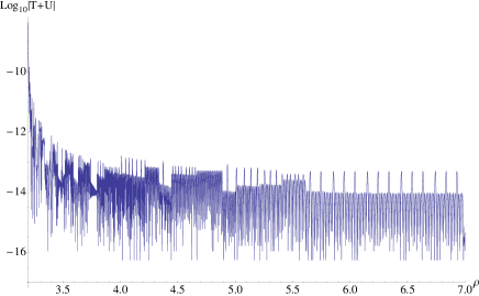
Figure 24: Constraint evaluated on a horizon shot solution with $c_{+}=50,C_{2}=5000,s=1$.

Figure 25: Constraint evaluated on same solution, near horizon at $\rho_{h}\simeq 3.194024.$

Figure 26: Horizon-shot and UV-shot $a$ and $b$ after tuning $b_{0}$. brown - UV-shot $a$, black - UV-shot $b$, blue - horizon shot $a$, red - horizon-shot $b$. $s=1$, $c=3$, $C_{2}=800000$.

The numerical method we use could undoubtedly be improved. However, as presented here it is enough to identify the behavior of the horizon temperature as a function of the non-extremality parameter $C_{2}$, which is necessary to study the stability of the background. Other methods have been used, such as Mahato:2007zm .

Appendix D Appendix: U-Duality for the flavored, wrapped D5 branes black hole

Here we describe in more detail the steps of the U-duality procedure as applied to backgrounds of the type mentioned in equations (2.2) and (LABEL:eq:F3ansatz). We will consider the rotation in string frame. We begin with

$$ds^{2}_{IIB} = e^{\phi(\rho)}\Big{[}-e^{-8x(\rho)}dt^{2}+dx_{1}^{2}+dx_{2}^{2}+dx_{3}^{2}\Big{]}+ds_{6}^{2},$$

$$ds_{6}^{2} = e^{\phi(\rho)}\Big{[}e^{8x(\rho)}e^{2k(\rho)}d\rho^{2}+e^{2h(\rho)}(d\theta^{2}+\sin^{2}\theta d\varphi^{2})$$ (89)

$$+ \frac{e^{2g(\rho)}}{4}\left((\omega_{1}+a(\rho)d\theta)^{2}+(\omega_{2}-a(\rho)\sin\theta d\varphi)^{2}\right)$$

$$+ \frac{e^{2k(\rho)}}{4}(\omega_{3}+\cos\theta d\varphi)^{2}\Big{]},$$

and

$$F_{(3)} = \frac{N_{c}}{4}\Bigg{[}-(\omega_{1}+b(\rho)d\theta)\wedge(\omega_{2}-b(\rho)\sin\theta d\varphi)\wedge(\omega_{3}+\cos\theta d\varphi)+$$

$$b^{\prime}d\rho\wedge(-d\theta\wedge\omega_{1}+\sin\theta d\varphi\wedge\omega_{2})+(1-b(\rho)^{2}-\frac{N_{f}}{N_{c}})\sin\theta d\theta\wedge d\varphi\wedge\omega_{3}\Bigg{]}.$$

We will supress obvious $\rho$ dependence to avoid cluttering. We begin by T-dualizing in the $x_{1},x_{2},x_{3}$ directions, which results in the type IIA background

$$ds^{2}_{IIA}=e^{\phi}\Big{[}-e^{-8x}dt^{2}\Big{]}+e^{-\phi}(dx_{1}^{2}+dx_{2}^{2}+dx_{3}^{2})+ds_{6}^{2},$$

$$e^{2\phi_{A}}=e^{-\phi},$$

$$F_{(6)}=F_{(3)}\wedge dx_{1}\wedge dx_{2}\wedge dx_{3}\to F_{(4)}=e^{2\phi}e^{-4x}*_{6}F_{(3)}\wedge dt.$$ (91)

where

$$*_{6}F_{(3)}=\frac{N_{c}e^{4x}}{8}\Bigg{\{} -\Big{[}e^{2g-2h}a^{2}\left(1+a^{2}-2ab-s\right)+16e^{2h-2g}+8a\left(a-b\right)\Big{]}e_{1}\wedge e_{2}\wedge d\rho$$ (92)

$$+\Big{[}e^{2g-2h}a\left(1+a^{2}-2ab-s\right)+4(a-b)\Big{]}\left(e_{1}\wedge\omega_{2}+e_{2}\wedge\omega_{1}\right)\wedge d\rho$$

$$+e^{2g-2h}\left(1+a^{2}-2ab-s\right)\left(\omega_{1}\wedge\omega_{2}\wedge d\rho\right)$$

$$+e^{-8x}\,b^{\prime}\left(e_{1}\wedge\omega_{1}+e_{2}\wedge\omega_{2}\right)\wedge\tilde{\omega}_{3}\Bigg{\}}.$$

Now, we lift this to M-theory:

$$ds^{2}_{11}=e^{-2\phi/3}dx_{11}^{2}+e^{\phi/3}\Big{[}-e^{-8x}e^{\phi}dt^{2}+e^{-\phi}(dx_{1}^{2}+dx_{2}^{2}+dx_{3}^{2})+ds_{6}^{2}\Big{]},$$

$$G_{(4)}=e^{-4x}e^{2\phi}*_{6}F_{(3)}\wedge dt.$$ (93)

Boosting in the $(t,x_{11})$ directions according to

$$dt\to\cosh\beta dt-\sinh\beta dx_{11},\;\;\;\;dx_{11}\to-\sinh\beta dt+\cosh\beta dx_{11},$$ (94)

we rewrite the boosted metric as

$$ds^{2}_{11}=e^{\phi/3}\Big{[}e^{-\phi}(dx_{1}^{2}+dx_{2}^{2}+dx_{3}^{2})+ds_{6}^{2}\Big{]}+Adt^{2}+Bdx_{11}^{2}+Cdtdx_{11},$$

$$G_{(4)}=e^{-4x}e^{2\phi}*_{6}F_{(3)}\Big{[}\cosh\beta dt-\sinh\beta dx_{11}\Big{]}$$ (95)

where

$$A=e^{4\phi/3}[\sinh^{2}\beta e^{-2\phi}-e^{-8x}\cosh^{2}\beta],\;\;B=e^{4\phi/3}[\cosh^{2}\beta e^{-2\phi}-e^{-8x}\sinh^{2}\beta],$$

$$C=-2\cosh\beta\sinh\beta e^{4\phi/3}[e^{-2\phi}-e^{-8x}].$$ (96)

Before reducing to IIA, it is useful to write equation (95) as

$$ds^{2}_{11}=B^{-1/2}\Big{[}g_{tt}dt^{2}+B^{1/2}e^{\phi/3}(e^{-\phi}(dx_{1}^{2}+dx_{2}^{2}+dx_{3}^{2})+ds_{6}^{2})\Big{]}+B(dx_{11}+a_{t}dt)^{2},$$

$$G_{(4)}=e^{-4x}e^{2\phi}*_{6}F_{(3)}\Big{[}(\cosh\beta+a_{t}\sinh\beta)dt-\sinh\beta(dx_{11}+a_{t}dt)\Big{]}$$ (97)

where we have defined

$$a_{t}=\frac{C}{2B},\;\;\;\;g_{tt}=\frac{4AB-C^{2}}{4\sqrt{B}},\;\;e^{4\phi_{A}/3}=B.$$ (98)

Now we reduce to IIA, obtaining in string frame,

$$ds^{2}_{IIA}=g_{tt}dt^{2}+\sqrt{B}e^{-2\phi/3}(dx_{1}^{2}+dx_{2}^{2}+dx_{3}^{2})+\sqrt{B}e^{\phi/3}ds_{6}^{2},$$

$$e^{2\phi_{A}}=B^{3/2},$$

$$F_{(4)}=e^{-4x}e^{2\phi}*_{6}F_{(3)}\wedge\Big{[}(\cosh\beta+a_{t}\sinh\beta)dt\Big{]},$$

$$H_{(3)}=-\sinh\beta\,e^{-4x}e^{2\phi}*_{6}F_{(3)},$$

$$F_{(2)}=a_{t}^{\prime}d\rho\wedge dt.$$ (99)

Next, we T-dualize back along the $x_{1},x_{2},x_{3}$ directions, and obtain

$$ds^{2}_{IIB}=g_{tt}dt^{2}+\frac{e^{2\phi/3}}{\sqrt{B}}(dx_{3}^{2}+dx_{1}^{2}+dx_{2}^{2})+\sqrt{B}e^{\phi/3}ds_{6}^{2},$$

$$e^{2\phi_{B}}=e^{2\phi},$$

$$F_{(7)}=e^{-4x}e^{2\phi}*_{6}F_{(3)}\wedge\Big{[}(\cosh\beta+a_{t}\sinh\beta)dt\Big{]}\wedge dx_{3}\wedge dx_{2}\wedge dx_{1}\quad\quad F_{(3)}=*_{10}F_{7},$$

$$H_{(3)}=-\sinh\beta\,e^{-4x}e^{2\phi}*_{6}F_{(3)},$$

$$F_{(5)}=a_{t}^{\prime}d\rho\wedge dt\wedge dx_{3}\wedge dx_{2}\wedge dx_{1}(1+*_{10}).$$ (100)

Finally we use the definitions for $A,B,C$ and $a_{t}$, and take the limit $\beta\to\infty$. This is the field theory limit, where the warp factors vanish at infinity. We then rescale

$$\tilde{N}=N\cosh\beta,\qquad x_{i}\to\sqrt{\cosh\beta}\sqrt{\tilde{N}\alpha^{\prime}}x_{i}.$$ (101)

With all of the above, the $\beta\to\infty$ limits are finite and the final solution is given by equations (35) and (36) after transforming to Einstein frame .

Appendix E Appendix: General form of $B_{2}$

In the extremal case WARPED , the $SU(3)$ structure fixes the form of $B_{(2)}$. In our solutions $B_{(2)}$ should reduce to the one in WARPED when $T=0$. The following ansätz is compatible with that requirement:

$$B_{(2)}=b_{1}(\rho)\tilde{\omega_{3}}\wedge d\rho+b_{2}(\rho)e_{1}\wedge e_{2}+b_{3}(\rho)e_{1}\wedge\tilde{\omega}_{2}+b_{4}(\rho)e_{2}\wedge\tilde{\omega}_{1}+b_{5}(\rho)\tilde{\omega}_{1}\wedge\tilde{\omega}_{2}.$$ (102)

We find it convenient to introduce a new function $\widetilde{b_{2}}(\rho)$ and parametrize $b_{2}$ as,

$$b_{2}(\rho)=\widetilde{b_{2}}(\rho)+(1-a(\rho)^{2})b_{5}(\rho)$$ (103)

Therefore,

$$\ B_{(2)}=b_{1}(\rho)\tilde{\omega_{3}}\wedge d\rho+(\widetilde{b_{2}}(\rho)+(1-a(\rho)^{2})b_{5}(\rho))e_{1}\wedge e_{2}+b_{3}(\rho)e_{1}\wedge\tilde{\omega}_{2}+b_{4}(\rho)e_{2}\wedge\tilde{\omega}_{1}+b_{5}(\rho)\tilde{\omega}_{1}\wedge\tilde{\omega}_{2}.$$ (104)

With this notation it is easy to show that

$$B_{(2)}=B_{(2)}|_{b_{5}=0}-d\left[b_{5}(\rho)\tilde{\omega_{3}}\right]$$ (105)

Thus, $b_{5}$ is really a gauge choice that does not affect the value of $H_{(3)}$.

From (35) we have,

$$H_{(3)} =-e^{-4x}\frac{1}{4}\,e^{2\phi}\,*_{6}\,f_{(3)}$$

Demanding that $H_{(3)}=d[B_{(2)}]$ results in five equations,

$$\cot(\theta)(b_{3}-b_{4})=0$$

$$b_{3}+ab_{5}-\frac{1}{8}e^{2\phi-8x}b^{\prime}=0$$

$$2e^{2\phi-2g+2h}-(-1+a^{2})b_{1}+(b_{3}+b_{4}+2ab_{5})a^{\prime}-\widetilde{b_{2}}^{\prime}-b_{5}^{\prime}(1-a^{2})=0$$

$$e^{2\phi}(-a+b)-2(ab_{1}+b_{5}a^{\prime}+b_{3}^{\prime})=0$$

$$\frac{1}{8}e^{2\phi+2g-2h}\left(-1+s-a^{2}+2ab\right)+b_{1}-b_{5}^{\prime}=0$$ (107)

Three of them are easily solved by setting,

$$b_{3}=b_{4}$$

$$b_{4}=-\frac{1}{8}\left(8ab_{5}-e^{2\phi-8x}b^{\prime}\right)$$

$$b_{1}=\frac{1}{8}e^{-2h+2g+2\phi}\left(1-s+a^{2}-2ab\right)+b_{5}^{\prime}=0$$ (108)

we are then left with two equations, one of them is just the equation of motion for $b(\rho)$. The other one is a differential equation for $\widetilde{b_{2}}(\rho)$,

$$e^{2\phi+4g+8x}\left(sa^{2}-a^{4}-2ab+2a^{3}b)\right) +e^{2\phi+2g+2h}a^{\prime}b^{\prime}+e^{8x+2\phi}\left(16e^{4h}-e^{4g}(-1+s)\right)$$

$$\qquad-e^{8x+2g+2h}\widetilde{b_{2}}^{\prime}(\rho)=0$$ (109)

Note that equations (E-E) determine $B_{2}$ in terms of an arbitrary function $b_{5}$ that we have shown is just a gauge choice. In order to make contact with WARPED we choose,

$$b_{5}^{\prime}=\frac{1}{8}e^{2\phi-2h}\left(4e^{2h+2k}+e^{2g}(-1+s-a^{2}+2ab)\right)$$ (110)

which gives $b_{1}=\frac{1}{2}e^{2\phi+2k}$.

References

- (1) J. M. Maldacena, The Large N limit of superconformal field theories and supergravity, Adv.Theor.Math.Phys. 2 (1998) 231–252, [hep-th/9711200].
- (2) S. Gubser, I. R. Klebanov, and A. M. Polyakov, Gauge theory correlators from noncritical string theory, Phys.Lett. B428 (1998) 105–114, [hep-th/9802109].
- (3) E. Witten, Anti-de Sitter space and holography, Adv.Theor.Math.Phys. 2 (1998) 253–291, [hep-th/9802150].
- (4) I. R. Klebanov and M. J. Strassler, Supergravity and a confining gauge theory: Duality cascades and chi SB resolution of naked singularities, JHEP 0008 (2000) 052, [hep-th/0007191].
- (5) J. M. Maldacena and C. Nunez, Towards the large N limit of pure N = 1 super Yang Mills, Phys. Rev. Lett. 86 (2001) 588–591, [hep-th/0008001].
- (6) G. Papadopoulos and A. A. Tseytlin, Complex geometry of conifolds and five-brane wrapped on two sphere, Class.Quant.Grav. 18 (2001) 1333–1354, [hep-th/0012034].
- (7) A. Butti, M. Grana, R. Minasian, M. Petrini, and A. Zaffaroni, The baryonic branch of Klebanov-Strassler solution: A supersymmetric family of SU(3) structure backgrounds, JHEP 03 (2005) 069, [hep-th/0412187].
- (8) R. Casero, C. Nunez, and A. Paredes, Towards the string dual of N=1 SQCD-like theories, Phys.Rev. D73 (2006) 086005, [hep-th/0602027].
- (9) F. Benini, F. Canoura, S. Cremonesi, C. Nunez, and A. V. Ramallo, Unquenched flavors in the Klebanov-Witten model, JHEP 0702 (2007) 090, [hep-th/0612118].
- (10) E. Caceres, R. Flauger, M. Ihl, and T. Wrase, New supergravity backgrounds dual to N=1 SQCD-like theories with N(f) = 2N(c), JHEP 0803 (2008) 020, [arXiv:0711.4878].
- (11) F. Bigazzi, A. L. Cotrone, and A. Paredes, Klebanov-Witten theory with massive dynamical flavors, JHEP 0809 (2008) 048, [arXiv:0807.0298].
- (12) C. Nunez, A. Paredes, and A. V. Ramallo, Unquenched Flavor in the Gauge/Gravity Correspondence, Adv.High Energy Phys. 2010 (2010) 196714, [arXiv:1002.1088].
- (13) F. Benini, F. Canoura, S. Cremonesi, C. Nunez, and A. V. Ramallo, Backreacting flavors in the Klebanov-Strassler background, JHEP 0709 (2007) 109, [arXiv:0706.1238].
- (14) F. Bigazzi, A. L. Cotrone, A. Paredes, and A. V. Ramallo, The Klebanov-Strassler model with massive dynamical flavors, JHEP 0903 (2009) 153, [arXiv:0812.3399].
- (15) J. Maldacena and D. Martelli, The Unwarped, resolved, deformed conifold: Fivebranes and the baryonic branch of the Klebanov-Strassler theory, JHEP 1001 (2010) 104, [arXiv:0906.0591].
- (16) J. Gaillard, D. Martelli, C. Nunez, and I. Papadimitriou, The warped, resolved, deformed conifold gets flavoured, Nucl. Phys. B843 (2011) 1–45, [arXiv:1004.4638].
- (17) E. Conde, J. Gaillard, C. Nunez, M. Piai, and A. V. Ramallo, A Tale of Two Cascades: Higgsing and Seiberg-Duality Cascades from type IIB String Theory, JHEP 1202 (2012) 145, [arXiv:1112.3350].
- (18) E. Conde, J. Gaillard, C. Nunez, M. Piai, and A. V. Ramallo, Towards the String Dual of Tumbling and Cascading Gauge Theories, Phys.Lett. B709 (2012) 385–389, [arXiv:1112.3346]. 7 pages, 6 figures / v2. minor changes included.
- (19) D. Elander, J. Gaillard, C. Nunez, and M. Piai, Towards multi-scale dynamics on the baryonic branch of Klebanov-Strassler, JHEP 1107 (2011) 056, [arXiv:1104.3963].
- (20) S. Bennett, E. Caceres, C. Nunez, D. Schofield, and S. Young, The Non-SUSY Baryonic Branch: Soft Supersymmetry Breaking of N=1 Gauge Theories, JHEP 1205 (2012) 031, [arXiv:1111.1727].
- (21) E. Caceres, C. Nunez, and L. A. Pando-Zayas, Heating up the Baryonic Branch with U-duality: A Unified picture of conifold black holes, JHEP 1103 (2011) 054, [arXiv:1101.4123].
- (22) A. Buchel, Chiral symmetry breaking in cascading gauge theory plasma, Nucl.Phys. B847 (2011) 297–324, [arXiv:1012.2404].
- (23) O. Aharony, A. Buchel, and P. Kerner, The Black hole in the throat: Thermodynamics of strongly coupled cascading gauge theories, Phys.Rev. D76 (2007) 086005, [arXiv:0706.1768].
- (24) M. Mahato, L. A. Pando Zayas, and C. A. Terrero-Escalante, Black Holes in Cascading Theories: Confinement/Deconfinement Transition and other Thermal Properties, JHEP 0709 (2007) 083, [arXiv:0707.2737].
- (25) S. S. Gubser, A. A. Tseytlin, and M. S. Volkov, NonAbelian 4-d black holes, wrapped five-branes, and their dual descriptions, JHEP 0109 (2001) 017, [hep-th/0108205].
- (26) A. Buchel, Hydrodynamics of the cascading plasma, Nucl.Phys. B820 (2009) 385–416, [arXiv:0903.3605].
- (27) S. Gubser, C. Herzog, I. R. Klebanov, and A. A. Tseytlin, Restoration of chiral symmetry: A Supergravity perspective, JHEP 0105 (2001) 028, [hep-th/0102172].
- (28) C. Hoyos-Badajoz, C. Nunez, and I. Papadimitriou, Comments on the String dual to N=1 SQCD, Phys.Rev. D78 (2008) 086005, [arXiv:0807.3039].
- (29) J. M. Maldacena and C. Nunez, Supergravity description of field theories on curved manifolds and a no go theorem, Int.J.Mod.Phys. A16 (2001) 822–855, [hep-th/0007018].
- (30) C. Nunez, A. Paredes, and A. V. Ramallo, Flavoring the gravity dual of N=1 Yang-Mills with probes, JHEP 0312 (2003) 024, [hep-th/0311201].
- (31) R. Casero, C. Nunez, and A. Paredes, Elaborations on the String Dual to N=1 SQCD, Phys.Rev. D77 (2008) 046003, [arXiv:0709.3421].
- (32) L. A. Pando Zayas and C. A. Terrero-Escalante, Black holes with varying flux: A Numerical approach, JHEP 0609 (2006) 051, [hep-th/0605170].
- (33) J. Gaillard and J. Schmude, The Lift of type IIA supergravity with D6 sources: M-theory with torsion, JHEP 1002 (2010) 032, [arXiv:0908.0305].
- (34) S. W. Hawking and G. T. Horowitz, The Gravitational Hamiltonian, action, entropy and surface terms, Class. Quant. Grav. 13 (1996) 1487–1498, [gr-qc/9501014].
- (35) A. Cotrone, J. Pons, and P. Talavera, Notes on a SQCD-like plasma dual and holographic renormalization, JHEP 0711 (2007) 034, [arXiv:0706.2766].
- (36) M. Bertolini, T. Harmark, N. Obers, and A. Westerberg, Nonextremal fractional branes, Nucl.Phys. B632 (2002) 257–282, [hep-th/0203064].
- (37) A. Buchel, A Holographic perspective on Gubser-Mitra conjecture, Nucl.Phys. B731 (2005) 109–124, [hep-th/0507275].