Exponential Lévy-type models with stochastic volatility and jump intensity

Abstract

We consider the problem of valuing a European option written on an asset whose dynamics are described by an exponential Lévy-type model. In our framework, both the volatility and jump-intensity are allowed to vary stochastically in time through common driving factors – one fast-varying and one slow-varying. Using Fourier analysis we derive an explicit formula for the approximate price of any European-style derivative whose payoff has a generalized Fourier transform; in particular, this includes European calls and puts. From a theoretical perspective, our results extend the class of multiscale stochastic volatility models of Fouque, Papanicolaou, Sircar, and Solna (2011) to models of the exponential Lévy type. From a financial perspective, the inclusion of jumps and stochastic volatility allow us to capture the term-structure of implied volatility. To illustrate the flexibility of our modeling framework we extend five exponential Lévy processes to include stochastic volatility and jump-intensity. For each of the extended models, using a single fast-varying factor of volatility and jump-intensity, we perform a calibration to the S&P500 implied volatility surface. Our results show decisively that the extended framework provides a significantly better fit to implied volatility than both the traditional exponential Lévy models and the fast mean-reverting stochastic volatility models of Fouque et al. (2011).

Key words: multiscale, Lévy-type process, stochastic volatility, asymptotics, Fourier.

1 Introduction

An exponential Lévy model is an equity model in which an underlying $S=e^{X}$ is described by the exponential of a Lévy process $X$. Such models extend the geometric Brownian motion description of Black and Scholes (1973) by allowing the underlying $S$ to experience jumps, the need for which is well-documented in literature (see, Eraker (2004) and references therein). In particular, it is known that jumps are required in order to fit the strong skew and smile of implied volatility for short-maturity options (see Cont and Tankov (2004), Chapter 15). In addition to allowing the underlying $S$ to jump, exponential Lévy models are important because they capture many of the stylized features of asset prices, such as heavy tails, high-kurtosis and asymmetry of $\log$ returns.

Several well-known models fit within the exponential Lévy class: the jump-diffusion model of Merton (1976), the pure jump models of Mandelbrot (1963), the variance gamma model of Madan, Carr, and Chang (1998), the extended Koponen family of Boyarchenko and Levendorskii (2000) and the double exponential model of Kou (2002). The popularity of the above models is at least in part due to their analytic tractability. Indeed, in Lewis (2001); Lipton (2002), it is demonstrated that European option prices in all of the above-mentioned models can be computed quickly and easily via (generalized) one-dimensional Fourier transforms. A comprehensive reference on the subject of option-pricing in an exponential Lévy setting can be found in Boyarchenko and Levendorskii (2002), as well as Chapter 11 of Cont and Tankov (2004).

Despite their success, exponential Lévy models have some shortcomings. For example, because the $\log$ returns of all exponential Lévy process are independent and identically distributed, these models cannot exhibit volatility clustering (the tendency for volatility to rise sharply for short periods of time) or the leverage effect (the tendency for volatility to rise when asset prices decline); both of these phenomena are well-documented in time-series literature. There is also evidence from options markets that exponential Lévy processes are inadequate. Indeed, Lévy-based models cannot fit the term structure of implied volatility; as the maturity date increases the implied volatility surface induced by exponential Lévy models (unrealistically) flattens. To capture the implied volatility smile of long-maturity options one requires stochastic volatility. Another shortcoming of Lévy processes is that they exhibit constant jump intensities. However, a recent study of S&P500 index returns indicates that jump-intensities – like volatility – are stochastic (see Christoffersen, Jacobs, and Ornthanalai (2009)). To address these shortcomings, Carr and Wu (2004) add stochastic volatility (with correlation to the underlying) by stochastically time-changing a Lévy process. Notably, the models described in Carr and Wu (2004) maintain the analytic tractability that makes the class of exponential Lévy processes attractive.

In this paper, we address the need for volatility clustering, the leverage effect and stochastic jump intensity by modeling the returns process $X$ by a Lévy-type process whose local characteristics $(\gamma_{t},\sigma_{t},\nu_{t})$ are stochastic. We then use generalized Fourier transform techniques, as well as singular and regular perturbation methods to derive an explicit formula for the approximate price of any European-style derivative whose payoff has a generalized Fourier transform; this includes calls and puts.

From a mathematical perspective, our results are powerful because we extend the multiscale stochastic volatility models of Fouque et al. (2011) to exponential Lévy models. Indeed, much like geometric Brownian motion arises as special case of an exponential Lévy process, the class of fast mean-reverting and multiscale stochastic volatility models considered in Fouque et al. (2000) and Fouque et al. (2011) arise as a special subset of the class of models we consider. In fact, by removing jumps from our framework, one recovers the Fourier representation of the European option pricing formulas derived in Fouque et al. (2000) and Fouque et al. (2011).

From a financial perspective, the use of the Lévy-type models we consider is strongly supported by data. To be specific, in what follows, we extend five different exponential Lévy models to include stochastic volatility and jump intensity. For each of these models, we demonstrate that the extended framework provides significantly better fit to implied volatility than both the traditional exponential Lévy models and the fast mean-reverting stochastic volatility models of Fouque et al. (2011).

The rest of this paper proceeds as follows. In Section 2 we introduce a class of exponential Lévy-type models in which the volatility and jump-intensity are stochastically driven by a common fast-varying factor. In Section 3 we derive an expression for the approximate price of a European option (Theorem 3.1) when the underlying is described by the class of models introduced in Section 2. In Section 4, as an example of our framework, we extend the jump-diffusion model of Merton (1976) to include stochastic volatility and stochastic jump-intensity. We also compute (numerically) the implied volatility surface generated by this example. In Section 5, using a variety of Lévy measures, we calibrate the extended class of models to the implied volatility surface of S&P500 options and we compare to the calibration obtained for the corresponding Lévy models as well as for the fast mean-reverting models of Fouque, Papanicolaou, and Sircar (2000). In Section 6 we briefly describe how the class of models introduced in Section 2 can be extended to allow for multiple driving factors of volatility and jump-intensity – one fast-varying factor and one slow-varying factor. Proofs are provided in an appendix.

2 Stochastic volatility and jump intensity Lévy-type processes

Let $(\Omega,\mathscr{F},\widetilde{\mathbb{P}})$ be a probability space endowed with a filtration $\mathbb{F}=\{\mathscr{F}_{t},t\geq 0\}$, which satisfies the usual conditions. Here, $\widetilde{\mathbb{P}}$ is the risk-neutral pricing measure, which we assume is chosen by the market. The filtration $\mathbb{F}$ represents the history of the market. For simplicity, we assume that the risk-free rate of interest is zero so that all non-dividend paying assets are $(\widetilde{\mathbb{P}},\mathbb{F})$-martingales. All of our results can easily be extended to include constant or deterministic interest rates.

We consider a non-dividend paying asset $S$ whose dynamics under $\widetilde{\mathbb{P}}$ are described by the following Itô-Lévy stochastic differential equation (SDE)

$$\left.\begin{aligned} dS_{t}&=\sigma(Y_{t})S_{t}\,d\widetilde{W}_{t}+S_{t-}\int_{\mathbb{R}}\left(e^{z}-1\right)\,d\widetilde{N}_{t}(Y_{t},dz),&S_{0}&=e^{x},\\ dY_{t}&=\left(\frac{1}{\varepsilon^{2}}\alpha(Y_{t})-\frac{1}{\varepsilon}\Lambda(Y_{t})\,\beta(Y_{t})\right)dt+\frac{1}{\varepsilon}\beta(Y_{t})d\widetilde{B}_{t},&Y_{0}&=y,\\ d\langle\widetilde{W},\widetilde{B}\rangle&=\rho\,dt,&|\rho|&\leq 1.\end{aligned}\right\}\qquad(\text{under $\widetilde{\mathbb{P}}$})$$ (2.1)

Here $\widetilde{W}$ and $\widetilde{B}$ are correlated Brownian motions and $\widetilde{N}(Y,dz)$ is a compensated Poisson random measure

$$d\widetilde{N}_{t}(Y_{t},dz) =dN_{t}(Y_{t},dz)-\zeta(Y_{t})\nu(dz)dt, \widetilde{\mathbb{E}}[dN_{t}(Y_{t},dz)|Y_{t}] =\zeta(Y_{t})\nu(dz)dt,$$ (2.2)

We require that the measure $\nu$ satisfy

$$\int_{\mathbb{R}}\min(1,z^{2})\nu(dz) <\infty, \int_{|z|\geq 1}e^{z}\nu(dz) <\infty, \int_{|z|\geq 1}|z|\nu(dz) <\infty.$$ and (2.3)

The first integrability condition must be satisfied by all Lévy measures. The second integrability condition is needed to ensure $\widetilde{\mathbb{E}}[S_{t}]<\infty$ for all $t\in\mathbb{R}^{+}$. The last integrability condition allows us to replace the indicator function that usually appears in the Lévy-Kintchine formula $\mathbb{I}_{\{|z|<1\}}$ with the constant $1$. Although we do not require it, a correlation of $\rho<0$ between $\widetilde{W}$ and $\widetilde{B}$ would be consistent with the leverage effect (i.e. a drop in the value of $S$ will usually be accompanied by an increase in volatility).

Note that both the volatility of $S$, given by $\sigma(Y)$, and the state-dependent Lévy measure $\zeta(Y)\nu(dz)$, which controls the jumps of $S$, are driven by a common stochastic process $Y$. The driving process $Y$ is fast-varying in the following sense: under the physical measure $\mathbb{P}$, the dynamics of $Y$ are described by

$$\left.\begin{aligned} dY_{t}&=\frac{1}{\varepsilon^{2}}\alpha(Y_{t})dt+\frac{1}{\varepsilon}\beta(Y_{t})dB_{t}\end{aligned}\right\}\qquad(\text{under $\mathbb{P}$})$$ (2.4)

where $B_{t}=\widetilde{B}_{t}-\int_{0}^{t}\Lambda(Y_{s})ds$ is a $\mathbb{P}$-Brownian motion. The generator of $Y$ under $\mathbb{P}$ is scaled by a factor of $1/\varepsilon^{2}$

$$\mathscr{A}_{Y}^{\varepsilon} =\frac{1}{\varepsilon^{2}}\left(\frac{1}{2}\beta^{2}(y)\partial_{yy}^{2}+\alpha(y)\partial_{y}\right).$$ (2.5)

Thus, $Y$ operates with an intrinsic time-scale $\varepsilon^{2}$. We assume $\varepsilon^{2}<<1$ so that the intrinsic time-scale of $Y$ is small. Thus, $Y$ is fast-varying. Throughout this text, we assume that, under $\mathbb{P}$, the process $Y$ is ergodic, has a unique invariant distribution $F_{Y}$, and that the smallest non-zero eigenvalue of $-\mathscr{A}_{Y}^{\varepsilon}$ is strictly positive. We also assume that the functions $\alpha$ and $\beta$, $\sigma$, $\zeta$ are $\Lambda$ is smooth and bounded and that there exists of a unique strong solution to SDE (2.1).

As mentioned in the introduction, the class of models described by (2.1) is a natural extension of the models considered in Fouque et al. (2000). The key difference between the class of models we consider and those considered in Fouque et al. (2000) is that we allow for the underlying $S$ to jump. Moreover, we allow the jump intensity to be stochastic.

3 Option pricing

We wish to price a European-style option, which pays $H(S_{t})$ at the maturity date $t>0$. It will be convenient to introduce the returns process $X=\log S$. Using Itô’s formula for Itô-Lévy processes (see Øksendal and Sulem (2005), Theorem 1.14) one derives

$$dX_{t} =\gamma(Y_{t})\,dt+\sigma(Y_{t})\,d\widetilde{W}_{t}+\int_{\mathbb{R}}z\,d\widetilde{N}_{t}(Y_{t},dz), X_{0} =x,$$ (3.1)

where the drift $\gamma(Y_{t})$ is given by

$$\gamma(Y_{t}) =-\frac{1}{2}\sigma^{2}(Y_{t})-\zeta(Y_{t})\int_{\mathbb{R}}(e^{z}-1-z)\nu(dz).$$ (3.2)

Using risk-neutral pricing, the value $u^{\varepsilon}(t,x,y)$ of the European option under consideration is

$$u^{\varepsilon}(t,x,y) =\widetilde{\mathbb{E}}_{x,y}\left[h(X_{t})\right], h(x) :=H(e^{x}).$$ (3.3)

From the Kolmogorov backward equation we find that $u^{\varepsilon}(t,x,y)$ satisfies the following partial integro-differential equation (PIDE) and boundary condition (BC)

$$\left(-\partial_{t}+\mathscr{A}^{\varepsilon}\right)u^{\varepsilon} =0, u^{\varepsilon}(0,x,y) =h(x).$$ (3.4)

where $\mathscr{A}^{\varepsilon}$ is the generator of $(X,Y)$; it is a partial integro-differential operator given explicitly by

$$\mathscr{A}^{\varepsilon} =\frac{1}{\varepsilon^{2}}\mathscr{A}_{0}+\frac{1}{\varepsilon}\mathscr{A}_{1}+\mathscr{A}_{2},$$ (3.5)

$$\mathscr{A}_{0} =\mathscr{A}_{Y}^{1}=\frac{1}{2}\beta^{2}(y)\partial_{yy}^{2}+\alpha(y)\partial_{y},$$ (3.6)

$$\mathscr{A}_{1} =\rho\beta(y)\sigma(y)\partial_{xy}^{2}-\Lambda(y)\beta(y)\partial_{y},$$ (3.7)

$$\mathscr{A}_{2} =\gamma(y)\partial_{x}+\frac{1}{2}\sigma^{2}(y)\partial_{xx}^{2}+\zeta(y)\int_{\mathbb{R}}\left(\theta_{z}-1-z\partial_{x}\right)\nu(dz).$$ (3.8)

Here, $\theta_{z}$ is the shift operator which acts on the $x$ variable: $\theta_{z}f(x,y):=f(x+z,y)$. We shall assume that Cauchy problem (3.4) admits a unique classical solution.

3.1 Formal asymptotic analysis

For general ($\sigma$, $\zeta$, $\alpha$, $\beta$, $\Lambda$) there is no analytic solution to (3.4). We notice, however, that terms containing $\varepsilon$ in (3.4) are diverging in the small-$\varepsilon$ limit, giving rise to a singular perturbation about the $\mathscr{O}(1)$ operator $(-\partial_{t}+\mathscr{A}_{2})$. This special form suggests that we seek an asymptotic solution to PIDE (3.4). Thus, we expand $u^{\varepsilon}$ in powers of the small parameter $\varepsilon$

$$u^{\varepsilon} =\sum_{n=0}^{\infty}\varepsilon^{n}u_{n}.$$ (3.9)

Our goal will be to find an approximation $u^{\varepsilon}=u_{0}+\varepsilon\,u_{1}+\mathscr{O}(\varepsilon^{2})$ for the price of an option. The choice of expanding in integer powers of $\varepsilon$ is natural given the form of $\mathscr{A}^{\varepsilon}$.

In the formal asymptotic analysis that follows, we insert expansion (3.9) into PIDE (3.4) and collect terms of like powers of $\varepsilon$, starting at the lowest order. The $\mathscr{O}(1/\varepsilon^{2})$ and $\mathscr{O}(1/\varepsilon)$ terms are

$$\mathscr{O}(1/\varepsilon^{2}): 0 =\mathscr{A}_{0}u_{0},$$ (3.10)

$$\mathscr{O}(1/\varepsilon): 0 =\mathscr{A}_{1}u_{0}+\mathscr{A}_{0}u_{1}.$$ (3.11)

Noting that all terms in $\mathscr{A}_{0}$ and $\mathscr{A}_{1}$ take derivatives with respect to $y$, we choose $u_{0}=u_{0}(t,x)$ and $u_{1}=u_{1}(t,x)$. Continuing the asymptotic analysis, the $\mathscr{O}(1)$ and $\mathscr{O}(\varepsilon)$ terms are

$$\mathscr{O}(1): 0 =(-\partial_{t}+\mathscr{A}_{2})u_{0}+\mathscr{A}_{0}u_{2},$$ (3.12)

$$\mathscr{O}(\varepsilon): 0 =(-\partial_{t}+\mathscr{A}_{2})u_{1}+\mathscr{A}_{1}u_{2}+\mathscr{A}_{0}u_{3},$$ (3.13)

where we have used the fact that $\mathscr{A}_{1}u_{1}=0$ in the $\mathscr{O}(1)$ equation. Equations (3.12) and (3.13) are equations of the form

$$\mathscr{A}_{0}u =\chi.$$ (3.14)

Noting that $\int(\mathscr{A}_{0}u)dF_{Y}=0$ we observe that a solution $u$ to (3.14) exists if and only if $\chi$ satisfies the centering condition

$$\langle\chi\rangle :=\int\chi\,dF_{Y}=0.$$ (3.15)

Applying the centering condition to (3.12) and (3.13) yields

$$\mathscr{O}(1): 0 =(-\partial_{t}+\langle\mathscr{A}_{2}\rangle)u_{0},$$ (3.16)

$$\mathscr{O}(\varepsilon): 0 =(-\partial_{t}+\langle\mathscr{A}_{2}\rangle)u_{1}+\langle\mathscr{A}_{1}u_{2}\rangle.$$ (3.17)

Note, from and (3.12) and (3.16) we have

$$\mathscr{A}_{0}u_{2} =-(-\partial_{t}+\mathscr{A}_{2})u_{0}+(-\partial_{t}+\langle\mathscr{A}_{2}\rangle)u_{0}=-\left(\mathscr{A}_{2}-\langle\mathscr{A}_{2}\rangle\right)u_{0}$$ (3.18)

$$=-\frac{1}{2}\left(\sigma^{2}-\langle\sigma^{2}\rangle\right)\left(\partial_{xx}^{2}-\partial_{x}\right)u_{0}$$ (3.19)

$$\qquad-\left(\zeta-\langle\zeta\rangle\right)\left(-\int_{\mathbb{R}}\Big{(}e^{z}-1-z\Big{)}\nu(dz)\partial_{x}+\int_{\mathbb{R}}\Big{(}\theta_{z}-1-z\partial_{x}\Big{)}\nu(dz)\right)u_{0}$$ (3.20)

$$=-\mathscr{A}_{0}\left(\frac{1}{2}\eta\left(\partial_{xx}^{2}-\partial_{x}\right)-\xi\int_{\mathbb{R}}\Big{(}e^{z}-1-z\Big{)}\nu(dz)\partial_{x}+\xi\int_{\mathbb{R}}\Big{(}\theta_{z}-1-z\partial_{x}\Big{)}\nu(dz)\right)u_{0},$$ (3.21)

where we have introduced $\eta(y)$ and $\xi(y)$ as solutions to

$$\mathscr{A}_{0}\eta =\sigma^{2}-\langle\sigma^{2}\rangle, \mathscr{A}_{0}\xi =\zeta-\langle\zeta\rangle.$$ (3.22)

Thus, from (3.17) and (3.21) we find

$$\mathscr{O}(\varepsilon): (-\partial_{t}+\langle\mathscr{A}_{2}\rangle)u_{1} =-\mathscr{B}u_{0},$$ (3.23)

where the operator $\mathscr{B}$ is given by

$$\mathscr{B} =\left\langle-\mathscr{A}_{1}\left(\frac{1}{2}\eta(y)\left(\partial_{xx}^{2}-\partial_{x}\right)-\xi\int_{\mathbb{R}}\Big{(}e^{z}-1-z\Big{)}\nu(dz)\partial_{x}+\xi\int_{\mathbb{R}}\Big{(}\theta_{z}-1-z\partial_{x}\Big{)}\nu(dz)\right)\right\rangle$$ (3.24)

$$=V_{3}\left(\partial_{xxx}^{3}-\partial_{xx}^{2}\right)+U_{3}\left(-\int_{\mathbb{R}}\Big{(}e^{z}-1-z\Big{)}\nu(dz)\partial_{xx}^{2}+\int_{\mathbb{R}}\Big{(}\theta_{z}-1-z\partial_{x}\Big{)}\partial_{x}\nu(dz)\right)$$ (3.25)

$$\qquad+V_{2}\left(\partial_{xx}^{2}-\partial_{x}\right)+U_{2}\left(-\int_{\mathbb{R}}\Big{(}e^{z}-1-z\Big{)}\nu(dz)\partial_{x}+\int_{\mathbb{R}}\Big{(}\theta_{z}-1-z\partial_{x}\Big{)}\nu(dz)\right),$$ (3.26)

and the constants ($V_{3}$, $U_{3}$, $V_{2}$, $U_{2}$) are defined as

$$V_{3} =-\frac{\rho}{2}\langle\beta\sigma\partial_{y}\eta\rangle, U_{3} =-\rho\langle\beta\sigma\partial_{y}\xi\rangle, V_{2} =\frac{1}{2}\langle\beta\Lambda\partial_{y}\eta\rangle, U_{2} =\langle\beta\Lambda\partial_{y}\xi\rangle.$$ (3.27)

This is as far as we will take the asymptotic analysis. To review, we have found that $u_{0}(t,x)$ and $u_{1}(t,x)$ satisfy PIDEs (3.16) and (3.23) respectively. We also impose the following BCs

$$\mathscr{O}(1): u_{0}(0,x) =h(x),$$ (3.28)

$$\mathscr{O}(\varepsilon): u_{1}(0,x) =0.$$ (3.29)

3.2 Explicit solution for $u_{0}(t,x)$ and $u_{1}(t,x)$

In order to find explicit formulas for $u_{0}(t,x)$ and $u_{1}(t,x)$, we note that the operator

$$\langle\mathscr{A}_{2}\rangle =\langle\gamma\rangle\partial_{x}+\frac{1}{2}\langle\sigma^{2}\rangle\partial_{xx}^{2}+\langle\zeta\rangle\int_{\mathbb{R}}\left(\theta_{z}-1-z\partial_{x}\right)\nu(dz),$$ (3.30)

$$\langle\gamma\rangle =-\frac{1}{2}\langle\sigma^{2}\rangle-\langle\zeta\rangle\int_{\mathbb{R}}(e^{z}-1-z)\nu(dz),$$ (3.31)

is the generator of a Lévy process with Lévy triplet $(\langle\gamma\rangle,\langle\sigma^{2}\rangle,\langle\zeta\rangle\nu)$. Thus, we may apply standard results from the classical theory of Fourier transforms to obtain solutions to PIDEs (3.16) and (3.23).

Theorem 3.1.

Assume $h$ has a generalized Fourier transform

$$\widehat{h}(\lambda) :=\frac{1}{\sqrt{2\pi}}\int_{\mathbb{R}}dx\,e^{-i\lambda x}h(x)<\infty \lambda :=\lambda_{r}+i\lambda_{i} \lambda_{r},\lambda_{i} \in\mathbb{R}.$$ for some where (3.32)

Define

$$\phi_{\lambda} =i\langle\gamma\rangle\lambda-\frac{1}{2}\langle\sigma^{2}\rangle\lambda^{2}+\langle\zeta\rangle\int_{\mathbb{R}}\left(e^{i\lambda z}-1-i\lambda z\right)\nu(dz),$$ (3.33)

$$B_{\lambda} =V_{3}\left(-i\lambda^{3}+\lambda^{2}\right)+U_{3}\left(\lambda^{2}\int_{\mathbb{R}}\Big{(}e^{z}-1-z\Big{)}\nu(dz)+i\lambda\int_{\mathbb{R}}\Big{(}e^{i\lambda z}-1-i\lambda z\Big{)}\nu(dz)\right)$$ (3.34)

$$\qquad+V_{2}\left(-\lambda^{2}-i\lambda\right)+U_{2}\left(-i\lambda\int_{\mathbb{R}}\Big{(}e^{z}-1-z\Big{)}\nu(dz)+\int_{\mathbb{R}}\Big{(}e^{i\lambda z}-1-i\lambda z\Big{)}\nu(dz)\right).$$ (3.35)

Assume that $\phi_{\lambda}$ is analytic in an infinite strip parallel to the real axis which contains $i\lambda_{i}$. Then the solution $u_{0}(t,x)$ to PIDE (3.16) with BC (3.28) is

$$u_{0}(t,x) =\frac{1}{\sqrt{2\pi}}\int_{\mathbb{R}}d\lambda_{r}\,e^{t\phi_{\lambda}}\widehat{h}(\lambda)e^{i\lambda x},$$ (3.36)

and the solution $u_{1}(t,x)$ to PIDE (3.23) with BC (3.29) is

$$u_{1}(t,x) =\frac{1}{\sqrt{2\pi}}\int_{\mathbb{R}}d\lambda_{r}\,t\,e^{t\phi_{\lambda}}\widehat{h}(\lambda)B_{\lambda}e^{i\lambda x}.$$ (3.37)

Proof.

See appendix A. ∎

Remark 3.2.

Those who are familiar with Lévy processes will recognize $\phi_{\lambda}$ as the characteristic Lévy exponent corresponding to Lévy triplet $(\langle\gamma\rangle,\langle\sigma^{2}\rangle,\langle\zeta\rangle\nu)$.

Remark 3.3 (On calls and puts).

Note that a European call option with payoff function $h(x)=(e^{x}-e^{k})^{+}$ has a generalized Fourier transform

$$\widehat{h}(\lambda) =\frac{1}{\sqrt{2\pi}}\int_{\mathbb{R}}dx\,e^{-i\lambda x}(e^{x}-e^{k})^{+}=\frac{-e^{k-ik\lambda}}{\sqrt{2\pi}\left(i\lambda+\lambda^{2}\right)}, \lambda =\lambda_{r}+i\lambda_{i}, \lambda_{i} \in(-\infty,-1).$$ (3.38)

Likewise, a European put option with payoff function $h(x)=(e^{k}-e^{x})^{+}$ has a generalized Fourier transform

$$\widehat{h}(\lambda) =\frac{1}{\sqrt{2\pi}}\int_{\mathbb{R}}dx\,e^{-i\lambda x}(e^{x}-e^{k})^{+}=\frac{-e^{k-ik\lambda}}{\sqrt{2\pi}\left(i\lambda+\lambda^{2}\right)}, \lambda =\lambda_{r}+i\lambda_{i}, \lambda_{i} \in(0,\infty).$$ (3.39)

For a review of the generalized Fourier transforms as they relate to Lévy processes, we refer the reader to any of the following: Boyarchenko and Levendorskii (2002); Lewis (2001); Lipton (2002).

From the arguments in Fouque et al. (2011), Chapter 4, it follows that for fixed $(t,x,y)$ there exists a constant $C$ such that $|u^{\varepsilon}-(u_{0}+\varepsilon\,u_{1})|<C\varepsilon^{2}$ when $h$ is smooth. We verify this result numerically in Section 4 by comparing the approximate price $u_{0}+\varepsilon\,u_{1}$ of a derivative-asset, calculated using the formulas in Theorem 3.1, to the full price $u^{\varepsilon}$, calculated via Monte Carlo simulation.

4 Example: Merton jump-diffusion with stochastic volatility and stochastic jump-intensity

In this section we provide one specific example within the class of models described in Section 2. Specifically, we extend the jump-diffusion model of Merton (1976) to include stochastic volatility and jump-intensity. We refer to this class of models as the Extended Merton class or simply ExtMerton. In the Merton jump-diffusion model, jumps are $\log$-normally distributed. Thus, we let the measure $\nu$ be given by

$$\nu(dz) =\frac{1}{\sqrt{2\pi s^{2}}}\exp\left(\frac{-(z-m)^{2}}{2s^{2}}\right)dz.$$ (4.1)

Under this specification, we have

$$\langle\gamma\rangle =-\frac{1}{2}\langle\sigma^{2}\rangle-\langle\zeta\rangle\left(e^{m+\frac{s^{2}}{2}}-1-m\right),$$ (4.2)

$$\phi_{\lambda} =i\langle\gamma\rangle\lambda-\frac{1}{2}\langle\sigma^{2}\rangle\lambda^{2}+\langle\zeta\rangle\left(e^{i\lambda m-\frac{1}{2}s^{2}\lambda^{2}}-1-i\lambda m\right),$$ (4.3)

$$B_{\lambda} =V_{3}\left(-i\lambda^{3}+\lambda^{2}\right)+U_{3}\left(\lambda^{2}\left(e^{m+s^{2}/2}-1-m\right)+i\lambda\left(e^{i\lambda m-s^{2}\lambda^{2}/2}-1-i\lambda m\right)\right)$$ (4.4)

$$\qquad+V_{2}\left(-\lambda^{2}-i\lambda\right)+U_{2}\left(-i\lambda\left(e^{m+s^{2}/2}-1-m\right)+\left(e^{i\lambda m-s^{2}\lambda^{2}/2}-1-i\lambda m\right)\right).$$ (4.5)

For a European call option with payoff $h(X_{t})=(e^{X_{t}}-e^{k})^{+}$, the generalized Fourier transform of $h(x)$ is given by (3.38). The values of ($\langle\sigma^{2}\rangle$, $\langle\zeta\rangle$, $V_{3}$, $U_{3}$, $V_{2}$, $U_{2}$), which are needed to compute $u_{1}$, depend on the particular choice of $\sigma(y)$ and $\zeta(y)$ as well as a specific choice for the $Y$ process. In the numerical examples below we let $\alpha(y)=-y$, $\beta(y)=\beta$, and $\Lambda(y)=\Lambda$ so that

$$dY_{t} =\left(-\frac{1}{\varepsilon^{2}}Y_{t}-\frac{1}{\varepsilon}\Lambda\,\beta\right)dt+\frac{1}{\varepsilon}\beta\,d\widetilde{B}_{t},$$ (4.6)

and we choose $\sigma(y)=ae^{y}$ and $\zeta(y)=be^{y}$. With these choices the invariant distribution of $Y$ under the physical measure $\mathbb{P}$ is normal $F_{Y}\sim\mathscr{N}(0,\tfrac{\beta^{2}}{2})$ and we can compute explicitly

$$\langle\sigma^{2}\rangle =a^{2}e^{\beta^{2}}, \langle\zeta\rangle =be^{\frac{\beta^{2}}{4}},$$ (4.7)

$$V_{3} =\frac{\rho}{\beta}a^{3}e^{\frac{5\beta^{2}}{4}}\left(e^{\beta^{2}}-1\right), U_{3} =\frac{\rho}{\beta}2ab\left(e^{\beta^{2}}-e^{\frac{\beta^{2}}{2}}\right),$$ (4.8)

$$V_{2} =-\beta\Lambda a^{2}e^{\beta^{2}}, U_{2} =-\beta\Lambda be^{\frac{\beta^{2}}{4}}.$$ (4.9)

The implied volatility $I$ corresponding to a European call option with price $u$ is defined implicitly though

$$u^{BS}(I) =u,$$ (4.10)

where $u^{BS}(I)$ is the price of the call option (with the same strike and maturity) as computed in the Black-Scholes framework assuming a volatility of $I$. In figure 1 we fix the time to maturity at $t=1/10$ and we plot the implied volatility smile induced by the approximate price of European calls $u_{0}+\varepsilon\,u_{1}$ for $\varepsilon=\{0.1,.033,0.01\}$. For comparison, we also plot the implied volatility smile induced by the full price $u^{\varepsilon}$ (computed using Monte Carlo simulation). As expected, as $\varepsilon$ goes to zero, the implied volatility induced by the approximate price $u_{0}+\varepsilon\,u_{1}$ converges to the implied volatility induced by the full price $u^{\varepsilon}$.

Note that, within our framework, there is nothing unique about the Merton model. By using the methods outlined in this paper, any exponential Lévy model for which one can explicitly compute

$$\int_{\mathbb{R}}\left(e^{i\lambda z}-1-i\lambda z\right)\nu(dz),$$ (4.11)

can be extended to include stochastic volatility and stochastic jump intensity. Likewise, there is nothing unique about our particular choice of functions $\sigma(y)$, $\zeta(y)$ or our choice of driving process $Y$. One may choose any combination of $\sigma(y)$, $\zeta(y)$ and $Y$ that allow one to compute (analytically or numerically) the values of ($\langle\sigma^{2}\rangle$, $\langle\zeta\rangle$, $V_{3}$, $U_{3}$, $V_{2}$, $U_{2}$). Thus, the framework described in this paper provides considerable modeling flexibility.

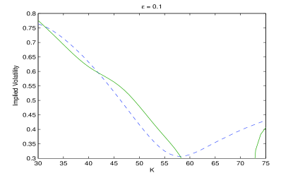
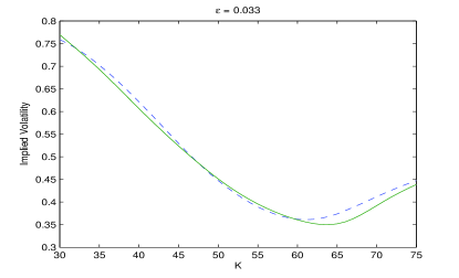
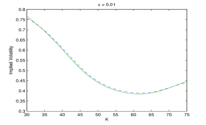
Figure 1: Using the model described in section 4, we plot the implied volatility induced by the price of European call option as a function of the strike price $K$. In each plot, the dashed blue line corresponds to the implied volatility induced by the full price $u^{\varepsilon}$ (computed via Monte Carlo simulation) and the solid green line corresponds to the implied volatility induced by our approximation $u_{0}+\varepsilon u_{1}$. For all plots we use the following parameter values: $t=1/10$, $e^{x}=50$, $m=-0.2$, $s=0.2$, $\rho=-0.7$, $a=0.2$, $b=1.5$, $\beta=1.0$ and $\Lambda=0.25$.

5 Calibration to S&P500 index options

In this section we calibrate ExtMerton jump-diffusion class discussed in Section 4 to the implied volatility surface of S&P500 options. For comparison, we also calibrate the classical Merton model and the fast mean-reverting stochastic volatility (FMR-SV) class of models of Fouque, Papanicolaou, and Sircar (2000) to the same set of data.

In order to formulate the calibration procedure, we introduce the following notation

$$\theta :=(\langle\sigma^{2}\rangle,\langle\zeta\rangle,m,s,V_{2}^{\varepsilon},V_{3}^{\varepsilon},U_{2}^{\varepsilon},U_{3}^{\varepsilon}),$$ (5.1)

$$\Theta :=\{\theta:\langle\sigma^{2}\rangle>0,\langle\zeta\rangle\geq 0,m\in\mathbb{R},s\geq 0,(V_{2}^{\varepsilon},V_{3}^{\varepsilon},U_{2}^{\varepsilon},U_{3}^{\varepsilon})\in\mathbb{R}^{4}\},$$ (5.2)

where we have defined $V_{i}^{\varepsilon}:=\varepsilon\,V_{i}$ and $U_{i}^{\varepsilon}:=\varepsilon\,U_{i}$. Note that the components of $\theta$ are the unobservable parameters needed to compute the approximate price of an option $u_{0}+\varepsilon\,u_{1}$ in the ExtMerton framework, and $\Theta$ is the feasible state space of these parameters. Note also that we do not assume a specific value for $\varepsilon$, a specific volatility process $Y$, or specific functions: $\sigma(y)$ or $\zeta(y)$. In fact, this is one of the main features of the class of models considered in this paper. By assuming that the driving factor $Y$ is fast-varying and ergodic, specific choices for ($\varepsilon$, $Y$, $\sigma(y)$, $\zeta(y)$) are not needed to compute the approximate price $u_{0}+\varepsilon\,u_{1}$ of an option (or the corresponding implied volatility). For the purposes of calibration and pricing, the relevant information about ($\varepsilon$, $Y$, $\sigma(y)$, $\zeta(y)$) is neatly contained in $\langle\sigma^{2}\rangle$, $\langle\zeta\rangle$ and the four group parameters $\{V_{i}^{\varepsilon},U_{i}^{\varepsilon},i=1,2\}$.

Let $I^{\text{obs}}(t,k)$ be the observed implied volatility of a European call option with time to maturity $t$ and $\log$ strike $k=\log K$. Let $I^{\varepsilon}(t,k;\theta)$ be the implied volatility of a European call option with the same maturity and strike as computed in the ExtMerton framework using parameters $\theta\in\Theta$. We formulate the calibration problem for the ExtMerton class as a least squares optimization. That is, we seek $\theta^{*}$ such that

$$\min_{\theta\in\Theta}\sum_{i}\left(I^{\text{obs}}(t_{i},k_{i})-I^{\varepsilon}(t_{i},k_{i};\theta)\right)^{2} =\sum_{i}\left(I(t_{i},k_{i})-I^{\varepsilon}(t_{i},k_{j};\theta^{*})\right)^{2}.$$ (5.3)

Here, the sum runs over all pairs $(t_{i},k_{i})$ in the data set. Note: we do not calibrate maturity-by-maturity. The calibration procedures for the Merton model and the FMR-SV class are performed in a similar fashion by solving (5.3) for $\theta\in\Theta^{\text{Mer}}$ and $\theta\in\Theta^{\text{FMR}}$ respectively, where

$$\Theta^{\textrm{Mer}} :=\{\theta:\langle\sigma^{2}\rangle>0,\langle\zeta\rangle\geq 0,m\in\mathbb{R},s\geq 0,(V_{2}^{\varepsilon},V_{3}^{\varepsilon},U_{2}^{\varepsilon},U_{3}^{\varepsilon})=0\},$$ (5.4)

$$\Theta^{\textrm{FMR}} :=\{\theta:\langle\sigma^{2}\rangle>0,(\langle\zeta\rangle,m,s)=0,(V_{2}^{\varepsilon},V_{3}^{\varepsilon})\in\mathbb{R}^{2},(U_{2}^{\varepsilon},U_{3}^{\varepsilon})=0\}.$$ (5.5)

Note that by requiring $(V_{2}^{\varepsilon},V_{3}^{\varepsilon},U_{2}^{\varepsilon},U_{3}^{\varepsilon})=0$ in $\Theta^{\text{Mer}}$ the effects of stochastic volatility and stochastic jump intensity disappear, and the approximate option price in the ExtMerton class $u_{0}+\varepsilon\,u_{1}$ reduces to the Merton price $u_{0}$. Similarly, by requiring that $(\langle\zeta\rangle,m,s,U_{2}^{\varepsilon},U_{3}^{\varepsilon})=0$ in $\Theta^{\text{FMR}}$, the effect of the jumps disappears (the effects of stochastic volatility remain), and the approximate option price in the ExtMerton class $u_{0}+\varepsilon\,u_{1}$ reduces to the price as computed in the FMR-SV class.

We perform the calibration procedure for all three frameworks (ExtMerton class, classical Merton model, and FMR-SV class) on S&P500 index options on four separate dates:

• January 4, 2010 encompassing maturities of 47, 75 and 103 days,

• October 1, 2010 encompassing maturities of 50, 78 and 113 days,

• December 19, 2011 encompassing maturities of 59, 88, 122, 177, 273 and 363 days, and

• January 11, 2012 encompassing maturities of 66, 100, 155, 251 and 341 days.

To perform the calibration we use Matlab’s built-in non-linear least squares optimizer: fmincon. The obtained fits for all three models are plotted in Figures 2, 3, 4 and 5. For each plot, the units of the horizontal axis are log-moneyness: $\text{LM}:=k-x$. The vertical axis represents implied volatility. Summarizing statistics can be found in Table Exponential Lévy-type models with stochastic volatility and jump intensity.

A visual inspection of figures 2, 3, 4 and 5 clearly supports the use of the ExtMerton class over both the Merton model and the FMR-SV class. The visual evidence is confirmed by the obtained root mean-square error (RMSE), which for the ExtMerton class is of the same order as the implied volatility bid-ask spread. Furthermore, the ExtMerton RMSE is less than half the RMSE of the classical Merton model and roughly one fourth the RMSE of the FMR-SV class. Intuitively, the reason for the improved fit in ExtMerton class is that to obtain a tight fit at longer maturities one requires a model with stochastic volatility, whereas short maturities require a model with jumps in order to reproduce the strong smile.

To further support the addition of stochastic volatility and jump intensity we consider other Lévy measures: Gumbel, Variance Gamma, uniform and Dirac. For each measure we calibrate the corresponding Lévy model and its extended counterpart to S&P500 implied volatilities from December 19, 2011. As in the Merton model, we observe that the RMSE for the extended models is of the order of the implied volatility bid-ask spread and roughly one half the RMSE of the classical Lévy counterparts. Summarizing statistics can be found in table Exponential Lévy-type models with stochastic volatility and jump intensity.

Extended Merton	Merton	FMR-SV
47 days-to-maturity	47 days-to-maturity	47 days-to-maturity
75 days-to-maturity	75 days-to-maturity	75 days-to-maturity
103 days-to-maturity	103 days-to-maturity	103 days-to-maturity

Figure 2: Implied volatility fit to S&P500 index options from January 4, 2010.

Extended Merton	Merton	FMR-SV
50 days-to-maturity	50 days-to-maturity	50 days-to-maturity
78 days-to-maturity	78 days-to-maturity	78 days-to-maturity
113 days-to-maturity	113 days-to-maturity	113 days-to-maturity

Figure 3: Implied volatility fit to S&P500 index options from October 1, 2010.

Extended Merton	Merton	FMR-SV
59 days-to-maturity	59 days-to-maturity	59 days-to-maturity
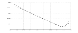
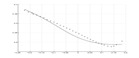
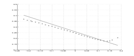
88 days-to-maturity	88 days-to-maturity	88 days-to-maturity
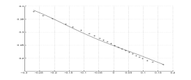
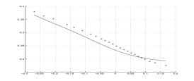
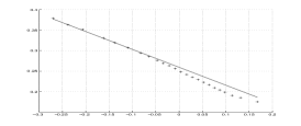
122 days-to-maturity	122 days-to-maturity	122 days-to-maturity
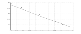
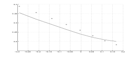
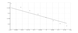
177 days-to-maturity	177 days-to-maturity	177 days-to-maturity
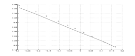
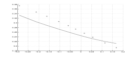
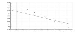
273 days-to-maturity	273 days-to-maturity	273 days-to-maturity
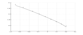
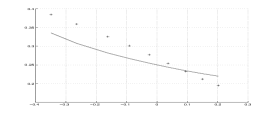
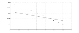
363 days-to-maturity	363 days-to-maturity	363 days-to-maturity

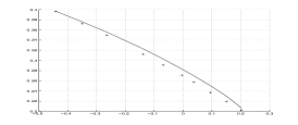
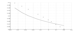
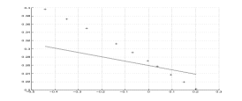
Figure 4: Implied volatility fit to S&P500 index options from December 19, 2011.

Extended Merton	Merton	FMR-SV
66 days-to-maturity	66 days-to-maturity	66 days-to-maturity
100 days-to-maturity	100 days-to-maturity	100 days-to-maturity
155 days-to-maturity	155 days-to-maturity	155 days-to-maturity
251 days-to-maturity	251 days-to-maturity	251 days-to-maturity
341 days-to-maturity	341 days-to-maturity	341 days-to-maturity

Figure 5: Implied volatility fit to S&P500 index options from January 11, 2012.

6 Extension to multiscale stochastic volatility and jump intensity

The results of this paper can be extended in a straightforward manner to include multiscale stochastic volatility and jump intensity. We briefly describe how this may be done. Our intent in this section is not to be rigorous, but rather to give a flavor of the computations involved in this extension. To begin, we modify the dynamics of $S$ slightly. Letting $S=e^{X}$ we have

$$\left.\begin{aligned} dX_{t}&=\gamma(Y_{t},Z_{t})\,dt+\sigma(Y_{t},Z_{t})\,d\widetilde{W}_{t}^{x}+\int_{\mathbb{R}}s\,d\widetilde{N}_{t}(Y_{t},Z_{t},ds),&X_{0}&=x,\\ dY_{t}&=\left(\frac{1}{\varepsilon^{2}}\alpha(Y_{t})-\frac{1}{\varepsilon}\Lambda(Y_{t},Z_{t})\,\beta(Y_{t})\right)dt+\frac{1}{\varepsilon}\beta(Y_{t})d\widetilde{W}_{t}^{y},&Y_{0}&=y,\\ dZ_{t}&=\Big{(}\delta^{2}c(Z_{t})-\delta\,\Gamma(Y_{t},Z_{t})\,g(Z_{t})\Big{)}dt+\delta\,g(Z_{t})d\widetilde{W}_{t}^{z},&Z_{0}&=z.\end{aligned}\right\}\qquad(\text{under $\widetilde{\mathbb{P}}$})$$ (6.1)

Here, $Z$ is a slow-varying factor, in the sense that its infinitesimal generator under $\mathbb{P}$ is scaled by $\delta^{2}$, which is assumed to be a small parameter: $\delta^{2}<<1$. The Brownian motions $\widetilde{W}^{x}$, $\widetilde{W}^{y}$, $\widetilde{W}^{z}$ have correlations $\rho_{xy}$, $\rho_{xz}$ and $\rho_{yz}$ (which must be such that the covariance matrix is positive definite), the compensated Poisson random measure $\widetilde{N}(Y,Z,ds)$ satisfies

$$d\widetilde{N}_{t}(Y_{t},Z_{t},ds) =dN_{t}(Y_{t},Z_{t},ds)-\zeta(Y_{t},Z_{t})\nu(ds)dt,$$ (6.2)

$$\widetilde{\mathbb{E}}[dN_{t}(Y_{t},Z_{t},ds)|Y_{t},Z_{t}] =\zeta(Y_{t},Z_{t})\nu(ds)dt,$$ (6.3)

and the drift $\gamma(Y_{t},Z_{t})$ is given by

$$\gamma(Y_{t},Z_{t}) =-\frac{1}{2}\sigma^{2}(Y_{t},Z_{t})-\zeta(Y_{t},Z_{t})\int_{\mathbb{R}}(e^{s}-1-s)\nu(ds).$$ (6.4)

Using risk-neutral pricing, the value $u^{\varepsilon,\delta}(t,x,y,z)$ of a European option in this setting is

$$u^{\varepsilon,\delta}(t,x,y,z) =\widetilde{\mathbb{E}}_{x,y,z}\left[h(X_{t})\right], h(x) :=H(e^{x}).$$ (6.5)

From the Kolmogorov backward equation, the function $u^{\varepsilon,\delta}$ satisfies the following PIDE and BC

$$\left(-\partial_{t}+\mathscr{A}^{\varepsilon,\delta}\right)u^{\varepsilon,\delta} =0, u^{\varepsilon,\delta}(0,x,y,z) =h(x),$$ (6.6)

where the partial integro-differential operator $\mathscr{A}^{\varepsilon,\delta}$ is the generator of $(X,Y,Z)$. The operator $\mathscr{A}^{\varepsilon,\delta}$ has the following form

$$\mathscr{A}^{\varepsilon,\delta} =\frac{1}{\varepsilon^{2}}\mathscr{A}_{0}+\frac{1}{\varepsilon}\mathscr{A}_{1}+\mathscr{A}_{2}+\frac{\delta}{\varepsilon}\mathscr{M}_{3}+\delta\,\mathscr{M}_{1}+\delta^{2}\,\mathscr{M}_{2}.$$ (6.7)

Terms containing $\delta$ in (6.6) are small in the small-$\delta$ limit, giving rise to a regular perturbation. Thus, (6.6) has the form of a combined singular-regular perturbation about the $\mathscr{O}(1)$ operator $(-\partial_{t}+\mathscr{A}_{2})$. Following Fouque et al. (2011) we seek a solution $u^{\varepsilon,\delta}$ of the form

$$u^{\varepsilon,\delta} =\sum_{n=0}^{\infty}\sum_{m=0}^{\infty}\varepsilon^{n}\delta^{m}u_{n,m}.$$ (6.8)

Our goal is to find an approximation $u^{\varepsilon,\delta}=u_{0,0}+\varepsilon\,u_{1,0}+\delta\,u_{0,1}+\mathscr{O}(\varepsilon^{2}+\delta^{2})$. A formal asymptotic analysis yields the following PIDEs for $u_{0,0}$, $u_{1,0}$ and $u_{0,1}$

$$\mathscr{O}(1): (-\partial_{t}+\langle\mathscr{A}_{2}\rangle)u_{0,0} =0, u_{0,0}(0,x,z) =h(x),$$ (6.9)

$$\mathscr{O}(\varepsilon): (-\partial_{t}+\langle\mathscr{A}_{2}\rangle)u_{1,0} =-\mathscr{B}u_{0,0}, u_{1,0}(0,x,z) =0,$$ (6.10)

$$\mathscr{O}(\delta): (-\partial_{t}+\langle\mathscr{A}_{2}\rangle)u_{0,1} =-\langle\mathscr{M}_{1}\rangle u_{0,0}, u_{0,1}(0,x,z) =0,$$ (6.11)

where, as in Section 3.1, the $y$-dependence has disappeared from $u_{0,0}$, $u_{1,0}$ and $u_{0,1}$. The operators $\langle\mathscr{A}_{2}\rangle$, $\mathscr{B}$ and $\langle\mathscr{M}_{1}\rangle$ are given by

$$\langle\mathscr{A}_{2}\rangle =\langle\gamma(\cdot,z)\rangle\partial_{x}+\frac{1}{2}\langle\sigma^{2}(\cdot,z)\rangle\partial_{xx}^{2}+\langle\zeta(\cdot,z)\rangle\int_{\mathbb{R}}\left(e^{s\partial_{x}}-1-s\partial_{x}\right)\nu(ds),$$ (6.12)

$$\mathscr{B} =V_{3}(z)\left(\partial_{xxx}^{3}-\partial_{xx}^{2}\right)+U_{3}(z)\left(-\int_{\mathbb{R}}\Big{(}e^{s}-1-s\Big{)}\nu(ds)\partial_{xx}^{2}+\int_{\mathbb{R}}\Big{(}\theta_{s}-1-s\partial_{x}\Big{)}\partial_{x}\nu(ds)\right)$$ (6.13)

$$\qquad+V_{2}(z)\left(\partial_{xx}^{2}-\partial_{x}\right)+U_{2}(z)\left(-\int_{\mathbb{R}}\Big{(}e^{s}-1-s\Big{)}\nu(ds)\partial_{x}+\int_{\mathbb{R}}\Big{(}\theta_{s}-1-s\partial_{x}\Big{)}\nu(ds)\right),$$ (6.14)

$$\langle\mathscr{M}_{1}\rangle =-g(z)\langle\Gamma(\cdot,z)\rangle\partial_{z}+g(z)\rho_{xz}\langle\sigma(\cdot,z)\rangle\partial_{xz}^{2},$$ (6.15)

where the $z$-dependent parameters ($V_{3}(z)$, $U_{3}(z)$, $V_{2}(z)$, $U_{2}(z)$) are

$$V_{3}(z) =-\frac{\rho_{xy}}{2}\langle\beta(\cdot)\sigma(\cdot,z)\partial_{y}\eta(\cdot,z)\rangle, U_{3}(z) =-\rho_{xy}\langle\beta(\cdot)\sigma(\cdot,z)\partial_{y}\xi(\cdot,z)\rangle,$$ (6.16)

$$V_{2}(z) =\frac{1}{2}\langle\beta(\cdot)\Lambda(\cdot,z)\partial_{y}\eta(\cdot,z)\rangle, U_{2}(z) =\langle\beta(\cdot)\Lambda(\cdot,z)\partial_{y}\xi(\cdot,z)\rangle.$$ (6.17)

The expressions for $u_{0,0}$ and $u_{1,0}$ are analogous to those given for $u_{0}$ and $u_{1}$ in Theorem 3.1. An expression for $u_{0,1}$ is obtained using Fourier transforms

$$\widehat{v}(s,\lambda,z) :=\int_{\mathbb{R}}dx\frac{1}{\sqrt{2\pi}}e^{-i\lambda x}\langle\mathscr{M}_{1}\rangle u_{0,0}(s,x,z)$$ (6.18)

$$u_{0,1}(t,x,z) =\int_{\mathbb{R}}d\lambda\,\frac{1}{\sqrt{2\pi}}e^{i\lambda x}\int_{0}^{t}ds\,e^{(t-s)\phi_{\lambda}(z)}\widehat{v}(s,\lambda,z).$$ (6.19)

Note, care must be taken when computing $\langle\mathscr{M}_{1}\rangle u_{0,0}$ as both terms in $\langle\mathscr{M}_{1}\rangle$ contain the operator $\partial_{z}$ and $u_{0,0}$ depends on $z$ through both $\langle\sigma^{2}(\cdot,z)\rangle$ and $\langle\zeta(\cdot,z)\rangle$. A careful computation shows that $u_{0,1}$ is linear in the following four parameters

$$V_{1}(z) =g(z)\rho_{xz}\langle\sigma(\cdot,z)\rangle\partial_{z}\langle\sigma^{2}(\cdot,z)\rangle, V_{0}(z) =-g(z)\langle\Gamma(\cdot,z)\rangle\partial_{z}\langle\sigma^{2}(\cdot,z)\rangle,$$ (6.20)

$$U_{1}(z) =g(z)\rho_{xz}\langle\sigma(\cdot,z)\rangle\partial_{z}\langle\zeta(\cdot,z)\rangle, U_{0}(z) =-g(z)\langle\Gamma(\cdot,z)\rangle\partial_{z}\langle\zeta(\cdot,z)\rangle.$$ (6.21)

From the arguments in Fouque et al. (2011), Chapter 4, it follows that for fixed $(t,x,y)$ there exists a constant $C$ such that $|u^{\varepsilon,\delta}-(u_{0,}+\varepsilon\,u_{1,0}+\delta\,u_{0,1})|<C(\varepsilon^{2}+\delta^{2})$ when $h$ is smooth.

7 Conclusion

In this paper, we have introduced a class of exponential Lévy-type models in which the volatility and jump-intensity are driven stochastically by two factors – one fast-varying and one slow-varying. Using techniques from the theory of generalized Fourier transforms, singular and regular perturbation theory we have derived a general formula for the approximate price of any European-style derivative whose payoff function has a generalized Fourier transform. We test five specific examples of exponential Lévy-type models with stochastic volatility and jump-intensity (the Extended Merton, Gumbel, Dirac, Variance Gamma, and Uniform) and we show that these model classes provide a closer fit to the S&P500 implied volatility surface than either the Merton model or the class of fast mean-reverting stochastic volatility models. Other exponential Lévy models can be extended in a similar fashion by choosing the appropriate Lévy measure $\nu$. We hope this work motivates further research into exponential Lévy-type models. A possible extension of this paper, for example, would be to allow the jump distribution (rather than just the jump intensity) to vary stochastically in time.

Acknowledgments

The author would like to extend his sincerest thanks to Ramon van Handel, Ronnie Sircar, Jean-Pierre Fouque, Rama Cont, Jose-Luis Menaldi and Erhan Bayraktar, whose comments and suggestions have improved the quality and readability of this manuscript.

Appendix A Proof the Theorem 3.1

We wish to solve PIDEs (3.16) and (3.23) with BCs (3.28) and (3.29) respectively. For simplicity, we solve these equations for a payoff $h\in L^{1}(\mathbb{R},dx)$. The results extend to any $h$ with a generalized Fourier transform in a straightforward manner.

To begin, we recall that the Fourier transform $\widehat{f}$ and inverse transform of a function $f\in L^{1}(\mathbb{R},dx)$ are defined as a pair

$$\text{Fourier Transform}: \widehat{f}(\lambda) :=\frac{1}{\sqrt{2\pi}}\int_{\mathbb{R}}dx\,e^{-i\lambda x}f(x), \lambda\in\mathbb{R},$$ (A.1)

$$\text{Inverse Transform}: f(x) =\frac{1}{\sqrt{2\pi}}\int d\lambda\,e^{i\lambda x}\widehat{f}(\lambda).$$ (A.2)

Next, we introduce $\langle\mathscr{A}_{2}\rangle^{*}$, the formal adjoint of $\langle\mathscr{A}_{2}\rangle$, which satisfies

$$\int_{\mathbb{R}}dx\,e^{-i\lambda x}\langle\mathscr{A}_{2}\rangle f(x)dx =\int_{\mathbb{R}}dx\,f(x)\langle\mathscr{A}_{2}\rangle^{*}e^{-i\lambda x}dx.$$ (A.3)

The operator $\langle\mathscr{A}_{2}\rangle^{*}$ can be obtained through by integration by parts, which leads to

$$\langle\mathscr{A}_{2}\rangle^{*} =-\langle\gamma\rangle\partial_{x}+\frac{1}{2}\langle\sigma^{2}\rangle\partial_{xx}^{2}+\langle\zeta\rangle\int_{\mathbb{R}}\left(\theta_{-z}-1+z\partial_{x}\right)\nu(dz).$$ (A.4)

We note that

$$\langle\mathscr{A}_{2}\rangle^{*}e^{-i\lambda x} =\phi_{\lambda}e^{-i\lambda x}, \mathscr{B}e^{i\lambda x} =B_{\lambda}e^{i\lambda x},$$ (A.5)

where $\phi_{\lambda}$ and $B_{\lambda}$ are given by (3.33) and (3.35) respectively. To find an expression for $u_{0}(t,x)$ we Fourier transform PIDE (3.16) and BC (3.28). We have,

$$\partial_{t}u_{0}(t,x) =\langle\mathscr{A}_{2}\rangle u_{0}(t,x) \Rightarrow \frac{1}{\sqrt{2\pi}}\int_{\mathbb{R}}dx\,e^{-i\lambda x}\partial_{t}u_{0}(t,x) =\frac{1}{\sqrt{2\pi}}\int_{\mathbb{R}}dx\,e^{-i\lambda x}\langle\mathscr{A}_{2}\rangle u_{0}(t,x)$$ (A.6)

$$=\frac{1}{\sqrt{2\pi}}\int_{\mathbb{R}}dx\,u_{0}(t,x)\langle\mathscr{A}_{2}\rangle^{*}e^{-i\lambda x}$$ (A.7)

$$=\phi_{\lambda}\frac{1}{\sqrt{2\pi}}\int_{\mathbb{R}}dx\,u_{0}(t,x)e^{-i\lambda x}$$ (A.8)

$$\Rightarrow \partial_{t}\widehat{u}_{0}(t,\lambda) =\phi_{\lambda}\widehat{u}_{0}(t,\lambda),$$ (A.9)

$$u_{0}(0,x) =h(x) \Rightarrow \widehat{u}_{0}(0,\lambda) =\widehat{h}(\lambda).$$ (A.10)

Note that (A.9) is an ODE in $t$ for $\widehat{u}_{0}(t,\lambda)$ with an initial condition (A.10). Thus, one deduces

$$\widehat{u}_{0}(t,\lambda) =e^{t\phi_{\lambda}}\widehat{h}(\lambda) \Rightarrow u_{0}(t,x) =\frac{1}{\sqrt{2\pi}}\int_{\mathbb{R}}d\lambda e^{t\phi_{\lambda}}\widehat{h}(\lambda)e^{i\lambda x},$$ (A.11)

which established (3.36). Next, to find an expression for $u_{1}(t,x)$ we first observe that

$$\mathscr{B}u_{0}(t,x) =\frac{1}{\sqrt{2\pi}}\int_{\mathbb{R}}d\mu\,e^{t\phi_{\mu}}\widehat{h}(\mu)\mathscr{B}e^{i\mu x}=\frac{1}{\sqrt{2\pi}}\int_{\mathbb{R}}d\mu\,e^{t\phi_{\mu}}\widehat{h}(\mu)B_{\mu}e^{i\mu x}.$$ (A.12)

Therefore, we have

$$\frac{1}{\sqrt{2\pi}}\int_{\mathbb{R}}dx\,e^{-i\lambda x}\mathscr{B}u_{0}(t,x) =\int_{\mathbb{R}}d\mu\,e^{t\phi_{\mu}}\widehat{h}(\mu)B_{\mu}\frac{1}{2\pi}\int_{\mathbb{R}}dx\,e^{-i(\lambda-\mu)x}$$ (A.13)

$$=\int_{\mathbb{R}}d\mu\,e^{t\phi_{\mu}}\widehat{h}(\mu)B_{\mu}\delta(\mu-\lambda)$$ (A.14)

$$=e^{t\phi_{\lambda}}\widehat{h}(\lambda)B_{\lambda},$$ (A.15)

where we have used the Fourier representation of a Dirac delta function: $\frac{1}{2\pi}\int_{\mathbb{R}}dx\,e^{-i(\lambda-\mu)x}=\delta(\lambda-\mu)$. Fourier Transforming PIDE (3.23) and BC (3.29) one finds

$$(-\partial_{t}+\phi_{\lambda})\widehat{u}_{1}(t,\lambda) =-e^{t\phi_{\lambda}}\widehat{h}(\lambda)B_{\lambda} \widehat{u}_{1}(0,\lambda) =0.$$ and (A.16)

Once again, have an (inhomogeneous) ODE in $t$ for $\widehat{u}_{1}(t,\lambda)$. Solving the ODE explicitly for $\widehat{u}_{1}(t,\lambda)$ and inverse transforming from $\lambda$ to $x$ yields.

$$\widehat{u}_{1}(t,\lambda) =te^{t\phi_{\lambda}}\widehat{h}(\lambda)B_{\lambda} \Rightarrow u_{1}(t,x) =\frac{1}{\sqrt{2\pi}}\int_{\mathbb{R}}d\lambda\,te^{t\phi_{\lambda}}\widehat{h}(\lambda)B_{\lambda}e^{i\lambda x},$$ (A.17)

which establishes (3.37). This completes the proof.

Table 1: Calibration results for January 4, 2010, October 1, 2010 and January 11, 2012. The first date encompasses the following maturities: 47, 75, and 103 days. The second date contains the maturities 50, 78 and 113 days. The third contains the maturities 66, 10, 155, 251, 341 days.

2010/01/04									DTM:47-103
FMRSV	$\langle\sigma^{2}\rangle$				$V_{3}$		$V_{2}$		RMSE
	$0.1981^{2}$				$-7\cdot 10^{-4}$		$10^{-5}$		0.0189
Merton	$\langle\sigma^{2}\rangle$	$\langle\zeta\rangle$	$m$	$s^{2}$					RMSE
$\nu(dz)=(2\pi s^{2})^{-1/2}\exp\left(-\frac{(z-m)^{2}}{2s^{2}}\right)$	$0.1409^{2}$	0.1708	$-$0.1708	$0.1371^{2}$					0.0144
ExtendedMerton	$\langle\sigma^{2}\rangle$	$\langle\zeta\rangle$	$m$	$s^{2}$	$V_{3}^{\varepsilon}$	$U_{3}^{\varepsilon}$	$V_{2}^{\varepsilon}$	$U_{2}^{\varepsilon}$	RMSE
$\nu(dz)=(2\pi s^{2})^{-1/2}\exp\left(-\frac{(z-m)^{2}}{2s^{2}}\right)$	$0.1346^{2}$	0.653	$-$0.208	$0.1729^{2}$	$-2\cdot 10^{-5}$	0.0072	0.001	$-$0.0058	0.0049
2010/10/01									DTM: 50-113
FMRSV	$\langle\sigma^{2}\rangle$				$V_{3}$		$V_{2}$		RMSE
	$0.2222^{2}$				$-0.0011$		$10^{-5}$		0.0222
Merton	$\langle\sigma^{2}\rangle$	$\langle\zeta\rangle$	$m$	$s^{2}$					RMSE
$\nu(dz)=(2\pi s^{2})^{-1/2}\exp\left(-\frac{(z-m)^{2}}{2s^{2}}\right)$	$0.1538^{2}$	0.6617	$-$0.1895	$0.1525^{2}$					0.0183
ExtendedMerton	$\langle\sigma^{2}\rangle$	$\langle\zeta\rangle$	$m$	$s^{2}$	$V_{3}^{\varepsilon}$	$U_{3}^{\varepsilon}$	$V_{2}^{\varepsilon}$	$U_{2}^{\varepsilon}$	RMSE
$\nu(dz)=(2\pi s^{2})^{-1/2}\exp\left(-\frac{(z-m)^{2}}{2s^{2}}\right)$	$0.1437^{2}$	0.5187	$-$0.295	$0.2159^{2}$	$-3\cdot 10^{-5}$	0.0132	$-$0.0027	0.0142	0.0052
2012/01/11									DTM:66-341
FMRSV	$\langle\sigma^{2}\rangle$				$V_{3}$		$V_{2}$		RMSE
	$0.35^{2}$				$0.0049$		$0.0513$		0.0373
Merton	$\langle\sigma^{2}\rangle$	$\langle\zeta\rangle$	$m$	$s^{2}$					RMSE
$\nu(dz)=(2\pi s^{2})^{-1/2}\exp\left(-\frac{(z-m)^{2}}{2s^{2}}\right)$	$0.1422^{2}$	0.2319	$-0.2858$	$0.1705^{2}$					0.0298
ExtendedMerton	$\langle\sigma^{2}\rangle$	$\langle\zeta\rangle$	$m$	$s^{2}$	$V_{3}^{\varepsilon}$	$U_{3}^{\varepsilon}$	$V_{2}^{\varepsilon}$	$U_{2}^{\varepsilon}$	RMSE
$\nu(dz)=(2\pi s^{2})^{-1/2}\exp\left(-\frac{(z-m)^{2}}{2s^{2}}\right)$	$0.1073^{2}$	0.7606	$-0.1988$	$0.1543^{2}$	$-6.0052\cdot 10^{-5}$	0.0010	$6.8192\cdot 10^{-4}$	$-3.045\cdot 10^{-4}$	0.0125

Table 2: Calibration results for December 19, 2011. The dataset contains the following maturities: 59, 88, 122, 177, 273 and 363 days.

2011/12/19										DTM:59-363
FMRSV	$\langle\sigma^{2}\rangle$					$V_{3}$		$V_{2}$		RMSE
	$0.35^{2}$					$0.004811$		$0.03717$		0.0278
Merton	$\langle\sigma^{2}\rangle$	$\langle\zeta\rangle$	$m$	$s^{2}$						RMSE
$\nu(dz)=(2\pi s^{2})^{-1/2}\exp\left(-\frac{(z-m)^{2}}{2s^{2}}\right)$	$0.1529^{2}$	1.3720	$-$0.1397	$0.1141^{2}$						0.0215
ExtendedMerton	$\langle\sigma^{2}\rangle$	$\langle\zeta\rangle$	$m$	$s^{2}$		$V_{3}^{\varepsilon}$	$U_{3}^{\varepsilon}$	$V_{2}^{\varepsilon}$	$U_{2}^{\varepsilon}$	RMSE
$\nu(dz)=(2\pi s^{2})^{-1/2}\exp\left(-\frac{(z-m)^{2}}{2s^{2}}\right)$	$0.2054^{2}$	0.8207	$-$0.5608	$0.4070^{2}$		$-5.61729\cdot 10^{-4}$	0.3254	$-$0.1263	$-$0.1549	0.0072
Gumbel	$\langle\sigma^{2}\rangle$	$\langle\zeta\rangle$	$m$	$s^{2}$						RMSE
$\nu(dz)=\frac{1}{\sigma}\exp\left(\left(\frac{x-m}{\sigma}\right)-\exp\left(\frac{x-m}{\sigma}\right)\right)$	$0.0705^{2}$	5.3221	$-$0.1875	$0.0756^{2}$						0.0202
ExtendedGumbel	$\langle\sigma^{2}\rangle$	$\langle\zeta\rangle$	$m$	$s^{2}$		$V_{3}^{\varepsilon}$	$U_{3}^{\varepsilon}$	$V_{2}^{\varepsilon}$	$U_{2}^{\varepsilon}$	RMSE
$\nu(dz)=\frac{1}{\sigma}\exp\left(\left(\frac{x-m}{\sigma}\right)-\exp\left(\frac{x-m}{\sigma}\right)\right)$	$0.0717^{2}$	6.2521	$-$0.1875	$0.0856^{2}$		$-1.2232\cdot 10^{-5}$	$-$4.1826$\cdot 10^{-6}$	6.6619$\cdot 10^{-5}$	1.3969$\cdot 10^{-6}$	0.0116
Dirac	$\langle\sigma^{2}\rangle$	$\langle\zeta\rangle$	$a$							RMSE
$\nu(dz)=\delta_{a}(dz)$	$0.1418^{2}$	1.5924	$-$0.1810							0.0212
ExtendedDirac	$\langle\sigma^{2}\rangle$	$\langle\zeta\rangle$	$a$			$V_{3}^{\varepsilon}$	$U_{3}^{\varepsilon}$	$V_{2}^{\varepsilon}$	$U_{2}^{\varepsilon}$	RMSE
$\nu(dz)=\delta_{a}(dz)$	$0.1398^{2}$	1.3523	$-$0.1768			$-2.7651\cdot 10^{-5}$	1.2326$\cdot 10^{-5}$	4.5501$\cdot 10^{-5}$	1.8360$\cdot 10^{-5}$	0.0123
Variance Gamma	$\langle\sigma^{2}\rangle$	$\langle\zeta\rangle$	$a$	$b$	$B$					RMSE
$\nu(dz)=\frac{e^{-az}}{z}\mathbf{1}\{z>0\}+B\frac{e^{bz}}{-z}\mathbf{1}\{z<0\}$	$0.0510^{2}$	0.6783	35.3325	11.4922	13.6786					0.0215
Extended Variance Gamma	$\langle\sigma^{2}\rangle$	$\langle\zeta\rangle$	$a$	$b$	$B$	$V_{3}^{\varepsilon}$	$U_{3}^{\varepsilon}$	$V_{2}^{\varepsilon}$	$U_{2}^{\varepsilon}$	RMSE
$\nu(dz)=\frac{e^{-az}}{z}\mathbf{1}\{z>0\}+B\frac{e^{bz}}{-z}\mathbf{1}\{z<0\}$	$0.0922^{2}$	0.1196	267.4499	14.8657	69.8231	$3\cdot 10^{-3}$	$-$0.0066	0.0011	$-7\cdot 10^{-4}$	0.0147
Uniform	$\langle\sigma^{2}\rangle$	$\langle\zeta\rangle$	$a$	$b$						RMSE
$\nu(dz)=\frac{1}{b-a}\mathbf{1}\{a\leq x\leq b\}$	$0.0922^{2}$	3.9644	$-$0.2086	0.0588						0.0214
ExtendedUniform	$\langle\sigma^{2}\rangle$	$\langle\zeta\rangle$	$a$			$V_{3}^{\varepsilon}$	$U_{3}^{\varepsilon}$	$V_{2}^{\varepsilon}$	$U_{2}^{\varepsilon}$	RMSE
$\nu(dz)=\frac{1}{b-a}\mathbf{1}\{a\leq x\leq b\}$	$0.1405^{2}$	4.0001	$-$0.1009	0.0997		$-4.74943\cdot 10^{-4}$	$1.1575\cdot 10^{-5}$	0.0078	$-5.3749\cdot 10^{-4}$	0.0142

References

- Black and Scholes (1973) Black, F. and M. Scholes (1973). The pricing of options and corporate liabilities. The journal of political economy 81(3), 637–654.
- Boyarchenko and Levendorskii (2002) Boyarchenko, S. and S. Levendorskii (2002). Non-Gaussian Merton-Black-Scholes Theory. World Scientific.
- Boyarchenko and Levendorskii (2000) Boyarchenko, S. I. and S. Z. Levendorskii (2000). Option pricing for truncated lévy processes. International Journal of Theoretical and Applied Finance 03(03), 549–552.
- Carr and Wu (2004) Carr, P. and L. Wu (2004). Time-changed Lévy processes and option pricing. Journal of Financial Economics 71(1), 113–141.
- Christoffersen et al. (2009) Christoffersen, P., K. Jacobs, and Ornthanalai (2009). Exploring Time-Varying Jump Intensities: Evidence from S&P500 Returns and Options. CIRANO.
- Cont and Tankov (2004) Cont, R. and P. Tankov (2004). Financial modelling with jump processes, Volume 2. Chapman & Hall.
- Eraker (2004) Eraker, B. (2004). Do stock prices and volatility jump? reconciling evidence from spot and option prices. The Journal of Finance 59(3), 1367–1404.
- Fouque et al. (2000) Fouque, J.-P., G. Papanicolaou, and R. Sircar (2000). Derivatives in Financial Markets with Stochastic Volatility. Cambridge University Press.
- Fouque et al. (2011) Fouque, J.-P., G. Papanicolaou, R. Sircar, and K. Solna (2011). Multiscale Stochastic Volatility for Equity, Interest-Rate and Credit Derivatives. Cambridge University Press.
- Kou (2002) Kou, S. (2002). A jump-diffusion model for option pricing. Management Science 48(8), 1086–1101.
- Lewis (2001) Lewis, A. (2001). A simple option formula for general jump-diffusion and other exponential Lévy processes.
- Lipton (2002) Lipton, A. (2002). The vol smile problem. Risk (February), 61–65.
- Madan et al. (1998) Madan, D., P. Carr, and E. Chang (1998). The variance gamma process and option pricing. European Finance Review 2(1), 79–105.
- Mandelbrot (1963) Mandelbrot, B. (1963). The variation of certain speculative prices. The journal of business 36(4), 394–419.
- Merton (1976) Merton, R. (1976). Option pricing when underlying stock returns are discontinuous. Journal of financial economics 3(1), 125–144.
- Øksendal and Sulem (2005) Øksendal, B. and A. Sulem (2005). Applied stochastic control of jump diffusions. Springer Verlag.