Non-Markovian qubit decoherence during dispersive readout

Abstract

We study qubit decoherence under generalized dispersive readout, i.e., we investigate a qubit coupled to a resonantly driven dissipative harmonic oscillator. We provide a complete picture by allowing for arbitrarily large qubit-oscillator detuning and by considering also a coupling to the square of the oscillator coordinate, which is relevant for flux qubits. Analytical results for the decoherence time are obtained by a transformation of the qubit-oscillator Hamiltonian to the dispersive frame and a subsequent master equation treatment beyond the Markov limit. We predict a crossover from Markovian decay to a decay with Gaussian shape. Our results are corroborated by the numerical solution of the full qubit-oscillator master equation in the original frame.

I Introduction

The final readout of the qubit state presents an essential part of any quantum algorithm Nielsen2000a . For solid state qubits, it is typically realized by coupling the qubit to a harmonic oscillator such that the oscillator frequency undergoes a shift whose sign depends on the state of the qubit. This shift can be probed by driving the oscillator at its bare frequency, with the consequence that the phase of the response provides information about the qubit state Chiorescu2004a ; Wallraff2004a ; Grajcar2004a ; Sillanpaa2005a ; Lupascu2006a ; Schuster2007a . Typically, one works with a qubit-oscillator detuning that is slightly larger than the respective mutual coupling while still being much smaller than the qubit splitting Chiorescu2004a ; Wallraff2004a . Then the resulting frequency shift of the oscillator can be derived from the Rabi Hamiltonian via a transformation to the so-called dispersive frame Blais2004a . For even stronger detuning, the transformation becomes more involved, but nevertheless the sign of the dispersive shift depends on the qubit state Zueco2009b and, thus, qubit readout remains possible. For an extreme detuning, such that the oscillator frequency exceeds the qubit splitting by far, a measurement protocol has been proposed by which one can reconstruct information about coherent qubit oscillations from recorded data Reuther2011b . Even though similar readout is possible by driving the qubit directly Reuther2009a ; Reuther2011a , the oscillator plays a constructive role as band pass.

For driving the oscillator and for measuring its response, the setup must be coupled to auxiliary electronic circuitry, which represents an environment that eventually destroys the phase of the qubit. Generally information about the qubit state can be obtained only at the rate at which the qubit coherence decays Clerk2010a . Thus a quantitative understanding of qubit decoherence stemming from the coupling to a resonantly driven oscillator is inevitable for the design of dispersive readout schemes. For sufficiently small detuning, such that the rotating-wave approximation underlying the Rabi Hamiltonian holds, the decoherence rate follows from an intuitive consideration in which the shot noise of the cavity photons randomizes the qubit phase Blais2004a . This result will emerge as limiting case of our more general picture.

For weakly dissipative quantum systems, Bloch-Redfield theory Redfield1957a ; Blum1996a represents a natural framework for studying decoherence, in particular when memory effects are minor. When qubit decoherence stems from a dissipative harmonic oscillator, however, its naive application may significantly overestimate the decoherence rate Thorwart2004a ; Nesi2007a because peaks in the effective spectral density of the oscillator Garg1985a ; Tian2002a ; vanderWal2003a cause non-Markovian behavior. This may in particular be the case for the ultra-strong qubit-oscillator coupling which marks a recent trend Devoret2007a ; Anappara2009a ; Ashhab2010a ; Niemczyk2010a .

Here we present a global picture of the qubit decoherence during dispersive readout. We consider both linear and quadratic qubit-oscillator coupling as well as arbitrarily large detuning, while we do not account for higher-order corrections to the dispersive shift Boissonneault2009a and non-linearities in the oscillator potential Boissonneault2012a . While in Ref. Tian2002a this problem was studied for an oscillator at thermal equilibrium, we focus on the semiclassical regime, in which the oscillator is governed by the driving. In Sec. II, we introduce our quantum master equation for the full qubit-oscillator-bath model. Section III is devoted to an analytical derivation of the dephasing time. We develop a picture in which the driven dissipative oscillator acts as a bath which is eliminated in second-order perturbation theory but beyond a Markov approximation. In order to corroborate the resulting dephasing time, we numerically solve in Sec. IV the quantum master equation for the qubit and the oscillator in the original frame.

II Qubit-oscillator model

The qubit coupled to the oscillator is described by the Hamiltonian

$$H_{0}=\frac{\hbar\epsilon}{2}\sigma_{z}+\hbar g_{1}\sigma_{x}(a^{\dagger}+a)+\hbar g_{2}\sigma_{x}(a^{\dagger}+a)^{2}+\hbar\omega_{0}a^{\dagger}a,$$ (1)

where $g_{1}$ is the strength of the dipole interaction which is linear in the oscillator displacement $a^{\dagger}+a$. The coupling to the square of the displacement with strength $g_{2}$ is mainly relevant for flux qubits and can be controlled to some extent Bertet2005a ; Bertet2005b .

The system state can be probed via a coupling an external circuitry which we model by the system-bath Hamiltonian

$$H_{\text{bath}}=(a^{\dagger}+a)\sum_{\nu}c_{\nu}(b_{\nu}^{\dagger}+b_{\nu})+\sum_{\nu}\hbar\omega_{\nu}b_{\nu}^{\dagger}b_{\nu},$$ (2)

where $b_{\nu}$ is the annihilation operator of a bath mode $\nu$. The influence of the bath is determined by the spectral density $I(\omega)=2\pi\sum_{\nu}c_{\nu}^{2}\delta(\omega-\omega_{\nu})$, which we assume to be ohmic, i.e., $I(\omega)=\gamma\omega/\omega_{0}$ with the oscillator damping rate $\gamma$.

An external ac driving corresponds to one particular bath mode being in a highly excited coherent state. It may be described as classical oscillation, such that the oscillator experiences a driving force $A\cos(\Omega t-\phi_{0})$. This corresponds to the driving Hamiltonian

$$H_{F}(t)=Ax\cos(\Omega t-\phi_{0}).$$ (3)

For convenience, we have introduced the dimensionless position and momentum operators $x=(a^{\dagger}+a)/\sqrt{2}$ and $p=i(a^{\dagger}-a)/\sqrt{2}$, respectively.

Within the usual Born-Markov approximation for the oscillator (see Appendix A), one obtains the master equation

$$\begin{split}\dot{R}=&-\frac{i}{\hbar}[H_{0}+H_{F}(t)]-\frac{i\gamma}{2}[x,[p,R]_{+}]\\ &-\frac{\gamma}{2}\coth\Big{(}\frac{\hbar\omega_{0}}{2k_{B}T}\Big{)}[x,[x,R]]\end{split}$$ (4)

for the joint density operator $R$ of the qubit and the oscillator. It provides all numerical results presented below. In case of low temperatures, $k_{B}T\ll\hbar\omega_{0}$, the hyperbolic cotangent assumes a value close to unity. Notice that in contrast to a parametric driving, the linearly coupled ac force does not affect the dissipative terms Kohler1997a . Moreover, we assume that the qubit couples only weakly to the oscillator, so that its influence on the dissipative kernel of the oscillator is negligible.

III Analytical estimate of the qubit dephasing time

Extracting from the master equation (4) an analytical expression for the qubit decoherence time represents a formidable task. Thus, we have to rely on several approximations that make use of the conditions under which dispersive readout may be performed. We start by a transformation to the dispersive frame which yields a coupling to the square of the position coordinate of the driven oscillator. The relevant influence on the qubit is determined by the corresponding auto correlation function which we evaluate in the semiclassical limit. It becomes stationary only after averaging within a rotating-wave approximation over the initial phase $\phi_{0}$ of the driving. Finally, the resulting non-Markovian master equation for the qubit is solved for short times.

III.1 Transformation to the dispersive frame

For the discussion of dispersive readout, the dispersive picture of the qubit-oscillator Hamiltonian $H_{0}$ has proven useful Blais2004a ; Clerk2010a ; Reuther2011b . In order to capture also very large qubit-oscillator detuning, we need to perform the according transformation beyond rotating-wave approximation. This yields the effective qubit-oscillator Hamiltonian Zueco2009b

$$\bar{H}_{0}=\frac{\hbar\epsilon}{2}\sigma_{z}+\hbar(\lambda_{\parallel}\sigma_{z}+\lambda_{\perp}\sigma_{x})x^{2}+\frac{\hbar\omega_{0}}{2}(x^{2}+p^{2})$$ (5)

with the coupling constants

$$\lambda_{\parallel}={} \frac{g_{1}^{2}}{\epsilon-\omega_{0}}+\frac{g_{1}^{2}}{\epsilon+\omega_{0}},$$ (6)

$$\lambda_{\perp}={} 2g_{2}.$$ (7)

Thus, the coupling linear in the oscillator coordinate has turned into a quadratic coupling with strength $\lambda_{\parallel}$, while $\lambda_{\perp}$ has been introduced for a unified notation. In correspondence to the orientation of the coupling operators on the Bloch sphere, we refer to the coupling terms as “longitudinal” and “transverse”, respectively.

If only energy-conserving terms in the qubit-oscillator coupling were considered Blais2004a , $\lambda_{\parallel}$ would be given by only the first term of Eq. (6) and, thus, be $\propto(\epsilon-\omega_{0})^{-1}$. By contrast, the second term of Eq. (6) turns the frequency dependence into $\lambda_{\parallel}\propto|\epsilon^{2}-\omega_{0}^{2}|^{-2}$. This means that for positive detuning, $\omega_{0}>\epsilon$, the counter-rotating terms diminish the dispersive shift. Since we will find that decoherence grows with $\lambda_{\parallel}$, the coherence time is larger than predicted within rotating-wave approximation Blais2004a .

The interpretation of the effective interaction is that it shifts the oscillator frequency by $\pm(\lambda_{\parallel}^{2}+\lambda_{\perp}^{2})^{1/2}$, where the sign depends on the state of the qubit. Therefore, probing the oscillator frequency provides information about the latter. In this work we are interested in the qubit decoherence that stems from this coupling. When transforming to the dispersive frame, the dissipative terms of the master equation (4) acquire a contribution from qubit operators Boissonneault2009b ; Reuther2010a , which, however, is negligible as compared to the terms considered below.

III.2 Driven oscillator as effective bath

We now treat the oscillator as environment coupled to the qubit coordinate $Y=\lambda_{\parallel}\sigma_{z}+\lambda_{\perp}\sigma_{x}$ via the Hamiltonian $\bar{H}_{\text{int}}=\hbar Y\eta$ with the environmental fluctuations $\eta$ determined by the operator $x^{2}$. Its expectation value $\langle x^{2}\rangle$ yields a correction to the qubit Hamiltonian of the order $\lambda_{\parallel}$. Therefore, the impact of $\langle x^{2}\rangle$ on the dissipative terms is already beyond the order considered herein and can be omitted, such that the relevant fluctuation reads

$$\eta=x^{2}-\langle x^{2}\rangle.$$ (8)

We assume weak dissipation such that the bath can be eliminated within second order perturbation theory. This is in accordance with our observation of predominantly coherent time evolution; see the numerical results in Sec. IV. Then the dissipative part of the master equation for the qubit density operator $\rho$ reads

$$\begin{split}\dot{\rho}=-\int_{0}^{t}dt\Big{\{}&S_{\eta\eta}(t,t^{\prime})[Y,[Y(t-t^{\prime}),\rho]]\\ +&iA_{\eta\eta}(t,t^{\prime})[Y,[Y(t-t^{\prime}),\rho]_{+}]\Big{\}}.\end{split}$$ (9)

It is non-Markovian owing to its explicit time-dependence and the corresponding lack of a semi-group property. Here $[\ ,\ ]_{+}$ denotes the anti-commutator, while

$$Y(t)=\lambda_{\parallel}\sigma_{z}+\lambda_{\perp}\{\sigma_{x}\cos(\epsilon t)-\sigma_{y}\sin(\epsilon t)\}$$ (10)

is the qubit part of the coupling in the interaction picture. $S_{\eta\eta}$ and $A_{\eta\eta}$ are the real part and the imaginary part, respectively, of the effective bath correlation function

$$C_{\eta\eta}(t,t^{\prime})=\langle\eta(t)\eta(t^{\prime})\rangle\equiv S_{\eta\eta}(t,t^{\prime})+iA_{\eta\eta}(t,t^{\prime}),$$ (11)

which is not time homogeneous due to the driving. The evaluation of $S_{\eta\eta}$ in the limit in which dispersive readout is performed is a cornerstone of our analytical treatment.

Since we consider measurement schemes that rely on the response to deterministic driving, the fluctuations are small so that we can linearize in the oscillator position fluctuation $\delta x\equiv x-\bar{x}(t)$ and work with the approximation

$$\eta(t)=2\bar{x}(t)\delta x(t).$$ (12)

Then the auto correlation function of the effective bath coordinate $\eta$ becomes

$$C_{\eta\eta}(t,t^{\prime})=4\bar{x}(t)\bar{x}(t^{\prime})\,\langle\delta x(t)\delta x(t^{\prime})\rangle,$$ (13)

where the term with the angular brackets is the position-position correlation function $C_{\delta x\,\delta x}$ of the dissipative harmonic oscillator. Owing to the linearity of the oscillator’s equation of motion, it is independent of the driving and, thus, stationary.

The response to the classical driving can be expressed in terms of the oscillator Green’s function $G(\omega)$, Eq. (32). This yields

$$\bar{x}(t)=\sqrt{2\bar{n}}\cos(\Omega t-\phi_{0}-\phi),$$ (14)

where $\bar{n}=\frac{1}{2}A^{2}|G(\omega)|^{2}$ is the mean cavity photon number and $\phi$ is the phase of the Green’s function, while $\phi_{0}$ is the unknown initial phase of the driving. For a harmonic oscillator in the weak coupling regime, the response to the fluctuations of the external circuitry is conveniently computed with the help of the quantum regression theorem Lax1963a , see Appendix A.3. For low temperatures, $k_{B}T\ll\hbar\omega_{0}$, it can be approximated by

$$S_{\delta x\,\delta x}(\tau)=\frac{1}{2}e^{-\gamma\tau/2}\cos(\omega_{0}\tau),$$ (15)

where $\tau=t-t^{\prime}$. Equations (14) and (15) allow us to evaluate the correlation function (13). After performing an average over the initial phase $\phi_{0}$, we obtain for its symmetric part the time homogeneous expression

$$S_{\eta\eta}(\tau)=2\bar{n}e^{-\gamma\tau/2}\cos(\Omega\tau)\cos(\omega_{0}\tau).$$ (16)

The phase average represents a rotating-wave approximation and is possible since qubit decoherence and dissipation are much slower than the coherent oscillator dynamics. The correlation function (16) possesses four resonance peaks of width $\gamma$ at the frequencies $\omega=\pm\omega_{0}\pm\Omega$, where for resonant driving, $\Omega=\omega_{0}$, the two central peaks coincide at zero frequency.

The peaks of the spectral density correspond to long-time correlations of the quantum noise that may lead to non-Markov effects. Therefore, a treatment with a fully Markovian master equation is not appropriate Nesi2007a . We thus employ ideas that have been used for studying decoherence due to $1/f$ noise Breuer2003a ; Makhlin2004a ; Falci2004a ; Falci2005a ; Matsuzaki2010a . We analyze the longitudinal and the transverse dephasing separately by setting either $g_{1}$ or $g_{2}$ to zero.

III.3 Coherence decay for linear qubit-oscillator coupling

We assume that the qubit is initially in the state $(|{\uparrow}\rangle+|{\downarrow}\rangle)/\sqrt{2}$, i.e., in a coherent superposition of the eigenstates of the qubit Hamiltonian $(\hbar\epsilon/2)\sigma_{z}$. Then the corresponding off-diagonal elements of the density matrix in the eigenbasis are both $1/2$ and undergo an oscillatory decay, $\rho_{\uparrow\downarrow}=\frac{1}{2}\exp\{-i\epsilon t-\Lambda(t)\}$, where in the Markov limit, $\Lambda(t)=\Gamma t$. It is straightforward to demonstrate that then the purity $P\equiv\mathop{\mathrm{tr}}\rho^{2}$, being our measure of coherence, evolves as

$$P(t)=\frac{1}{2}[1+e^{-2\Lambda(t)}]\approx 1-\Lambda(t).$$ (17)

The approximation holds for short times at which the purity still lies significantly above $1/2$. A typical time evolution is depicted in Fig. 1 below. It demonstrates that the purity decay is indeed not necessarily a simple exponential, but may have Gaussian shape.

The still unknown function $\Lambda(t)$ will be determined from the master equation (9) for the density matrix element $\rho_{\uparrow\downarrow}$ at short times yielding for $g_{2}=0$

$$\dot{\Lambda}_{\parallel}(t)=-\frac{\dot{\rho}_{\uparrow\downarrow}}{\rho_{\uparrow\downarrow}}\equiv\Gamma_{\parallel}(t)$$ (18)

with the time-dependent decoherence rate

$$\Gamma_{\parallel}(t)={} 4\lambda_{\parallel}^{2}\int_{0}^{t}d\tau\,S_{\eta\eta}(\tau).$$ (19)

The index $\parallel$ refers to the longitudinal qubit-oscillator coupling in the dispersive Hamiltonian (5). Notice that in the original Hamiltonian (1), this coupling is transverse. In the following, we evaluate this rate for resonant driving and weak oscillator damping, $\gamma\ll\omega_{0}=\Omega$.

Inserting the effective spectral density (16) into Eq. (19) yields

$$\Gamma_{\parallel}(t)=\frac{8\bar{n}\lambda_{\parallel}^{2}}{\gamma}\big{(}1-e^{-\gamma t/2}\big{)},$$ (20)

where we have neglected terms oscillating rapidly with frequency $2\omega_{0}$. By straightforward time integration, we obtain

$$\Lambda_{\parallel}(t)={} \frac{8\bar{n}\lambda_{\parallel}^{2}}{\gamma^{2}}(\gamma t+2e^{-\gamma t/2}-2)$$ (21)

$$\approx{} \begin{cases}2\bar{n}\lambda_{\parallel}^{2}t^{2}&\text{for $\gamma t\ll 1$},\\[8.61108pt] 8\bar{n}\lambda_{\parallel}^{2}t/\gamma&\text{for $\gamma t\gg 1$}.\end{cases}$$ (22)

Inserting this approximation into our ansatz for $\rho_{\uparrow\downarrow}$ reveals that during an initial stage, the coherence decays like a Gaussian $\rho_{\uparrow\downarrow}\sim\exp(-t^{2}/T_{G}^{2})$ with the time scale

$$T_{G}=\frac{1}{\sqrt{2\bar{n}\lambda_{\parallel}^{2}}}.$$ (23)

Thereafter, normal exponential decay $\rho_{\uparrow\downarrow}\sim\exp(-t/T_{M})$ sets in, where

$$T_{M}=\frac{\gamma}{8\bar{n}\lambda_{\parallel}^{2}}.$$ (24)

Since both approximations in Eq. (22) are never smaller than the exact expression, we connect the two limits by choosing at each time the smaller one, i.e.,

$$\Lambda_{\parallel}(t)\approx\min(t^{2}/T_{G}^{2},t/T_{M}).$$ (25)

This implies a crossover from Gaussian to Markovian decay at time $t_{c}=4/\gamma$.

As criterion for “significant dephasing”, we use $\Lambda>1/4$, which means that the off-diagonal matrix element $\rho_{\uparrow\downarrow}$ has decayed by at least 22 percent. For larger values of $\Lambda$, the visibility of coherent oscillations is already quite small. Therefore, the relevant dephasing is Gaussian if $t_{c}^{2}/T_{G}^{2}>1/4$ or, equivalently, $128\bar{n}\lambda_{\parallel}^{2}>\gamma^{2}$. In the opposite case, the Gaussian stage can be ignored and coherence fades away during time $T_{M}/4$. In combination, this yields the dephasing time

$$T_{\parallel}^{*}\approx\begin{cases}T_{M}/4=\frac{\gamma}{32\bar{n}\lambda_{\parallel}^{2}}&\text{for $128\bar{n}\lambda_{\parallel}^{2}<\gamma^{2}$},\\[8.61108pt] T_{G}/2=\frac{1}{\sqrt{8\bar{n}\lambda_{\parallel}^{2}}}&\text{for $128\bar{n}\lambda_{\parallel}^{2}>\gamma^{2}$}.\end{cases}$$ (26)

The first line holds for the Markovian behavior found for weak coupling. Notice that $\lambda_{\parallel}$ is an effective coupling constant that becomes smaller with increasing detuning $|\epsilon-\omega_{0}|$. Thus, for small detuning (but still within the dispersive limit) and for large photon number, we expect Gaussian decay.

At this stage, it is interesting to establish a connection to Refs. Blais2004a ; Clerk2010a , where the fluctuation of the cavity photon number leads to a fluctuating qubit splitting and, thus, randomizes the qubit phase. Then, for $|\lambda_{\parallel}|\lesssim\gamma$ and $\lambda_{\perp}=0$, one finds that the off-diagonal matrix elements of the density operator decay with a rate $\Gamma_{\phi}=1/T_{M}=8\lambda_{\parallel}^{2}\bar{n}/\gamma$ Blais2004a ; Clerk2010a , which is accordance with our result in the Markov limit.

III.4 Coherence decay for quadratic qubit-oscillator coupling

For $g_{2}\neq 0$, the situation becomes considerably more complicated, because the dissipative terms in the master equation (9) couple all density matrix elements to each other. Therefore, one can no longer obtain a closed first-order equation for $\rho_{\uparrow\downarrow}$ such as Eq. (18). For this reason we attempt an analytical solution only in the Markovian regime. In doing so, we perform the time integral in Eq. (9) until infinity such that we obtain a time-independent Bloch-Redfield master equation. The decoherence rate is conveniently extracted from the equivalent equation of motion for the Bloch vector $\vec{s}=\langle\vec{\sigma}\rangle$. By straightforward algebra the latter emerges as $d\vec{s}/dt=M\vec{s}+\vec{h}$ with the dynamical matrix

$$M=\begin{pmatrix}0&-\epsilon&0\\ \epsilon&-2\Gamma_{\perp}&0\\ 0&0&-2\Gamma_{\perp}\end{pmatrix}$$ (27)

and the decay rate

$$\Gamma_{\perp}=\lambda_{2}^{2}S_{\eta\eta}(\epsilon)=\frac{4\gamma\bar{n}\lambda_{\perp}^{2}}{\gamma^{2}+4\epsilon^{2}}.$$ (28)

The inhomogeneity $\vec{h}$ stems from the second line of Eq. (9) and determines the stationary state which is not relevant in the present context.

We proceed by computing the eigenvalues of $M$ to lowest order in the dissipative terms, which yields $-2\Gamma_{\perp}$ and $\pm i\epsilon-\Gamma_{\perp}$ Fonseca2004a . The latter correspond to the decaying oscillations of $\rho_{\uparrow\downarrow}$, which reveals that the transverse decoherence is determined by $\Lambda_{\perp}=\Gamma_{\perp}t$. Thus, we obtain in the Markov limit the time scale $T_{M}=1/\Gamma_{\perp}$ and, thus, the dephasing time

$$T_{\perp}^{*}=\frac{1}{4\Gamma_{\perp}}=\frac{\gamma^{2}+4\epsilon^{2}}{16\gamma\bar{n}\lambda_{\perp}^{2}}.$$ (29)

This result holds under two conditions. First, it is required that the time-integration in the master equation (9) can be extended to infinity, which is possible if the decay time of the effective bath correlation function (16) is much shorter than the dephasing time, $1/\gamma\ll T_{\perp}^{*}$, which means $16\bar{n}\lambda_{\perp}^{2}\ll\gamma^{2}+4\epsilon^{2}$. Second, the qubit frequency must be within the oscillator linewidth, i.e., $\epsilon\lesssim\gamma$, because otherwise the oscillator would shield the qubit from the external circuitry. Then higher-order processes may dominate while the master equation (9) is of only second order. The latter condition is also essential for an application that we have in mind, namely time-dependent dispersive qubit readout via a high-frequency oscillator Reuther2011b .

IV Numerical determination of the qubit dephasing time

The numerical computation of the dephasing time $T^{*}$ from the full master equation (4) is possible only in a restricted parameter regime for various reasons. First, at resonant driving, the stationary state of the oscillator has mean photon number $\bar{n}=A^{2}/2\gamma^{2}$. The assumption of the oscillator being in its semiclassical limit is fulfilled only for $\bar{n}\gg 1$ or equivalently $A\gg\gamma$. Second, our considerations in Sec. II require that the oscillator reaches its stationary state during a time much shorter than the qubit dephasing time, i.e., for $1/\gamma\ll T_{\parallel},T_{\perp}$. Finally, the stationary photon number is limited by computation time, which grows with the number of oscillator Fock states needed for numerical convergence. While we find a good agreement of the numerical and the analytical results already for $\bar{n}\gtrsim 5$, the natural expectation is that the agreement even increases with the mean photon number, because then the oscillator becomes more classical.

We start with the oscillator in the coherent state that corresponds to the stationary classical solution in the absence of the qubit. For the qubit itself, we use as initial state the superposition $(|{\uparrow}\rangle+|{\downarrow}\rangle)/\sqrt{2}$. The dissipative time evolution of both the qubit and the oscillator is obtained by numerical integration of the full master equation (4) with the original Hamiltonian (1). Thus we implicitly also test the validity of the dispersive picture in the presence of a heat bath.

The central quantity of our numerical study is the time evolution of the purity $P(t)=\mathop{\mathrm{tr}}\rho^{2}(t)$ from which we determine the dephasing time $T^{*}$ by the criterion $P(T^{*})=\frac{1}{2}(1+e^{-1/2})$, i.e., $\Lambda(T^{*})=1/4$ as above. Moreover, we use $P(t)$ to decide whether decoherence decays like a simple exponential or like a Gaussian. A formal procedure for the distinction is fitting $P(t)$ for short times to the ansatz $P(t)=1-a_{M}t-a_{G}^{2}t^{2}$. The decay is mainly Markovian or mainly Gaussian depending on which rate $a_{M}$ or $a_{G}$ is larger and thus dominates.

IV.1 Linear qubit-oscillator coupling $g_{1}$

Figure 1: (Color online) Typical time evolution of the qubit operator $\langle\sigma_{x}\rangle$ (solid line) and the corresponding purity (dashed) for $\Omega=\omega_{0}=0.8\epsilon$, $g_{1}=0.02\epsilon$, $\gamma=0.02\epsilon$, and driving amplitude $A=0.06\epsilon$ such that the stationary photon number is $\bar{n}=4.5$. Inset: Purity decay shown in the main panel (dashed) compared to the decay given by Eq. (17) together with Eq. (21) (solid line).

Figure 1 depicts the time evolution of the qubit expectation value $\langle\sigma_{x}\rangle$ which exhibits decaying oscillations with frequency $\epsilon$. The parameters correspond to an intermediate regime between the Gaussian and the Markovian dynamics, as is visible in the inset.

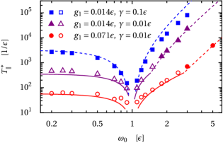
Figure 2: (Color online) Dephasing time for purely linear qubit-oscillator coupling ($g_{2}=0$), resonant driving, $\Omega=\omega_{0}$, and oscillator damping $\gamma=0.02\epsilon$. The amplitude $A=0.07\epsilon$ corresponds to the mean photon number $\bar{n}=6.125$. Filled symbols and dashed lines refer to predominantly Markovian decay, while for Gaussian decay, stroked symbols and solid lines are used.

In Fig. 2, we compare the decay time $T_{\parallel}^{*}$ with the analytical result (26) for various values of the oscillator damping and the qubit-oscillator coupling $g_{1}$ as function of the oscillator frequency. Whether Markovian or Gaussian decay dominates is visualized by filled and stroked symbols, respectively. We have skipped the regime very close to resonance, $|\lambda_{\parallel}|\lesssim 5|\omega_{0}-\epsilon|$, since there the dispersive Hamiltonian (5) is not valid and so far no dispersive readout protocol has been proposed.

Our prediction for regimes with non-Markovian decay is confirmed by the numerical solution rather well. Notice however, that in the crossover regime, our formal criterion for Markovian decay provides a unique answer, even though the respective other decay may already contribute significantly. The agreement of the numerically found border with our prediction corroborates as well the crossover time $t_{c}$ conjectured above. Concerning the values of $T_{\parallel}^{*}$, we observe a good overall agreement with the tendency that the analytical result slightly underestimates $T_{\parallel}^{*}$. In the regime of Gaussian decay, a Markov approximation would yield a significantly smaller coherence time. This means that, interestingly enough, the qubit stays coherent for a longer time than is expected from Bloch-Redfield theory. For large oscillator frequency, $\omega_{0}\gg\epsilon$, also the predicted behavior $T_{\parallel}^{*}\propto\lambda_{\parallel}^{-2}\propto|\epsilon^{2}-\omega_{0}^{2}|^{2}$ is confirmed. This substantiates the relevance of the counter-rotating correction to the dispersive shift Zueco2009b .

IV.2 Quadratic qubit-oscillator coupling $g_{2}$

We proceed as above, but consider the coupling to the square of the oscillator coordinate in the Hamiltonian (1), while setting $g_{1}=0$. Even though the linear coupling $g_{1}$ can be controlled to some extent Bertet2005a ; Bertet2005b , it is probably hard to turn it off completely. Still our choice has relevance in the limit of large detuning in which the effective dispersive coupling $\lambda_{\parallel}$ becomes rather small, see Eq. (6). Then for realistic values of $g_{2}$ for flux qubits, a protocol for recording coherent time evolution has been proposed Reuther2011b . A necessary condition for this is an oscillator bandwidth of the order of the qubit splitting, such that the oscillator does not filter out the information about the coherent qubit dynamics. Therefore, we will choose an oscillator with the rather large frequency $\Omega=\omega_{0}=5\epsilon$ and with damping up to $\gamma=\epsilon$.

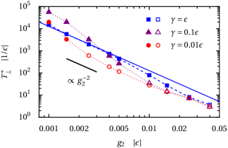
Figure 3: (Color online) Dephasing time for purely quadratic qubit-oscillator coupling ($g_{1}=0$), resonant driving at large frequency, $\Omega=\omega_{0}=5\epsilon$, and various values of the oscillator damping $\gamma$. The driving amplitude is $A=3.5\gamma$, such that always $\bar{n}=6.125$. Filled symbols mark Markovian decay, while stroked symbols refer to Gaussian shape. The solid line depicts the value obtained for $\gamma=\epsilon$ in the Markov limit. The corresponding numerical values are connected by a dashed line which serves as guide to the eye.

Figure 3 shows the numerically obtained coherence times and whether the decay is predominantly Gaussian or Markovian. For the large oscillator damping $\gamma=\epsilon$, the conditions for the validity of the (Markovian) Bloch-Redfield equation stated at the end of Sec. III.4 hold. Then we observe a good agreement of the numerically obtained $T_{\perp}^{*}$ and Eq. (29). There seems a slight systematic deviation for large values of $g_{2}$. In this limit, however, the numerical results are not very precise, because the purity falls off already during the first few oscillation periods. This rapid decay hinders a precise numerical determination of the dephasing rate. Thus, the agreement is still within the numerical precision.

For small oscillator damping, $\gamma\ll\epsilon$, Bloch-Redfield theory is not applicable, as discussed above. Moreover, the short time evolution of the purity is already too complex for a comprehensive prediction of the decoherence time. Nevertheless our numerical solution provides some hint on the decoherence process. We find that the crossover from simple exponential decay to decay with a Gaussian shape occurs at smaller values of the qubit-oscillator coupling. For small $g_{2}$, the qubit stays coherent slightly longer, while for large $g_{2}$, coherence decays a bit faster as compared to the case $\gamma=\epsilon$. In both regimes, the $\gamma$ dependence of $T_{\perp}^{*}$ is weak. This disproofs the Markovian theory for $\gamma\ll\epsilon$, because the latter predicts $T_{M}\propto 1/\gamma$, which stays in contrast to our numerical result.

V Discussion and conclusions

A qubit undergoing dispersive readout, i.e., one that is coupled to a resonantly driven dissipative harmonic oscillator, experiences decoherence from a rather exotic effective environment. The latter’s main properties stem from the small oscillator linewidth, the strong driving, and a coupling coordinate that does not commute with the qubit Hamiltonian. Nevertheless, it has been possible to analytically obtain essential and concise information about the decoherence process. Our approach is based on a transformation to the dispersive frame, which turns the linear coupling into phase noise. In doing so it is crucial to perform the transformation beyond rotating-wave approximation, in particular for studying the far detuned case where the non-rotating corrections are of the same order as the rotating-wave terms. For the subsequent analytical treatment, we have derived the dephasing time within our picture of an effective spectral density provided by the driven harmonic oscillator in the semiclassical limit. At the same time it has turned out that a peaked spectral density induces a generally non-Markovian dissipative dynamics.

As a main finding of this work, we have pointed out that the decoherence process happens in two stages. In the beginning, the purity decays like a Gaussian, while subsequently, Markovian decay sets in. If the qubit-oscillator coupling is strong or if the oscillator is strongly driven, the major part of the coherence decays already during the first stage such that the relevant dynamics possesses a Gaussian time profile. Thus, with the trend towards ultra-strong coupling between a qubit and a harmonic mode Devoret2007a ; Anappara2009a ; Niemczyk2010a ; Ashhab2010a , Gaussian decay should become increasingly relevant. In the opposite limit of weak coupling, the first stage reduces the qubit coherence only by a small amount, rendering the relevant decoherence Markovian. The dephasing times in the two regimes exhibit distinct parameter dependencies, which we have determined analytically. Remarkably, in the Gaussian regime, the coherence time may be significantly longer than what one would expect from an extrapolation of the Markovian result.

For a numerical description of the dynamics, we have solved the full Bloch-Redfield master equation for the qubit coupled to the driven oscillator in the frame of the original Hamiltonian. This has allowed us to obtain numerical results that are fully independent of the analytical treatment. They have confirmed our predictions for the partially non-Markovian purity decay for the case of linear qubit-oscillator coupling. For quadratic coupling, the decoherence process is more involved. Nevertheless, it has been possible to obtain an analytical expression for the decoherence rate in the Markovian limit. Beyond this limit, our numerical solution indicates that decoherence is non-Markovian provided that the oscillator dissipation is very weak.

Finally, we are convinced that our results on the decoherence induced by a resonantly driven oscillator will support the design of future experiments with dispersive readout and its generalizations.

Appendix A The driven dissipative harmonic oscillator

A.1 Markovian master equation

In the absence of the qubit and for sufficiently weak oscillator-bath coupling, the dissipative dynamics of the oscillator is well described within Bloch-Redfield theory Redfield1957a ; Blum1996a . Since additive driving of the form (3) does not influence the dissipative terms Kohler1997a , it is possible to use the master equation for the undriven dissipative harmonic oscillator and to simply add the time-dependent Hamiltonian (3), such that

$$\begin{split}\dot{\rho}_{\text{osc}}=&-i\omega_{0}[a^{\dagger}a,\rho_{\text{osc}}]-\frac{i}{\hbar}[H_{F}(t),\rho_{\text{osc}}]\\ &-\frac{i\gamma}{2}[x,[p,\rho_{\text{osc}}]_{+}]-\frac{\gamma}{2}\coth\Big{(}\frac{\hbar\omega_{0}}{2k_{B}T}\Big{)}[x,[x,\rho_{\text{osc}}]].\end{split}$$ (30)

A.2 Average position

Owing to the linearity of the quantum Langevin equation for the dissipative harmonic oscillator, its position expectation value $\bar{x}$ obeys the classical equation of motion

$$\ddot{\bar{x}}+\gamma\dot{\bar{x}}+\omega_{0}^{2}\bar{x}=\omega_{0}F(t).$$ (31)

The response $\bar{x}(t)$ to the driving is most conveniently obtained by a time convolution with the Green’s function $G(t)$, where

$$G(\omega)=\frac{\omega_{0}}{-\omega^{2}-i\gamma\omega+\omega_{0}^{2}},$$ (32)

and the inhomogeneity $F(t)$. For $F(t)=A\cos(\Omega t-\phi_{0})$, the solution reads

$$\bar{x}(t)=|G(\Omega)|A\cos(\Omega t-\phi-\phi_{0}),$$ (33)

where the phase shift $\phi$ is the argument of the Green’s function. The corresponding semiclassical state is a coherent state with mean photon number $\bar{n}=\frac{1}{2}A^{2}|G(\Omega)|^{2}$.

A.3 Position correlation function

In the Markovian limit for the undriven dissipative harmonic oscillator implied in the master equation (30) in the absence of $H_{F}$, the equilibrium position auto-correlation function

$$S_{\delta x\,\delta x}(t)=\frac{1}{2}\langle\delta[x(t),\delta x(0)]_{+}\rangle$$ (34)

can be computed by help of the quantum regression theorem Lax1963a . It essentially states that $S_{\delta x\,\delta x}$ obeys the same equation of motion as the average position. Thus,

$$\ddot{S}_{\delta x\,\delta x}+\gamma\dot{S}_{\delta x\,\delta x}+\omega_{0}^{2}S_{\delta x\,\delta x}=0.$$ (35)

The initial value is

$$S_{\delta x\,\delta x}\big{|}_{t=0}=\frac{1}{2}\coth\Big{(}\frac{\hbar\omega_{0}}{2k_{B}T}\Big{)},$$ (36)

while for symmetric ordering, its time derivative at $t=0$ vanishes. Thus, we can express the solution as Fourier integral of the Green’s function (32) which we evaluate via Cauchy’s theorem. In the weak damping limit considered herein, $\gamma\ll\omega_{0}$, we neglect the dissipation induced frequency shift and continue with the approximation

$$S_{\delta x\,\delta x}(t)=\frac{1}{2}\coth\Big{(}\frac{\hbar\omega_{0}}{2k_{B}T}\Big{)}e^{-\gamma t/2}\cos(\omega_{0}t).$$ (37)

References

- (1) M. A. Nielsen and I. L. Chuang, Quantum Computing and Quantum Information (Cambridge University Press, Cambridge, 2000)
- (2) I. Chiorescu, P. Bertet, K. Semba, Y. Nakamura, C. J. P. M. Harmans, and J. E. Mooij, Nature (London) 431, 159 (2004)
- (3) A. Wallraff, D. I. Schuster, A. Blais, L. Frunzio, R.-S. Huang, J. Majer, S. Kumar, S. M. Girvin, and R. J. Schoelkopf, Nature (London) 431, 162 (2004)
- (4) M. Grajcar, A. Izmalkov, E. Il’ichev, T. Wagner, N. Oukhanski, U. Hübner, T. May, I. Zhilyaev, H. E. Hoenig, Ya. S. Greenberg, V. I. Shnyrkov, D. Born, W. Krech, H.-G. Meyer, A. Maassen van den Brink, and M. H. S. Amin, Phys. Rev. B 69, 060501(R) (2004)
- (5) M. A. Sillanpää, T. Lehtinen, A. Paila, Y. Makhlin, L. Roschier, and P. J. Hakonen, Phys. Rev. Lett. 95, 206806 (2005)
- (6) A. Lupascu, E. F. C. Driessen, L. Roschier, C. J. P. M. Harmans, and J. E. Mooij, Phys. Rev. Lett. 96, 127003 (2006)
- (7) D. I. Schuster, A. A. Houck, J. A. Schreier, A. Wallraff, J. M. Gambetta, A. Blais, L. Frunzio, J. Majer, B. Johnson, M. H. Devoret, S. M. Girvin, and R. J. Schoelkopf, Nature (London) 445, 515 (2007)
- (8) A. Blais, R.-S. Huang, A. Wallraff, S. M. Girvin, and R. J. Schoelkopf, Phys. Rev. A 69, 062320 (2004)
- (9) D. Zueco, G. M. Reuther, S. Kohler, and P. Hänggi, Phys. Rev. A 80, 033846 (2009)
- (10) G. M. Reuther, D. Zueco, P. Hänggi, and S. Kohler, New J. Phys. 13, 093022 (2011)
- (11) G. M. Reuther, D. Zueco, P. Hänggi, and S. Kohler, Phys. Rev. Lett. 102, 033602 (2009)
- (12) G. M. Reuther, D. Zueco, P. Hänggi, and S. Kohler, Phys. Rev. B 83, 014303 (2011)
- (13) A. A. Clerk, M. H. Devoret, S. M. Girvin, F. Marquardt, and R. J. Schoelkopf, Rev. Mod. Phys. 82, 1155 (2010)
- (14) A. G. Redfield, IBM J. Res. Develop. 1, 19 (1957)
- (15) K. Blum, Density Matrix Theory and Applications, 2nd ed. (Springer, New York, 1996)
- (16) M. Thorwart, E. Paladino, and M. Grifoni, Chem. Phys. 296, 333 (2004)
- (17) F. Nesi, M. Grifoni, and E. Paladino, New. J. Phys. 9, 316 (2007)
- (18) A. Garg, J. N. Onuchic, and V. Ambegaokar, J. Chem. Phys. 83, 4491 (1985)
- (19) L. Tian, S. Lloyd, and T. P. Orlando, Phys. Rev. B 65, 144516 (2002)
- (20) C. H. van der Wal, F. K. Wilhelm, C. J. P. M. Harmans, and J. E. Mooij, Eur. Phys. J. B 31, 111 (2003)
- (21) M. Devoret, S. Girvin, and R. Schoelkopf, Ann. Phys. 16, 767 (2007)
- (22) A. A. Anappara, S. De Liberato, A. Tredicucci, C. Ciuti, G. Biasiol, L. Sorba, and F. Beltram, Phys. Rev. B 79, 201303(R) (2009)
- (23) S. Ashhab and F. Nori, Phys. Rev. A 81, 042311 (2010)
- (24) T. Niemczyk, F. Deppe, H. Huebl, E. P. Menzel, F. Hocke, M. J. Schwarz, J. J. García-Ripoll, D. Zueco, T. Hümmer, E. Solano, A. Marx, and R. Gross, Nature Phys. 6, 772 (2010)
- (25) M. Boissonneault, J. M. Gambetta, and A. Blais, Phys. Rev. A 77, 060305 (2008)
- (26) M. Boissonneault, A. C. Doherty, F. R. Ong, P. Bertet, D. Vion, D. Esteve, and A. Blais, Phys. Rev. A 85, 022305 (2012)
- (27) P. Bertet, I. Chiorescu, G. Burkard, K. Semba, C. J. P. M. Harmans, D. P. DiVincenzo, and J. E. Mooij, Phys. Rev. Lett. 95, 257002 (2005)
- (28) P. Bertet, I. Chiorescu, C. J. P. M. Harmans, and J. E. Mooij, “Dephasing of a flux-qubit coupled to a harmonic oscillator,” arXiv:cond-mat/0507290 (2005)
- (29) S. Kohler, T. Dittrich, and P. Hänggi, Phys. Rev. E 55, 300 (1997)
- (30) M. Boissonneault, J. M. Gambetta, and A. Blais, Phys. Rev. A 79, 013819 (2009)
- (31) G. M. Reuther, D. Zueco, F. Deppe, E. Hoffmann, E. P. Menzel, T. Weißl, M. Mariantoni, S. Kohler, A. Marx, E. Solano, R. Gross, and P. Hänggi, Phys. Rev. B 81, 144510 (2010)
- (32) M. Lax, Phys. Rev. 129, 2342 (1963)
- (33) H.-P. Breuer and F. Petruccione, Theory of open quantum systems (Oxford University Press, Oxford, 2003)
- (34) Y. Makhlin and A. Shnirman, Phys. Rev. Lett. 92, 178301 (2004)
- (35) G. Falci, A. D’Arrigo, A. Mastellone, and E. Paladino, Phys. Rev. A 70, 040101(R) (2004)
- (36) G. Falci, A. D’Arrigo, A. Mastellone, and E. Paladino, Phys. Rev. Lett. 94, 167002 (2005)
- (37) Y. Matsuzaki, S. Saito, K. Kakuyanagi, and K. Semba, Phys. Rev. B 82, 180518(R) (2010)
- (38) K. M. Fonseca-Romero, S. Kohler, and P. Hänggi, Chem. Phys. 296, 307 (2004)