Dynamics of bimodality in vehicular traffic flows

Abstract

A model equation has been proposed to describe bimodal features in vehicular traffic flows. The dynamics of the bimodal distribution reveals the existence of a fixed point that is connected to itself by a homoclinic trajectory. The mathematical conditions associated with bimodality have been established. The critical factors necessary for both a breaking of symmetry and a transition from bimodal to unimodal behaviour, in the manner of a bifurcation, have been analysed.

I Introduction

Bimodal distributions are characterised by the existence of two distinct modes (peaks) in a single frequency distribution Ross (2004). Usually such a distribution is seen as a mixture of two normal distributions. Standard methods to understand bimodal distributions take recourse to statistical methods, and it is only rarely that a model of bimodality is provided Dallavalle et al. (1951). In keeping with the latter principle, the primary emphasis of this work is on developing a mathematical model that will give a single global description of bimodal phenomena. The model proposed here has been structured on the bimodal distribution of data pertaining to vehicular traffic flows, which is a man-made condition, although bimodal features are exhibited in many natural phenomena as well Guthrie (1982); Choi and Herbst (1996); Cochran et al. (2004). From a purely mathematical perspective, however, the scope of the model goes much beyond any particular practical context.

The model has been used to understand the dynamics underlying a bimodal distribution, following standard methods of nonlinear dynamics Strogatz (1994); Jordan and Smith (1999). In so doing, the dependence of bimodal properties on various parameters has been brought to the fore. The dynamics of the model bimodal distribution reveals that the controlling parameters can be adjusted to cause bimodal-to-unimodal transition (like a bifurcation) and a breaking of symmetry in the system (both of which have been seen in some previous studies on bimodality Chechkin et al. (2003); Dybiec and Gudowska-Nowak (2007)).

II Bimodality in Vehicular Traffic Flows

Nowadays the number of vehicles on the roads has increased prodigiously, along with an accompanying necessity to expand road networks. Any implementation of an advanced transportation system, therefore, needs a clear view of the present intricacies in traffic flows. Studies of vehicular traffic flows usually aim at understanding interactions among streams of vehicles (modelled occasionally as particles), and a substantial body of relevant work, ranging across multiple perspectives, has already come into existence Chowdhury et al. (2000); Helbing (2001); Waldeer (2003, 2004); del Rio and Larraga (2005); Kaupuzs et al. (2005); Maerivoet and Moor ; Helbing et al. (2005); Maerivoet and Moor (2005); Chakrabarti (2006); Reichenbach et al. (2007); Appert-Rolland (2009); Gershenson ; Champagne et al. ; Pradhan et al. (2010); Appert-Rolland et al. (2010); Gershenson and Rosenblueth (2011); de Gier et al. (2011); Neri et al. (2011); Ding and Ding (2012). The practical motive behind these studies is to eliminate the problem of traffic congestion, and to devise effective methods of controlling traffic flow.

The mathematical model in this work takes a macroscopic view of the vehicular traffic of a city at a given hour in the day — in effect, the bulk of traffic as a function of time. The data needed for the purpose of modelling have been taken from the repository of the Alabama Department of Transportation (ALDOT) , and the particular city whose traffic data have been used here, is Jackson in Alabama State, USA. The principal factor guiding the choice of this city is that with Jackson being comparatively small in size, the data about its traffic have been systematically recorded, and are free of the usual complications associated with the traffic of very large cities. This has the advantage of simplicity, where placing the foundations of a mathematical model is concerned.

The Jackson data indicate that the bulk traffic is dominated by flows in the eastward and westward directions. The plot of the data for the westward traffic is shown in Fig. 1, with the broken line. Similarly, the plot of the eastward traffic is shown in Fig. 2. In both these plots, the time, $t$, at which the traffic volume, $N\left(t\right)$, was measured, has been scaled so that $t=0$ coincides with midday, $12$:$00$ hours. This enables one to take advantage of any possible symmetry in the distribution of the data, especially if there is a symmetry about $t=0$. From a look at both Figs. 1 & 2, however, only an asymmetric bimodal distribution is to be seen, with two peaks of unequal height in either plot. What Fig. 1 suggests is that the morning traffic volume is much higher in the western direction than in the opposite direction, while the behaviour of the bimodal curve in Fig. 2 is quite the opposite, with the eastward traffic being disproportionately high in the evening. There is a clear commuter preference in the traffic flow as a function of time.

Extraneous traffic (due to vehicles coming from outside the city, passing through it, and leaving it ultimately) may add to the count of the indigenous traffic flow. One may imagine Jackson city as a bounded volume, through which there occurs a bulk flow of traffic from the rest of the world. This flow is bi-directional, and along either direction the external traffic volume maintains a uniform average value. Besides, whatever goes into this bounded system at one end, also comes out of the other end in finite time. Consequently, the alien traffic does not cause any appreciable bias in the bimodal distribution. The variation in the data around this constant background of global traffic, is then due only to the local city traffic, which oscillates back and forth between the eastern and western boundaries, once in a cycle of twenty four hours.

Social and economic conditions also have a major role to play in the way the data are distributed from one day of the week to the other. The weekend traffic (on Saturdays and Sundays) will follow a different pattern, in comparison to the traffic on a working day. And even on working days close to the weekend, like Mondays and Fridays, the traffic flow may be different from what it would be in the middle of the week. So a judicious choice of the data has to be made here. For the purpose of crafting a mathematical model from first principles, the data employed in this work are the average values of all the Wednesday traffic data of Jackson city in the year, $2007$. Wednesday is in the middle of the week, and it is in this period of the week that all city traffic is expected to rid itself of the weekend effect and reach a local mid-week equilibrium. So the corresponding data should convey more unambiguous trends in the traffic flow.

III A Mathematical Model for Bimodality

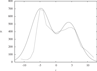
Figure 1: Bimodal distribution of traffic flow due west. The vertical axis measures the volume of traffic, $N$, for a given time, $t$ (scaled in hours). The horizontal axis has been scaled so that $t=0$ is set at midday, $12$:$00$ hours. The dotted broken curve joins the real data points, and the continuous curve traces the model given by Eq. (2). The parameter values used for the fit are $A=44.0$, $\mu=8.53$, $\lambda=0.19$ and $\beta=-0.09$.

Figure 2: Bimodal distribution of traffic flow due east. The plotting follows the same principles outlined in Fig. 1, but the parameter values necessary for fitting the data are $A=44.1$, $\mu=10.5$, $\lambda=0.22$ and $\beta=0.24$. The sign and the absolute magnitude of $\beta$ make the most significant difference between the two bimodal distributions.

The continuous curves in Figs. 1 & 2 follow the model function that describes bimodal distributions. In such distributions one encounters three turning points. So it is natural to suggest that a fourth-degree (quartic) polynomial Chechkin et al. (2003); Dybiec and Gudowska-Nowak (2007), whose derivative is of the third degree (cubic), will correspond to the three turning points. This particular feature can be captured by an “inverted Mexican hat”-type function of the form, $N\left(t\right)=a+t^{2}-bt^{4}$, in which $N$ is volume of the traffic flow and $t$ is the hour at which the traffic flow has been measured. The discrepancy between this function and the pattern followed by the data, however, lies in the asymptotic conditions of the latter. Both the inner and the outer time limits on the horizontal axis in Figs. 1 & 2, are close to midnight. At that hour, on a working day in the middle of the week, the volume of traffic trickles down to small values, a condition that should be described mathematically by a function with an asymptotic decay, $N\longrightarrow 0$, at the extreme ends of the time axis. And this is how it should be, because a bimodal distribution is usually treated as a mixture of two normal distributions, which have a similarly decaying tail. This, however, is not indicated by the “inverted Mexican hat” function, which intersects the line $N=0$ in finite time.

To capture the required asymptotic behaviour of the bimodal distribution, therefore, it is expedient to employ a Maxwell-Boltzmann type of function in the form, $N\left(t\right)=\alpha\left(\mu+t^{2}\right)\exp\left(-\lambda^{2}t^{2}\right)$. From the foregoing function, for low values of $t$, on approximating $\exp\left(-\lambda^{2}t^{2}\right)\simeq 1-\lambda^{2}t^{2}$, one recovers the features of the “inverted Mexican hat” function. Another aspect of the Maxwell-Boltzmann distribution is that its integral (the area under the curve) is constant, in consonance with the fact that in an average sense the total volume of the internal city traffic is constant over one full day.

With the required asymptotic condition satisfied thus, the role of the parameter, $\mu$, can now be examined. From the Maxwell-Boltzmann function, setting its time derivative, $\dot{N}=0$, one obtains the condition, $t\left[1-\lambda^{2}\left(\mu+t^{2}\right)\right]=0$, which indicates three turning points in time, at $t=0$ and $t=\pm\left(\lambda^{-2}-\mu\right)^{1/2}$. Now, the two non-zero roots of $t$ can only be real when $\mu<\lambda^{-2}$. When $\mu=\lambda^{-2}$, all the three roots coalesce at $t=0$. Noting that bimodality implies the existence of three turning points, the importance of the parameter $\mu$ in maintaining bimodality is now evident.

The distribution traced out by the Maxwell-Boltzmann function is, however, symmetric about $t=0$, which is certainly not to be expected in a real bimodal distribution. And more to the point for traffic flows, this lack of symmetry is exchanged over a time scale of half a day, as it has been shown in Figs. 1 & 2. While the traffic due west is higher in the morning hour than at any other time of the day, the traffic due east displays an exact reversal of this trend. To account for these two features, two new parameters, $\gamma$ and $\sigma$, are now introduced to break the symmetry of the Maxwell-Boltzmann distribution, which, consequently, goes as

$$N\left(t\right)=\alpha\left(\mu+t^{2}\right)\exp\left(-\lambda^{2}t^{2}\right)\left(1+\gamma\right)^{\sigma t}\,.$$ (1)

Any non-zero value of $\gamma$ in the foregoing expression will raise one peak in the bimodal distribution, and lower the other, i.e. break the symmetry about $t=0$ in Figs. 1 & 2. Symmetry is, of course, restored when $\gamma=0$, and in this special case, Eq. (1) assumes the general mathematical form of the energy eigenfunction of the second state of the linear harmonic oscillator Schiff (1968). When $\gamma\neq 0$, the part played by $\sigma$ in the distribution given by Eq. (1) is to exchange the respective positions of the two uneven peaks, depending on the direction of the traffic flow, a condition that can be achieved simply by assigning the values, $\sigma=\pm 1$.

With all the parameter values specified suitably, Eq. (1) can be used to fit the data, but a transformation of it helps in reducing the number of parameters in the model. Accordingly, Eq. (1) is recast as

$$N(t)=A\left(\mu+t^{2}\right)\exp\left[-\left(\lambda t-\beta\right)^{2}\right]\,,$$ (2)

in which $\beta=\sigma\left(2\lambda\right)^{-1}\ln\left(1+\gamma\right)$ and $A=\alpha\exp\left(\beta^{2}\right)$. Now $\beta$, having taken over the roles of $\gamma$ and $\sigma$, controls both the breaking of symmetry and the exchange of the peaks in the bimodal curve. The former condition is obtained from the absolute magnitude of $\beta$, while the latter from its sign. These values, as well as values of $A$, $\mu$ and $\lambda$ are used to fit the data, as shown in Figs. 1 & 2.

IV Dynamics of Bimodality

The model for the data fit, as given by Eq. (2), is in the form, $N\equiv N\left(t\right)$. Two parameters in this model, $\mu$ and $\beta$, play a crucial part in causing an asymmetric bimodality. For certain values of these parameters (for instance $\mu=\lambda^{-2}$ and $\beta=0$), the bimodal distribution undergoes qualitative changes. To investigate these aspects of the model in detail, it will be necessary to find $\dot{N}$, and then to plot a phase portrait, $N$–$\dot{N}$. This will reveal much about the stability, creation and annihilation of the turning points, and also the properties of any possible fixed point(s) in the bimodal system Strogatz (1994); Jordan and Smith (1999). So going back to Eq. (2), its first derivative in time (indicated by an overdot) is obtained in a non-autonomous form as

$$\dot{N}=2\left[\frac{t}{\mu+t^{2}}-\lambda\left(\lambda t-\beta\right)\right]N\,.$$ (3)

Turning points are given by the condition $\dot{N}=0$. In addition to this requirement, fixed points are obtained when $\ddot{N}=0$ Jordan and Smith (1999). So to know the conditions needed for determing the fixed points of the system, the second time derivative of the function, $N\equiv N\left(t\right)$, is obtained and set down in a non-autonomous form as

$$\ddot{N}=2\left[\frac{1-4\lambda t\left(\lambda t-\beta\right)}{\mu+t^{2}}+2\lambda^{2}\left(\lambda t-\beta\right)^{2}-\lambda^{2}\right]N\,.$$ (4)

Both Eqs. (3) and (4) indicate the existence of a fixed point at $N=N^{\star}=0$, when the conditions $\ddot{N}=\dot{N}=0$ are simultaneously satisfied. This fixed point is obtained, going by Eq. (2), when $t\longrightarrow\pm\infty$. The existence of other fixed points will depend on whether or not Eqs. (3) and (4) will have common roots in $t$ when $\ddot{N}=\dot{N}=0$. Solving for $t$ under these conditions will show how $\mu$ and $\beta$ influence the dynamics of the bimodal system.

The role that $\mu$ plays can be known clearly by considering the limiting case of $\beta=0$. In this perfectly symmetric limit, on solving the explicitly time-dependent part of $\dot{N}=0$, three roots of $t$ are obtained, one at $t=0$ and the other two at $t=\pm\left(\lambda^{-2}-\mu\right)^{1/2}$. None of these three roots of $t$ leads to $\ddot{N}=0$. The only conclusion that can be drawn from this fact is that there is only one fixed point in the bimodal system, at $N=N^{\star}=0$. All other solutions of $\dot{N}=0$ give only turning points in the bimodal system. For $t=0$ one obtains a turning point of $N$ at $N_{0}=A\mu$, as it can be seen from Eq. (2). The two non-zero roots of $t$ at $t=\pm\left(\lambda^{-2}-\mu\right)^{1/2}$, will give two coinciding turning points on the line $\dot{N}=0$, in the phase portrait. From Eq. (2), these two turning points are to be found at $N_{\mathrm{T}}=A\lambda^{-2}\exp\left(\mu\lambda^{2}-1\right)$. To have three real roots of $t$, it is necessary to fulfil the condition, $\mu<\lambda^{-2}$. By means of this condition it can also be argued that $N_{\mathrm{T}}>N_{0}$. Hence, as long as $\mu<\lambda^{-2}$, there shall remain three turning points, one at $N=N_{0}$ and the other two coinciding at $N=N_{\mathrm{T}}$. As $\mu\longrightarrow\lambda^{-2}$, these two turning point positions approach each other in the $N$–$\dot{N}$ phase portrait. When $\mu=\lambda^{-2}$, there is a bifurcation-like behaviour because of which the turning point at $N_{0}$ and one of the turning points at $N_{\mathrm{T}}$ annihilate each other. What survives this mutual annihilation is the second “concealed” turning point at $N_{\mathrm{T}}$. Subsequently, for $\mu>\lambda^{-2}$, only this turning point will continue its existence, and the distribution will become unimodal.

The entire sequence of this behaviour of the turning points over the range, $0<\mu<\lambda^{-2}$, has been depicted in Fig. 3. It is evident from this plot that bimodality is closely related to the existence of a closed loop for a phase trajectory in the $N$–$\dot{N}$ portrait. This is one clear message that has emerged from the phase-portrait analysis. When $\mu\longrightarrow 0$, bimodality becomes very pronounced, and when $\mu\longrightarrow\lambda^{-2}$, bimodality becomes progressively enfeebled, disappearing altogether when $\mu=\lambda^{-2}$. In the former case, the sole fixed point at $N=N^{\star}=0$ coincides with the turning point, $N_{0}=0$, while in the latter case, bimodality is eradicated because of a mutual annihilation between the turning points, $N_{0}\left(\neq 0\right)$ and $N_{\mathrm{T}}$. Once bimodality disappears and the distribution becomes unimodal, another fact that stands out clearly through the phase-portrait analysis is the existence of a homoclinic trajectory that joins the fixed point, $N^{\star}=0$, to itself. Also, the closed loop that traces bimodality in the phase portrait indicates a local periodic behaviour (which effectively implies that the two peaks in the bimodal distribution give a local scale), and when $\mu\longrightarrow 0$, this local periodicity of what is now a strongly bimodal system, takes place on a time scale of $\lambda^{-1}$.

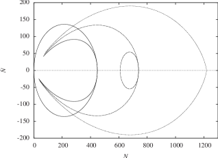
Figure 3: A symmetric phase portrait (with $\beta=0$), using the parameter values of $A$ and $\lambda$ taken from Fig. 1. When $\mu=0$, the phase trajectories are shown by the continuous curve at the extreme left. The closed loop has the largest area in this case. When $\mu=0.5\lambda^{-2}$, the loop size shrinks, as the dotted curve shows in the centre of the plot. When $\mu=\lambda^{-2}$, the loop vanishes as the curve on the extreme right shows. The existence of a closed loop in the plots above is a signature of bimodality. When $\mu=\lambda^{-2}$, a bimodal-to-unimodal transition occurs, and the closed loop disappears, i.e. bimodality is lost. All along there is a fixed point at $N=\dot{N}=0$, joined to itself by a homoclinic trajectory.

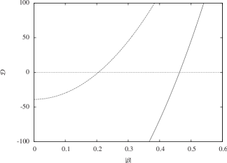
Figure 4: When symmetry is broken (for $\beta\neq 0$), there are three distinct turning points for $\dot{N}=0$. When the asymmetry is large, two of these fixed points are lost due to a bimodal-to-unimodal transition. This happens when the discriminant of Eq. (6), $\mathcal{D}=0$. The variation of $\mathcal{D}$ against $|\beta|$ (since $\beta<0$ for the westward traffic) shows that the transition occurs when $|\beta|=|\beta_{\mathrm{b}}|\simeq 0.21$ for the eastward traffic (traced by the dotted curve), and when $|\beta|=|\beta_{\mathrm{b}}|\simeq 0.46$ for the westward traffic (the continuous curve). For both of these cases the values of $\mu$ and $\lambda$ are what they are for Figs. 1 & 2, respectively.

The next effect to consider is the one of breaking the symmetry corresponding to $\beta=0$. The first thing to happen when $\beta\neq 0$, is that the two hitherto coinciding turning points at $N=N_{\mathrm{T}}$ are separated from each other. A simple perturbative argument suffices to establish this. If $\beta\ll 1$, then about the turning point $N_{\mathrm{T}}$ (determined for $t^{2}=\lambda^{-2}-\mu$), it is possible to linearise all terms involving $\beta$ in Eq. (2), and obtain the two separated roots as $N_{{\mathrm{T}}\pm}\simeq N_{\mathrm{T}}\left[1\pm 2\beta\left(1-\mu\lambda^{2}\right)^{1/2}\right]$.

As $\beta$ increases in magnitude, the position of $N_{{\mathrm{T}}+}$ shifts to higher values of $N$ on the line $\dot{N}=0$, while the position of $N_{{\mathrm{T}}-}$ slides in the opposite direction. This pair of roots corresponds to the two asymmetric peaks in the bimodal curve, with $N_{{\mathrm{T}}+}$ tracing the locus of the higher peak, and $N_{{\mathrm{T}}-}$ the lower. Between the two of them, these peaks flank a point of local minimum in the bimodal distribution, which itself turns out to be the third turning point on the line, $\dot{N}=0$. When $\beta=0$, this point is at $N=N_{0}$, with $N_{0}<N_{\mathrm{T}}$, but when $\beta\neq 0$, the position of this third unpaired turning point shifts to larger values of $N$, and for sufficiently high values of $\beta$, it suffers a separate pair annihilation with the shifting turning point at $N_{{\mathrm{T}}-}$. This reasoning is borne out by solving for $\dot{N}=0$ in Eq. (3), specifically its non-autonomous, time-dependent part. What transpires is a third-order polynomial in the variable $t$, which goes as

$$t^{3}-\left(\frac{\beta}{\lambda}\right)t^{2}-\left(\frac{1}{\lambda^{2}}-\mu\right)t-\frac{\mu\beta}{\lambda}=0\,.$$ (5)

Performing a variable transformation, $t=\tau+h$, in the preceding relation, and setting $h=\beta\left(3\lambda\right)^{-1}$, one obtains the canonical form of a cubic equation,

$$\tau^{3}+{\mathcal{P}}\tau+{\mathcal{Q}}=0\,,$$ (6)

whose analytical roots are extracted by the application of the Cardano-Tartaglia-del Ferro method. Noting that

$${\mathcal{P}}=\mu-\frac{1}{\lambda^{2}}\left(1+\frac{\beta^{2}}{3}\right),\,{\mathcal{Q}}=-\frac{\beta}{3\lambda}\left(\frac{2\beta^{2}+9}{9\lambda^{2}}+2\mu\right),$$

the discriminant of the cubic equation is

$${\mathcal{D}}=\frac{\mathcal{Q}^{2}}{4}+\frac{\mathcal{P}^{3}}{27}\,.$$ (7)

The sign of $\mathcal{D}$ is crucial here. If $\mathcal{D}>0$, there will be only one real root of $\tau$ (the other two being complex, which are known to occur in pairs). On the other hand, if $\mathcal{D}<0$, all the three roots of $\tau$ will be real. Knowing $\tau$, leads easily to knowing $t$, which, on using Eq. (2), gives the corresponding value of $N$. This is a turning point on the line $\dot{N}=0$. If there are three real roots of $\tau$ (for $\mathcal{D}<0$), then there will be three turning points of $N\left(t\right)$. If, however, there is only one real root of $\tau$ (for $\mathcal{D}>0$), then there will be only one turning point of $N\left(t\right)$, the other two having been annihilated on the line, $\dot{N}=0$.

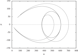
Figure 5: Phase plot of the bimodal distribution of the traffic flow due west. Both the curves are plotted for the values of $A$, $\mu$ and $\lambda$ used in Fig. 1. When $\beta=0$, the resulting plot is shown by the continuous symmetric curve. When $\beta=-0.09$ (as in Fig. 1), asymmetry sets in, as shown by the dotted curve.

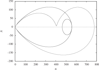
Figure 6: Phase plot of the bimodal distribution of the traffic flow due east. The plotting here follows the scheme of Fig. 5. Both the curves are plotted for the values of $A$, $\mu$ and $\lambda$ used in Fig. 2. The continuous curve shows the symmetric case (for $\beta=0$), while the asymmetric dotted curve is plotted for $\beta=0.24$ (as in Fig. 2). Since this value of $\beta>|\beta_{\mathrm{b}}|$ (the latter value is to be read from Fig. 4), a bimodal-to-unimodal transition has already taken place, and instead of a closed loop on the dotted curve, all that remains is a cusp just above the line, $\dot{N}=0$.

Evidently, a critical condition is reached when $\mathcal{D}=0$, i.e. when a bimodal-to-unimodal transition occurs. This might be viewed as a bifurcation in the bimodal system, for the value of $\beta=\beta_{\mathrm{b}}$. To understand how asymmetry in the bimodal distribution brings about this type of bifurcation behaviour, one needs to follow how $\mathcal{D}$ depends on $\beta$. This variation has been plotted in Fig. 4, using the values of $\mu$ and $\lambda$ needed to calibrate the data of both the east and west-moving traffic. Considering $|\beta|$ (since $\beta<0$ for the west-going traffic), a transition from a bimodal distribution to a unimodal distribution (or vice versa) can be seen to take place (when $\mathcal{D}=0$) for $|\beta_{\mathrm{b}}|\simeq 0.21$ in the case of the eastward traffic, and for $|\beta_{\mathrm{b}}|\simeq 0.46$ in the case of the westward traffic.

Going back to Figs. 1 & 2, one can see from the former plot, the value of $|\beta|$ needed to fit the data ($|\beta|=0.09$) is much less than what can cause the bimodal-unimodal bifurcation ($|\beta_{\mathrm{b}}|\simeq 0.46$), while in the latter plot the reverse is true (here $|\beta_{\mathrm{b}}|\simeq 0.21<|\beta|=0.24$). The consequence of this is that, as opposed to Fig. 1, no conspicuous secondary peak in the bimodal distribution is seen in Fig. 2. The implications of both these conditions, as far as the dynamics on the $N$–$\dot{N}$ phase portrait is concerned, have been shown in Figs. 5 & 6. These two plots show the dynamics of bimodality for the west-moving and the east-moving traffic, respectively. In both the cases, when $\beta=0$, there is a point on the line $\dot{N}=0$, where the curve loops over itself. The shifting of this point away from the aforesaid line, suggests breaking of symmetry and asymmetric bimodality. For $\beta<0$ (westward traffic), this point shifts below the line, while for $\beta>0$ (eastward traffic), the point shifts above. So to give a succinct description, it can be said that $\mu$ causes bimodality, and $\beta$ causes a breaking of symmetry. Taking these two aspects of the two parameters together, what results is an asymmetric bimodality. And changing the values of both these parameters can cause a bimodal-to-unimodal transition in the distribution, much in the likeness of a bifurcation.

V Concluding Remarks

The dynamics and the phase-portrait analysis, based on the model equation for bimodal behaviour, have helped in unearthing some general properties of a bimodal distribution. The first is that the signature of bimodality in a phase-portrait is the existence of a closed loop, and the second is the existence of a homoclinic trajectory, connecting a lone fixed point to itself in the phase portrait. Arguably, these are features which will hold true in other types of bimodal distribution as well. Although the primary emphasis of this study is to understand the generic mathematical features of bimodality, its practical implications might help in designing innovative traffic control mechanisms, and afford a new perspective on addressing traffic-related problems.

The model developed here is based on a relatively uncomplicated bi-directional flow of traffic along one axis only (in this case, east to west and vice versa). There is scope for refinement, when one considers the complications associated with the vast traffic networks of very big cities. A large vehicular traffic flow in a particular direction is the outcome of global decision patterns of commuters. In addition, traffic flows depend on routing possibilities in a traffic network, as well as on congestions that can occur in that network. In other words, the physics of vehicular traffic flows is associated with a complex dynamic competition between the demand for traffic space and its availability. The bimodal pattern studied here gives a simple one-dimensional perspective of this complex structure and its dynamics. With the aid of advanced modelling techniques, it should become possible to simulate and analyse these conditions, for which data may not be available, or for situations in which it may be difficult to perform realistic experiments on large scales. All of these should go a long way in building a generalised model that could be applied to traffic flows in an arbitrarily structured network.