Modeling the X-rays Resulting From High Velocity Clouds

Abstract

With the goal of understanding why X-rays have been reported near some high velocity clouds, we perform detailed 3 dimensional hydrodynamic and magnetohydrodynamic simulations of clouds interacting with environmental gas like that in the Galaxy’s thick disk/halo or the Magellanic Stream. We examine 2 scenarios. In the first, clouds travel fast enough to shock-heat warm environmental gas. In this scenario, the X-ray productivity depends strongly on the speed of the cloud and the radiative cooling rate. In order to shock-heat environmental gas to temperatures of $\geq 10^{6}$ K, cloud speeds of $\geq 300$ km/s are required. If cooling is quenched, then the shock-heated ambient gas is X-ray emissive, producing bright X-rays in the 1/4 keV band and some X-rays in the 3/4 keV band due to O VII and other ions. If, in contrast, the radiative cooling rate is similar to that of collisional ionizational equilibrium plasma with solar abundances, then the shocked gas is only mildly bright and for only about 1 Myr. The predicted count rates for the non-radiative case are bright enough to explain the count rate observed with XMM-Newton toward a Magellanic Stream cloud and some enhancement in the ROSAT 1/4 keV count rate toward Complex C, while the predicted count rates for the fully radiative case are not. In the second scenario, the clouds travel through and mix with hot ambient gas. The mixed zone can contain hot gas, but the hot portion of the mixed gas is not as bright as those from the shock-heating scenario.

1. Introduction

Observations of diffuse gas have found a population of massive, fast moving clouds. With line-of-sight speeds between $\sim 90$ km s^-1 and $\sim 300$ km s^-1 (Wakker & van Woerden, 1991), they are appropriately named high velocity clouds (HVCs). These clouds are plentiful; neutral HVC material covers $37\%$ of the sky (Murphy, Lockman & Savage, 1995) while intermediately and highly ionized HVC material covers $\sim 80\%$ and $\gtrsim 60\%$ of the sky, respectively (Shull et al., 2009; Sembach et al., 2003). Although some of the high velocity material is isolated, many of the clouds are grouped into large complexes. Complex C, for example, stretches from $\ell\sim 30\arcdeg$ to $\ell\sim 140\arcdeg$, while the Magellanic Stream runs along $\ell=90\arcdeg$ from $b\sim-40\arcdeg$ to near the South Galactic Pole and then resumes again, running along $\ell=290\arcdeg$ from the South Galactic Pole to $b\sim-30\arcdeg$.

Several clouds are relatively near to the Galactic plane. The Smith Cloud (also called Complex GCP), Complex A, the Cohen Stream, which is part of the Anticenter Complexes, and Complex C are between $2.5$ and $4$ kpc, 2.5 and 7 kpc, $4$ and $9$ kpc, and 5 and 10 kpc, respectively, above or below the Galactic midplane (Wakker et al., 2007, 2008; Lockman et al., 2008; van Woerden et al., 1999; Thom et al., 2008). These clouds are near enough to the plane to be interacting with the Galaxy’s thick disk/halo (see Santillán et al. (1999) and references within).

Cloud-ISM interactions may be identified through anticorrelations with Galactic H I at normal velocities (Morras et al., 1998), high ion ratios (Tripp et al., 2003), and X-ray enhancements (e.g., Hirth et al. 1985). For example, Hirth et al. (1985) noted an excess soft X-ray surface brightness near high velocity H I gas in Draco, a region now considered the southern part of Complex C. Later, Herbstmeier et al. (1995) reported excess 1/4 keV X-rays on the edge of Complex M, Kerp et al. (1996) noted excess 1/4 keV X-rays in the Complex C region, and Kerp et al. (1999) reported 1/4 keV excesses for Complexes C, D, and GCN. (See Figure 1 for our estimate of the Complex C excess.) Generally, diffuse 1/4 keV X-rays are interpreted as tracers of $\sim 10^{6}$ K gas. A slight excess of somewhat more energetic X-rays has been reported for a sight line through the Magellanic Stream (Bregman et al., 2009). Although the clouds in the Magellanic Stream are not interacting with the Milky Way’s disk, they may be interacting with the extended halo or with gas ablated from preceding clouds in the stream.

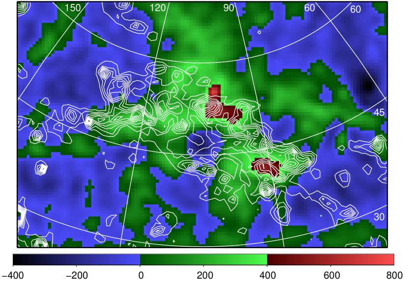
Figure 1.— Excess X-ray count rate in the region of Complex C. The excess is denoted by color, in units of $10^{-6}$ ROSAT 1/4 keV counts s^-1 arcmin^-2, and was calculated by subtracting a model which included smooth foreground and distant components from the observed ROSAT All Sky Survey count rate. The distant component of our subtracted background model experienced extinction by Galactic H I. Note that the plotted values are the observed excess count rates; they have not been de-absorbed. The white contours show the location of H I with velocity, $v<-90$ km s^-1. The contour spacing is $10^{19}$ cm^-2. Latitude is marked by the upward curving lines. They are spaced 15^o apart, with the lowest visible line marking $b=30^{\rm{o}}$. Longitude is marked by radiating lines. They are spaced 30^o apart, with the left-most visible line marking $l=150^{\rm{o}}$. The map shows that the brightest excess 1/4 keV count rates are aligned with Complex C and that the Complex C region is generally bright in soft X-rays.

Like Hirth et al. (1985), Bregman et al. (2009) suggested that the excess X-rays may have been emitted by shock-heated gas. Shock heating would be possible if the collision speed were multi-hundred km s^-1 and the gas were initially warm or hot. For unmagnetized warm plasmas, the post shock temperature would be $\sim 1\times 10^{6}$ K if the collision speed were $300$ km s^-1 (Shu, 1992). Such a speed may be achieved by Magellanic Stream clouds, given that the orbital velocity of the Magellanic Stream is $378\pm 18$ km s^-1 (Bland-Hawthorn et al., 2007). As is the case for most HVCs, the impact speed of Complex C is unknown. Most HVCs have line-of-sight velocities $\lesssim 300$ km s^-1, but their total velocities may be much larger than their line-of-sight velocities if the angles between the HVCs’ velocities and the lines-of-sight are large. This is the case for the Smith Cloud, whose total velocity has been calculated from the variation in line-of-sight velocity as a function of observing angle and other observables to be $\sim 300$ km s^-1, while its line-of-sight velocity is only $\sim 100$ km s^-1 (Lockman et al., 2008). In addition, an HVC’s currently observed velocity may be less than its velocity when it first encountered the Galaxy. We examine the X-ray productivity of gas shocked by fast clouds in this paper.

Turbulent mixing should also be considered. As the cloud passes through the ambient medium, shear instabilities develop at the contact surface. Gas on either side of the interface mixes, resulting in a zone of intermediate temperature, intermediate density gas. This logic has been used to explain high ions associated with HVCs (Tripp et al., 2003; Fox et al., 2004; Kwak, Henley & Shelton, 2011). In this paper, we also consider the possibility that some of the transition zone gas may be hot enough and dense enough to yield observable quantities of X-rays.

Other potential mechanisms include magnetic reconnection (Kerp et al., 1994; Zimmer et al., 1996, 1997; Kerp et al., 1999). As high velocity clouds move through the halo and thick disk, they should deform and compress the magnetic field. Zimmer et al. (1996, 1997) suggest that shear between the cloud and the ambient plasma will turbulently mix the magnetic field in the region very near to the cloud. When these magnetic field lines reconnect, they release energy. Zimmer et al. (1996, 1997) performed analytic and resistive magnetohydrodynamic simulations of the system finding that magnetic reconnections can release enough energy to heat the gas to $>10^{6}$ K. Because the magnetic reconnection scenario has already been examined with magnetohydrodynamic simulations, it is not simulated again in this paper. Recently, additional ideas have been suggested. Noting the X-rays emission that follows after charge exchange reactions in the heliosphere, Provornikova, Izmodenov, & Lallement (2011) suggest that charge exchange may be important at the interfaces between clouds and hot gas, and, noting the possible role of MHD plasma waves in heating the solar corona Jelínek & Hensler (2011) suggest that plasma waves instigated by collisions between high velocity clouds and halo gas may also be important.

In order to better understand HVCs, their interactions with the Galaxy, and the possibility that they may induce X-rays, we perform FLASH magnetohydrodynamic simulations of the shock heating and turbulent mixing scenarios. Our simulations begin with a cloud of similar size and H I column density as the lumps in Complex C. In our simulations of the shock heating scenario, the cloud initially has a speed of $\geq 200$ km s^-1 relative to the ambient gas. We examine the effect of ambient density, using moderate (e.g., $n\sim 7\times 10^{-3}$ atoms cm^-3) and lower densities for the ambient gas. The moderately dense ambient medium may represent material ablated from a preceding HVC or a thick disk/halo cloud. We found that when $\geq 300$ km s^-1 clouds interact with moderate density ambient media and radiative cooling is disabled, the shocked, compressed ambient medium yields extremely bright X-rays for $\sim 10$ Myr. If, in contrast, radiative cooling proceeds at the collisional ionizational equilibrium (CIE) rate, then the gas is only moderately bright and for only $\sim 1$ Myr. In both the adiabatic and the radiatively cooling simulations, greater ambient densities resulted in greater emission intensities. In our turbulent mixing simulations, a cool cloud falls through hot halo gas that is in hydrostatic equilibrium. In the simulations having very hot ambient media ($T=3\times 10^{6}$ K), the mixed zone contains some $T\sim 10^{6}$ K gas, which is hot enough to produce 1/4 keV X-rays in CIE calculations. However, the mixed gas falls behind the cloud, into a region where the pressure and density are low. It is the low density that limits the X-ray production of this scenario, causing the surface brightnesses to be too small to be detectable.

In Section 2, we describe the modeling algorithms and list the simulational parameters. Section 3 presents the results. In Section 3.1, we compare CIE and non-equilibrium ionization (NEI) calculations, finding that the CIE approximation yields similar 1/4 keV X-ray spectra to the NEI calculations. In Section 3.2, we evaluate the ability of fast HVC collisions to shock heat the ambient gas and induce X-ray emission. The predictions include 1/4 keV surface brightnesses, O VII and O VIII intensities, and O VII column densities. In Section 3.3, we evaluate the ability of turbulent mixing to create hot, X-ray emissive gas. Section 3.4 describes how the simulated clouds would appear to observers while Section 3.5 discusses higher and lower resolution simulations, concluding that the numerical resolutions used in our earlier simulations are adequate. The results are summarized in Section 4.

2. Modeling Technique

2.1. Magnetohydrodynamic Algorithms

We use similar hydrodynamic and magnetohydrodynamic algorithms as in Kwak, Shelton & Raley (2009); Kwak & Shelton (2010). To wit, we use the FLASH computer code, version 2.5 (Fryxell et al., 2000) with adaptive mesh refinement (AMR) to model the hydrodynamics and magnetohydrodynamics of fast moving clouds and ambient gas. For our suite of cloud shock simulations (Section 3.2), we test the effects of radiative cooling by modeling it in some simulations but not others. The radiative cooling calculations are done with the FLASH module, which uses cooling rates for CIE plasmas. We do not simulate gravity in our cloud shock simulations, but instead start the cloud with a large initial velocity. We do the same in our CIE testing (Section 3.1) and resolution experiments (Section 3.5). In our turbulent mixing simulations (Section 3.3) we use the gravity module in FLASH and the expression for gravitational acceleration presented in Ferrière (1998) to establish hydrostatic equilibrium in the background gas and to simulate the Milky Way’s gravitational pull on the cloud. In order to maintain hydrostatic balance in the background gas, radiative cooling must be disallowed and is so in the turbulent mixing simulations. It is not needed in the CIE testing and so is disabled in them as well. In two of our simulations, we model a magnetic field oriented perpendicular to the cloud’s motion. The others have no magnetic field. For the purposes of the magnetohydrodynamics, we treat all of the gas as if it is fully ionized in all of our simulations. Thermal conduction is not modeled.

The predictions of the X-ray count rates and very high ion column densities require predictions of the fractions of ions in any given state in the gas. We calculate the ion fractions using collisional ionizational equilibrium (CIE) and/or partially non-equilibrium ionization (NEI) models. In the CIE models, the ionization levels are calculated from the temperature of the simulated gas, using the Raymond and Smith code (Raymond & Smith (1977), with updates). For the NEI models, we enable FLASH to track the ionization levels of select elements as a function of time by accounting for their collisional ionization and recombination during each timestep. Ionization and recombination rates from Summers (1974) are used. We limit our NEI calculations to only two elements, silicon and oxygen, in order to economize on CPU and memory. Silicon is a major contributer to X-ray spectra in the 1/4 keV band, while oxygen is an important contributer in the 3/4 keV band. In Section 3.1, we show that CIE models adequately approximate the NEI models.

In our CIE tests (Section 3.1), shock heating analysis (Section 3.2), and turbulent mixing analysis (Sections 3.3), we use a 3 dimensional Cartesian coordinate system with width (span in the $x$ direction), and depth (span in the $y$ direction) of 1.5 kpc and 1.5 kpc, respectively. The footprint is centered on $x=0$ kpc, $y=0$ kpc. Most of these simulations use a domain that is 6 kpc tall. The exceptions are the high resolution, radiatively cooling, shock scenario simulations, for which we reduced the domain height to 1.5 kpc. In the turbulent mixing simulations, hydrostatic equilibrium is achieved by decreasing the thermal pressure with height above the midplane. We set the physical conditions at the base of the domain to simulate those in the ISM at $z=8$ kpc, thus in these simulations the domain runs from $z=8$ to 14 kpc. In the remaining simulations, there are no gravitational, density, pressure, or magnetic field gradients in the modeled ambient gas. Thus, an arbitrary $z$ offset can be added to the height along the $z$ axis. For these simulations, we choose to call the lower boundary $z$ = 0 kpc, only for convenience. In the shock models that had no radiative cooling, each domain is initially segmented into 4 blocks. Each block is subdivided by the AMR routine an additional 3 to 5 times, with the number of subdivisions depending upon the density gradient. With 5 levels of refinement, the resulting blocks are $1500/(2^{5-1})$ pc, on a side, while with 3 levels of refinement they are $1500/(2^{3-1})$ on a side. Each of these blocks is segmented into 8³ zones, which, consequently, range in size from (12 pc)³ to (47 pc)³. Like the shock models that had no cooling, some of our shock models that had cooling also had moderate resolution and 6 kpc tall domains initially made from 4 blocks, while others used higher resolution and a single 1.5 kpc tall block that was subdivided an additional 3 to 7 times depending upon the density gradient. These blocks were then subdivided into 8³ zones that range in size from (2.9 pc)³ to (47 pc)³. For our resolution tests (Section 3.5), we use both 3 dimensional Cartesian domains and 2 dimensional cylindrically symmetric domains and test maximum refinement levels between 4 and 8.

We calculate each zone’s emission spectrum using the Raymond and Smith spectral code (Raymond & Smith 1977, with updates), the gas density calculated by FLASH, the ionization levels from either the CIE or the NEI calculations, and Allen (1973) cosmic abundances. The Allen abundances are greater than the gas phase abundances in the halo and clouds. For example, the gas phase metal abundances in the warm halo are $\sim 4/10$ of the Allen solar abundances (Savage & Sembach, 1996), while the gas phase oxygen abundance in Complex C is about $\sim 1/10$ to $\sim 1/4$ of the Allen solar values (Fox et al., 2004), and the gas phase metal abundances in Magellanic Stream clouds are $\sim 1/14$ of the Allen solar values (Fox et al., 2010). The strength of the emitted spectra should be scaled accordingly, bearing in mind that in the shock scenario (the most X-ray productive scenario), the X-rays originate in the ambient gas and that over time, collisions in hot gas break down dust.

In order to obtain the spectrum pertaining to any given line-of-sight, we sum the spectra from the intersected zones. If the zones have differing sizes, we weight the terms accordingly. The X-ray spectra are convolved with the ROSAT response matrix in order to determine the count rate in the ROSAT R12 band, the 1/4 keV energy band. For the brighter models, we also report intensities at the photon energies of the O VII triplet ($\sim 570$ eV) and O VIII Lyman alpha line (653 eV). During our line intensity calculations, we do not subtract the continuum or the pseudo-continuum composed of faint, unresolved lines, because they account for $\sim 5\%$ of the emission in these energy bins during the brightest phases. They account for a greater fraction of the intensity when the gas is dimmer, but at these times, the reported intensity is too dim to be observed. In addition, for comparison with the observed X-ray excess associated with a Magellanic Stream cloud (Bregman et al. 2009; $0.64\pm 0.10$ counts ks^-1 arcmin^-2 seen by the XMM-Newton pn detector in 0.4 to 1.0 keV X-rays), we calculate the XMM pn count rate for four of our shock models.

We calculate the density of O VII ions for select models by combining the fraction of oxygen in the O VII ionization state with the oxygen abundance and the gas density in each zone. We integrate the density along sight lines through the domain in order to obtain O VII column densities. Again, the results can be scaled if elemental abundances other than those of Allen (1973) are preferred.

2.2. Cloud and ISM Parameters

We initialize the 6 kpc tall domains such that a spherical cloud is located in the upper portion of the grid and is surrounded by stationary ambient gas. In the 1.5 kpc tall domains, the center of the cloud is initially located at 2/3 of the height of the domain. At the beginning of each simulation, the cloud has a radius of 0.2 kpc, which corresponds to 1.1° if the cloud is seen from the current distance to Complex C (10 kpc; Thom et al. 2008). In most of our simulations, the cloud’s initial volume density of hydrogen nuclei, $n_{cl,H}$, is $0.0645$ cm^-3. Note that the simulations assume a 10 to 1 ratio of hydrogen to helium, making the mass density $0.0903$ amu cm^-3 and note that the number density shown in the figures and quoted in the text is the number of hydrogens per unit volume. We choose an initial hydrogen volume density of $0.0645$ cm^-3 because clouds with this density and a radius of 0.2 kpc have hydrogen column densities along sight lines through their centers of $8\times 10^{19}$ H cm^-2, which is similar to the observed H I column density in small features within Complex C. Initial cloud temperatures range from 100 K to $\sim 11,000$ K and are chosen from the constraint that the cloud’s initial thermal pressure must balance the initial thermal pressure of the gas around it. In our cases with magnetic fields, the initial magnetic field pressures also balance.

Table 1 lists the cloud and interstellar medium parameters for our simulations. They are grouped into three general cases, case A (clouds falling under the influence of gravity through a hot ambient medium that is in hydrostatic equilibrium; all of these test turbulent mixing, and some also test shock heating), case B (fast clouds moving through hot, rarefied gas before colliding with warm, moderate density ambient gas; these test shock heating and there are two categories, those with radiative cooling (Br) and those without (Ba)), and case C (fast clouds moving through warm, moderate density ambient gas; these test shock heating).

Table 1Simulation Parameters

Model	Comment	$n_{cl}$	$T_{cl}$	$n_{ISM}$	$T_{ISM}$	$v_{z}$	$B_{y}$
		(H cm-3)	(K)	(H cm-3)	(K)	(km s-1)	($\mu$G)
A1	note a	$6.45\times 10^{-2}$	$7.83\times 10^{2}$	see Figure 2:	$10^{6}$	$0$	0
A2	” $h=11$ kpc	”	”	”	”	$-50$	”
A3	note a	$6.45\times 10^{-3}$	$7.83\times 10^{3}$	”	”	$0$	”
A4	”	$6.45\times 10^{-2}$	$7.54\times 10^{3}$	”	$3\times 10^{6}$	”	”
A5	”	”	$1.11\times 10^{3}$	”	$10^{6}$	”	”
A6	”	”	$7.83\times 10^{2}$	”	”	”	0.1
A7	”	”	”	”	”	”	0.5
A8	”	”	$1.11\times 10^{3}$	”	”	$-300$	0
A9	”	”	”	”	”	$-400$	”
A10	”	$6.45\times 10^{-3}$	$1.11\times 10^{4}$	”	”	$-300$	”
A11	”	$0.15$	$4.6\times 10^{3}$	”	$3\times 10^{6}$	0	”
Ba2	notes b and ba	$6.45\times 10^{-2}$	$10^{3}$	$6.45\times 10^{-3}$	$10^{4}$	$-200$	”
Ba3	”	”	”	”	”	$-300$	”
Ba4	”	”	”	”	”	$-400$	”
Ba5	”	”	”	”	”	$-500$	”
Ba6	”	”	”	”	”	$-600$	”
Br2	notes b and br	”	”	”	”	$-200$	”
Br3	”	”	”	”	”	$-300$	”
Br4	”	”	”	”	”	$-400$	”
Br3d	”	”	$10^{2}$	$6.45\times 10^{-4}$	”	$-300$	”
C3	note c	”	$10^{3}$	$6.45\times 10^{-3}$	”	$-300$	”
C4	”	”	”	”	”	$-400$	”
C5	”	”	”	”	”	$-500$	”
C6	”	”	”	”	”	$-600$	”
C3d	”	”	$10^{2}$	$6.45\times 10^{-4}$	”	$-300$	”
C6d	”	”	”	”	”	$-600$	”

Note. —

note a: Unless otherwise stated, the clouds in the suite A models begin at height $h=12$ kpc. The temperature at the cloud’s initial center is listed, but the cloud’s temperature varies slightly with height in order to balance the cloud’s pressure with that of the ambient gas. In models A1 through A11, the thermal pressures at the midplane are 6000, 6000, 6000, 4190, 8480, 6000, 6000, 8480, 8480, 8480, and 5930 K cm^-3, respectively. All suite A simulations assume CIE ionization levels and no radiative cooling.

note b: The tabulated temperature and density refer to those of the warm ISM; the hot ISM, occupying the upper 1.5 kpc (in the Model Ba simulations) or 1.0 kpc (in the Model Br simulations) of the domain has a temperature of $10^{6}$ K and a density of 1/100 of that in the warm ISM.

note ba: All suite Ba simulations assume CIE ionization levels and no radiative cooling.

note br: All suite Br simulations modeled NEI ionization fractions for select elements during their FLASH runs and CIE ionization fractions in the post processing. In addition all Br simulations include radiative cooling. We made both moderate and high resolution versions of the Model Br simulations.

note c: All suite C simulations assume CIE ionization levels and no radiative cooling.

In our suite of case A simulations, the ambient medium is either $T_{ISM}=1\times 10^{6}$ or $3\times 10^{6}$ K and, as mentioned in Subsection 2.1, radiative cooling is disabled in order to maintain hydrostatic equilibrium in the ambient gas. We determine the initial density gradient from the equation for hydrostatic equilibrium with the constraints that the magnetic field strength and temperature are constant. We constrain the midplane density by requiring the midplane thermal pressure to be reasonable, i.e. roughly 6000 K cm^-3, and the 1/4 keV X-ray surface brightness of the ambient medium above $z=2$ kpc to be comparable to observationally derived values. As an example, we note the X-ray surface brightness in the 1/4 keV ROSAT band produced by the gas above 2 kpc in our Model A reference run, A1. Its intrinsic surface brightness is $1510\times 10^{-6}$ counts s^-1 arcmin^-2. If the column density of intervening H I is $1\times 10^{20}$ cm^-2, then the absorbed surface brightness is $583\times 10^{-6}$ counts s^-1 arcmin^-2, which is consistent with measurements presented in Snowden et al. (1998, 2000). Our constraints yield the ambient density functions plotted in Figure 2; thus the density of ambient gas, expressed in units of hydrogens per unit volume, at the cloud’s initial height in most of our Case A simulations is between $\sim 5\times 10^{-5}$ and $2.5\times 10^{-4}$ cm^-3. The values are consistent with those used or determined elsewhere (e.g., density of $\gtrsim 2.4\times 10^{-5}$ cm^-3, (Blitz & Robishaw 2000, ram pressure stripping of nearby dwarf galaxies); $\sim 5\times 10^{-5}$ cm^-3, (Moore & Davis 1994, ram pressure stripping of Magellanic Clouds); $2\times 10^{-4}$ cm^-3 in model by Bland-Hawthorn et al. (2007); 1 and $3\times 10^{-4}$ cm^-3 in models by Heitsch & Putman (2009)). In order to balance the ambient and cloud pressures at the beginning of each simulation, we allow the cloud temperature to vary slightly with height. We make a suite of simulations in order to sample various initial cloud heights and velocities, ambient densities and temperatures, and strengths of the magnetic field lying parallel to the Galactic midplane. All of the Case A models use CIE calculations in order to determine the fraction of atoms in any given ionization state. The hydrodynamical results from Model A are stored at 2 Myr intervals.

Figure 2.— Density of ambient gas, expressed in units of hydrogen atoms per cm^-3, as a function of height above the Galactic plane for the models that have hydrostatic environments, i.e., Models A1 through A11.

In our suite of Case B simulations, the clouds pass through a hot ambient medium before hitting a warm extended medium. The hot medium may represent halo or intergalactic gas, while the warm medium may represent material shed from a preceding HVC, a high $z$ cloud, or, given the proximity of some HVCs to the Galactic disk, it may represent warm gas in the Galaxy’s thick disk. In our set-up, the hot and warm sectors are in pressure balance with each other. In most of our Model B simulations, the hot medium has a temperature of $T_{ISM}=1\times 10^{6}$ K, density of hydrogen of $n_{ISM,H}=6.45\times 10^{-5}$ cm^-3, i.e. $n_{cl,H}/1000$, and occupies the uppermost 1.5 kpc of the grid. The density of the hot portion of the domain is equal to that at $z\sim 12$ kpc in Models A1, 2, 3, 6, and 7. In most of our Model B simulations, the warm part of the domain has a temperature of $T_{ISM}=10^{4}$ K, density of hydrogen of $n_{ISM,H}=6.45\times 10^{-3}$ cm^-3, i.e. $n_{cl,H}/10$, and occupies the lower 4.5 kpc of the grid. At the beginning of each Case B simulation, the environmental gas is in pressure balance with the cloud. There is no magnetic field and therefore no magnetic pressure. It is not practical to model hydrostatic equilibrium in Case B because the weight of the warm medium cannot be supported unless the pressure has a strong gradient. By giving up hydrostatic equilibrium, we also give up gravity. Because both are absent, an arbitrary offset can be added to our domain’s $z$ without affecting the results. On this arbitrary scale, the initial location of the center of the cloud is $z=5$ kpc in simulations having 6 kpc tall domains (the moderate resolution simulations) and 0.5 kpc from the top in the simulations having 1.5 kpc tall domains (the high resolution simulations). Lacking gravity to accelerate them, the clouds must be given an initial velocity. We sample several velocities; see Table 1. Cases with speeds of 200 and 300 km s^-1 can be used for some Galactic HVCs. Cases with speeds of 300 and 400 km s^-1 can be compared with the Magellanic Stream, whose orbital speed is $378\pm 18$ km s^-1 (Bland-Hawthorn et al., 2007). The simulations with faster clouds are useful for identifying trends. We test the effects of non-equilibrium ionization(NEI) by creating a small suite of models and for which both NEI and CIE ionization fractions are calculated (these models have names that begin with Br and include radiative cooling). We test the effects of radiative cooling at the CIE rate by comparing models with and without radiative cooling. Those without radiative cooling have names that begin with Ba. The computational results for Case Ba models are stored at 2 Myr intervals. We performed several Model Br simulations with the same resolution and archival time intervals as the Model Ba simulations, but in order to better model the radiative cooling in this scenario, simulations having smaller zone sizes and stored time intervals are also needed. Thus, we also present simulations of Br models in which up to 7 levels of refinement are allowed, the spacing between archived epochs is 40,000 years, and the simulations are stopped at 2 Myr. It is this set of simulations that has 1.5 kpc domain heights.

Case C is a variation on Case B, with the primary difference being that all of the ambient gas is warm ($T_{ISM}=1\times 10^{4}$ K) in Case C. In Case C, we also sample two ambient densities, a rarefied case having $n_{ISM,H}=6.45\times 10^{-4}$ H cm^-3 and a moderate case having the same density as the warm gas in Case B, i.e. $n_{ISM,H}=6.45\times 10^{-3}$ H cm^-3. In the former case, we also reduce the clouds’ temperature in order to achieve pressure balance at the beginning of the simulations. All of the Case C models use CIE calculations, omit radiative cooling, and are archived every 2 Myr.

3. Results

3.1. Validity of CIE Approximation

In order to evaluate the CIE approximation, we compare spectra that we calculate from the NEI and CIE ionization fractions of silicon and oxygen. The NEI ionization fractions, i.e., the fractions of the atoms at any given ionization level were obtained by having FLASH track the ionization levels in a time dependent fashion in moderate resolution versions of models Br3, Br4, and Br5. The CIE ionization fractions were obtained from the hydrodynamic information for these same models; specifically, they were calculated by the Raymond and Smith code using the temperature of the gas as an input. For each of these three models, we calculate the spectra produced by NEI silicon, CIE silicon, NEI oxygen, and CIE oxygen for various vertical sight lines through the domain at each epoch, 2 Myr, 4 Myr, etc. (Although the shocked gas has already radiated way much of its energy by 2 Myr, it is still sufficiently emissive for these experiments.) In order to reduce the quantity of information, we then convolve each silicon spectrum with the ROSAT 1/4 keV band response function and each oxygen spectrum with the ROSAT 3/4 keV band response function, yielding count rates in these bands. In each case, the CIE count rates in the 1/4 keV band are fairly similar to the NEI count rates. For example, the ROSAT 1/4 keV count rate calculated from the CIE and NEI silicon spectra produced along the central sight line of the Br4 model at 2 Myr are within $5\%$ of each other. The relationship between the CIE and NEI oxygen spectra were not as consistent from model to model and epoch to epoch. For Model Br4 at 2 Myr the CIE and NEI oxygen spectra are within $14\%$ of each other. The emission line spectra for this case are displayed in Figure 3. Sometimes, the O VII intensities from the models are less consistently aligned with each other than are the silicon intensities and frequently the O VIII quantities (which are always small) are poorly aligned, presumably due to delayed ionization and recombination. Similarly, the high resolution Model Br simulations also show poor alignment between the CIE and NEI O VIII column densities.

Figure 3.— Top: The emission line spectra of silicon, calculated using the NEI algorithm and the CIE algorithm, produced along the central sight line in the moderate resolution Br4 model at 2 Myr age. Bottom: The NEI and CIE emission line spectra produced by oxygen ions along the same sight line. This plot shows the similarity between the CIE and NEI spectra from silicon and oxygen, important contributers to the 1/4 keV and 3/4 keV count rates, respectively.

3.2. Shock Heating

Theoretically, if the clouds collide with neighboring gas at fast enough speeds, then shocks should develop in both media. The temperature ($T_{2}$) of the shocked plasma can be estimated from the equation for plane parallel shocks (Shu, 1992):

$$T_{2}=T_{1}\frac{[(\gamma+1)+2\gamma(M_{1}^{2}-1))][(\gamma+1)+(\gamma-1)(M_{1}^{2}-1)]}{(\gamma+1)^{2}M_{1}^{2}},$$ (1)

where $T_{1}$ is the temperature of the unshocked gas, $M_{1}$ is the Mach number calculated from the speed at which the unshocked gas is overrun by the shock, and $\gamma$ is the adiabatic constant for monotonic gas ($5/3$). Here, we compare the theoretical post-shock temperature with those of Models Ba3 and C3 at the first epoch ($t=2$ Myr). These models begin with cloud velocities of $v_{z}=-300$ km s^-1 and do not model radiative cooling (although, in post-processing, we can estimate the X-ray spectra that would be emitted by gas at the simulated temperatures). By the first archived epoch at 2 Myr of simulated time, the cloud has shock-heated the environmental gas beneath it while a reverse shock has been driven into the lower part of the cloud. In both Model Ba3 and C3, the shocked environmental gas was initially warm ($T=1\times 10^{4}$ K), ionized ISM. Although the unshocked portion of the cloud still travels with approximately its initial velocity, $v_{z}=-300$ km s^-1, at this epoch, the shocked portion of the cloud moves downwards at speeds between 240 and 300 km s^-1 and the swept up ISM moves downwards at speeds up to 240 km s^-1 with an average of about 200 km s^-1 and moves sideways with speeds exceeding 100 km s^-1. Thus, the impacted material does not simply pile up in front of the cloud, as in a shock-tube simulation, but instead partially skirts around the cloud. The shockfront travels downwards at 4/3 of the shocked ISM’s downwards speed, which is confirmed by the displacement of the shockfront between $t=2$ and 4 Myr. Thus, $M_{1}=18$. From equation 1, we find that $T_{2}$ should be $1.0\times 10^{6}$ K, which is consistent with the post-shock temperatures in Models Ba3 and C3: 0.95 and $1.0\times 10^{6}$ K, respectively. See Figure 4. Since the clouds decelerate in our gravity-less simulations, the post-shock velocity decreases with time and thus the post-shock temperature decreases with time as well. This can be seen by comparing the temperatures at 10 Myr with those at 2 Myr in Figure 4.

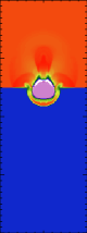
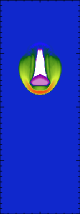
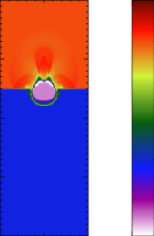
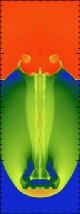
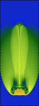
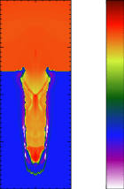
Figure 4.— The log of the temperatures of the cloud and ambient gas along a vertical slice through the centers of models Ba3, C3, and Br3 (left to right) at 2 Myr (top row) and at 10 Myr (bottom row). The color bars are keyed to the log of the temperature. The cloud appears at $z\sim 4.5$ kpc in the top images and at $z=2.6$ kpc in the bottom images. Only the upper 4 kpc of the domains are shown. The temperature elevations that resulted from the forward shock in the ambient gas and the reverse shock in the cloud can be seen in the Ba3 and C3 images. In contrast, the Br3 image shows little hot gas beneath the cloud, owing to radiative energy losses. In order to show the late-time evolution for Model Br3, we used our moderate resolution simulations. The apparent pixelation in the images is an artifact of the image processing and does not represent the resolution of the simulations.

A reverse shock propagates through the cloud, but due to the density contrast, it propagates slower than the forward shock in the ISM. In our simulations of model C3 at 2 Myr, the reverse shock moves into the cloud at a speed of $\sim 90$ km s^-1 from the cloud’s reference frame. Given an initial cloud temperature of $T_{cl}=1000$ K, the reverse shock should be strong and according to Equation 1, it should heat the cloud to $\sim 1.2\times 10^{5}$ K. Our simulational results find the temperature to range from the cloud temperature to this value; see Figure 4. While the reverse shock-heated material is far hotter than the unshocked portion of the cloud, it is still not hot enough to produce X-rays. The X-rays that result from this geometry originate in the shock-heated ambient medium. In the following subsections, we explain that their intensity ranges from unobservably dim to significantly bright, depending upon the time since interaction, collision speed, and strength of radiative cooling.

3.2.1 Effect of Radiative Cooling

The simulations and theory discussed above did not include the effects of radiative cooling. When it is included in the calculations, the shocked ambient gas quickly cools. This can be seen by comparing the temperature and density distributions in Models Ba3 and C3 with those from Model Br3 in Figure 4. These are fair comparisons because each model has the same parameters for the cloud and lower ISM and, although the ionization fractions of some elements were calculated in a time-dependent manner in Model Br3 (but not in the others), the NEI ionization levels did not affect the hydrodynamics and we replace them with the CIE ionization levels for the following spectral calculations. Furthermore, we note that the ambient medium in Models Ba3 and Br3 include a layer of hot gas, but this layer contributes only $1\times 10^{-6}$ counts s^-1 arcmin^-2 which is trivially small and is subtracted before we report the results.

Without radiative cooling, the shock-heated gas is very bright for millions of years. As can be seen in Figure 5, even the moderately fast clouds ($v_{z}=200$ km s^-1) induce surface brightnesses across their footprints of $\sim 1000$ $\times 10^{-6}$ counts s^-1 arcmin^-2 in the ROSAT R12 band at their peak. Faster clouds produce $\gtrsim 10,000\times 10^{-6}$ counts s^-1 arcmin^-2 in this band at their peaks. These models are much brighter than the typical intrinsic intensity of 1/4 keV photons emitted above the Galactic disk, which is $\sim 1000$ to $\sim 2000\times 10^{-6}$ counts s^-1 arcmin^-2 with significant directional variation (Snowden et al., 2000). All of these simulated clouds continue to make $>100\times 10^{-6}$ counts s^-1 arcmin^-2 until at least 14 Myr after the collision.

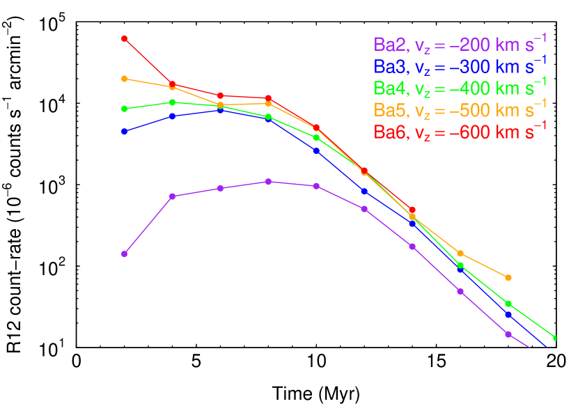
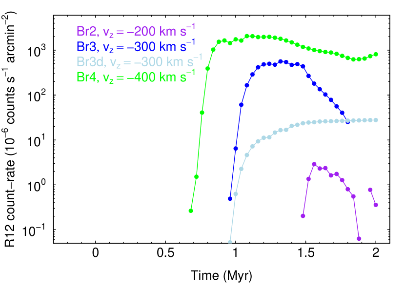
Figure 5.— Surface brightnesses in the ROSAT 1/4 keV band from Models Ba2, Ba3, Ba4, Ba5, and Ba6 and the high resolution versions of Br2, Br3, Br3d, and Br4 as functions of time. The surface brightnesses are averaged across a disk of radius 200 pc and given in units of $10^{-6}$ ROSAT 1/4 keV counts s^-1 arcmin^-2. The contribution made by undisturbed hot, background gas in the domain has been subtracted in order to obtain the reported results. The expected intensity due to the background gas is brighter than the emission in Model Br2 at $t=1.9$ Myr, resulting in unplotted negative count rates at that time. Due to their similarity with the case Ba models, the case C models are not shown.

When radiative cooling is included in the simulation, the hot gas in front of the cloud sheds most of its energy via radiation, only some of which is in the X-ray band. Figures 5 and 6 include plots of the resulting 1/4 keV surface brightnesses from the high resolution Model Br simulations. The average surface brightnesses across footprints that are 200 pc in radius peak around 3,  500, and $2000\times 10^{-6}$ counts s^-1 arcmin^-2 in the ROSAT 1/4 keV band within 1 to 1$\text@frac{1}{2}$ Myr of the collision for the $v_{z}=200,300$ and $400$ km s^-1 collisions, respectively.

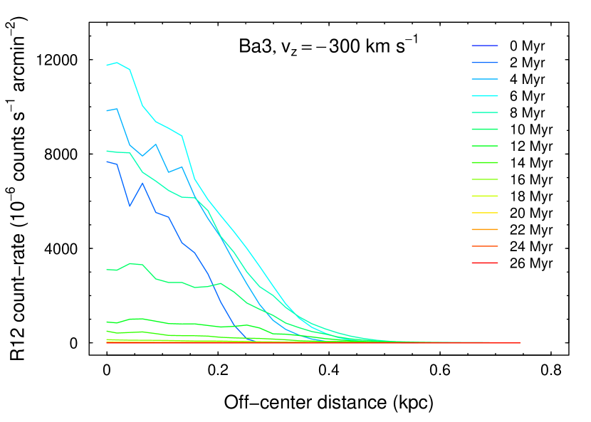
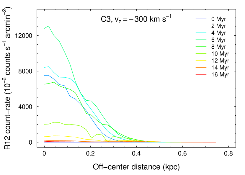
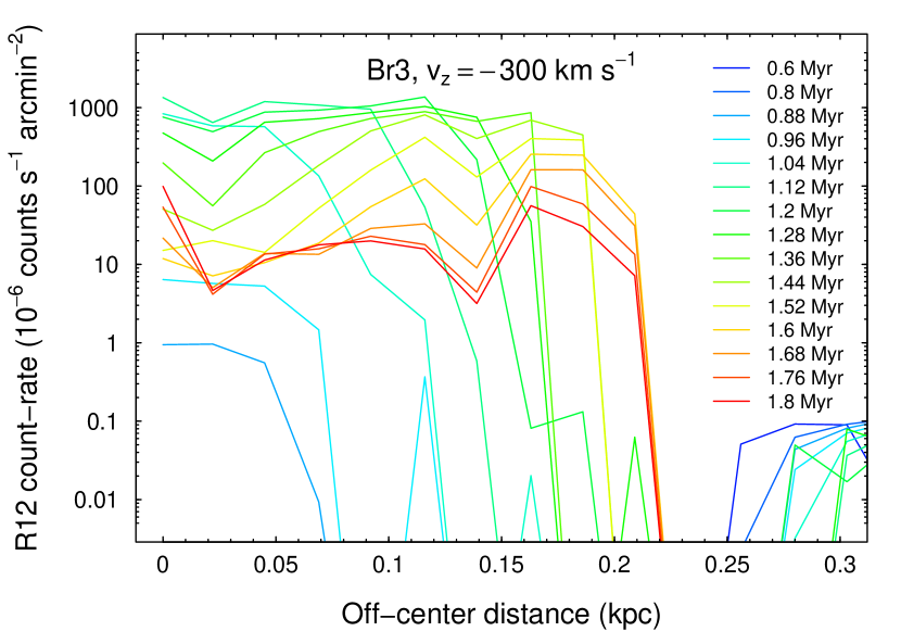
Figure 6.— X-ray count rates due to the shock produced by the fast-moving infalling clouds in Model Ba3 (top panel), Model C3 (middle panel), and the higher resolution Model Br3 (bottom panel). The ROSAT R12 count rate, i.e. the count rate in the 1/4 keV band, was calculated for vertical sight lines through the computational domain and is plotted relative to the distance from the projected center of the cloud. The background count rate has been subtracted from all of the plots. Results for Models C and Ba are shown at 2 Myr intervals until the clouds reach the bottom of their computational domains. The time granularity between stored epochs is much smaller for the higher resolution Br model and dimmer epochs at the beginning and end of the simulation are not shown.

The surface brightness profiles of Models Ba3 and C3 in Figure 6 show that the surface brightness peaks near each cloud’s axis and drops non-monotonically with radius. Model Br3’s profile is more complicated. The peaks and valleys in the profiles are associated with the density and temperature structure of the off-axis gas. When the gas is very bright, the profile extends beyond the footprint of the cloud. Sensitive X-ray observations of the clouds would see extended disks.

The shock-heated gas is less conspicuous in the 3/4 keV band than in the 1/4 keV band, in both the radiative cooling and the non-cooling scenarios. For both Models Ba3 and C3, the O VII triplet (photon energy $\sim 570$ eV) intensity across a disk of radius = 200 pc averages to $\sim 1$ photon s^-1 cm^-2 sr^-1 for the first several million years (see Figure 7). It averages to far less than 1 photon s^-1 cm^-2 sr^-1 for Model Br3. The former intensity is about $\sim 1/5$ of the typical observed intensity on randomly chosen sight lines away from the Galactic center (Henley & Shelton, 2010). Because the collisions weaken with time, the O VII intensities fade sooner than the 1/4 keV surface brightnesses. Furthermore, none of the $v_{z}=-300$ km s^-1 models produce appreciable O VIII intensities at any time.

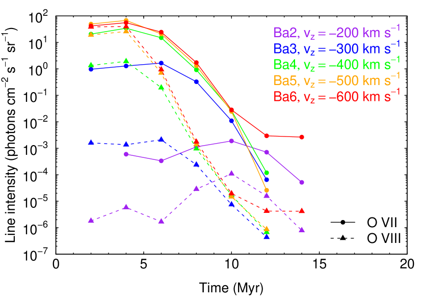
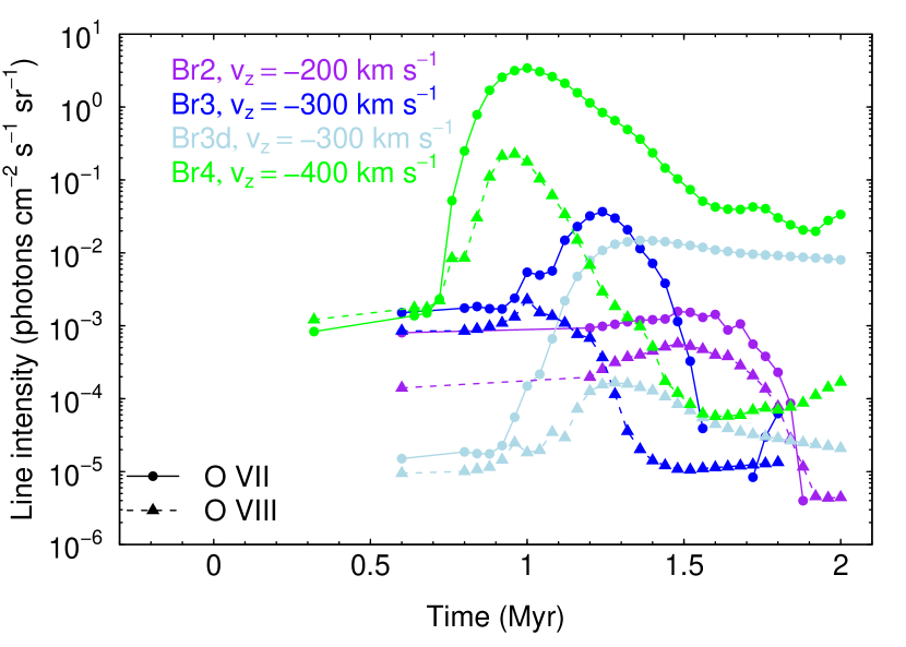
Figure 7.— The O VII and O VIII intensities as functions of time for Models Ba2, Ba3, Ba4, Ba5, and Ba6 (top) and the high resolution versions of Models Br2, Br3, Br3d, and Br4 (bottom). The intensities are given in photon units (photon s^-1 cm^-2 sr^-1) and averaged across a disk of radius 200 pc. The Case C models are not shown, but are roughly similar in brightness to the Case Ba models. As can be seen by comparing the top and bottom panels, the Model Ba peak intensities are roughly an order of magnitude brighter than the Model Br peak intensities.

The average O VII column density within a footprint of radius 200 pc is $3\times 10^{15}$ cm^-2, for both Models Ba3 and C3 at 2 Myr. It remains near this level for 10 Myr, thus outliving the duration of the bright O VII emission. In Model Br3, the average O VII column density is $\sim 4\times 10^{14}$ cm^-2 from about 1.3 to about 1.5 Myr. The O VII and O VIII column densities for these and other speeds simulated for Model Ba and the high resolution versions of Model Br are plotted in Figure 8.

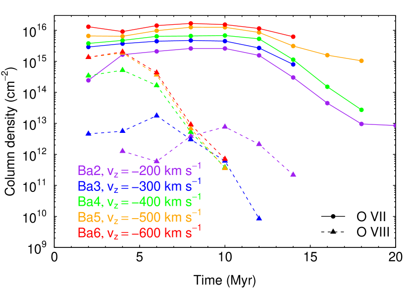
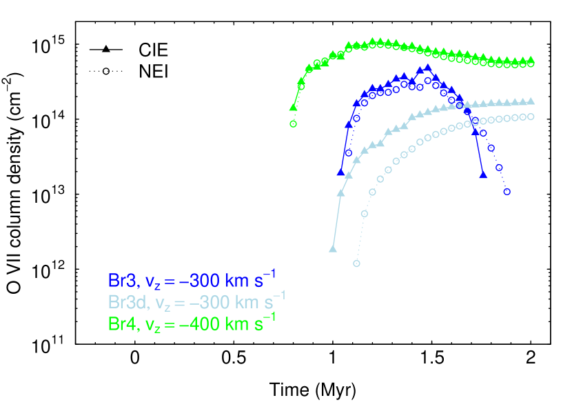
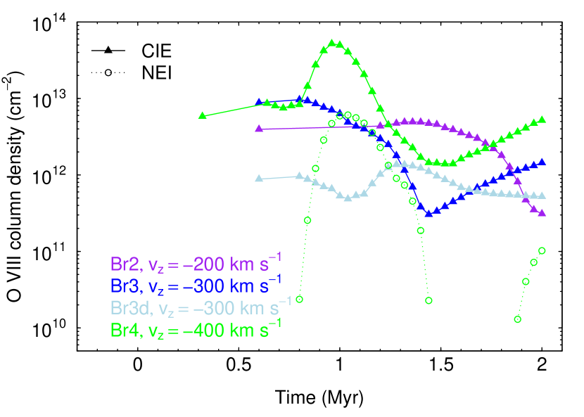
Figure 8.— Excess O VII and O VIII column densities as a function of time for Model Ba simulations and for high resolution versions of Model Br simulations. The hot ambient gas at the top of the simulational domain produces a background O VII column density of $1.94\times 10^{14}$ cm^-2 which has been subtracted and so does not contribute to the plotted values. The background-subtracted column densities have been averaged over disks of radius 200 pc in order to obtain the plotted values. For the Br models, we provide two predictions. The dashed lines mark the column densities calculated using the CIE approximation while the dotted lines mark the column densities obtained from NEI calculations done in FLASH. This plot demonstrates that the O VII column densities are greater for faster cloud speeds, greater when radiative cooling is not allowed, and remain high later than the O VII intensities.

The gas in these models is also UV emissive. When we divide the predicted energy spectra into 0.25-dex wide bins, we find that the 10 to 18 eV photon energy range is the most luminous part of the $\sim 5$ to $\sim 2000$ eV spectrum for Models Ba3, Br3, and C3. Model Br3, for example, radiates more than 100 times more power in 10 to 18 eV photons than in 100 to 180 eV photons when it is at its peak 1/4 keV X-ray brightness (age $\sim$1.3 Myr). At earlier and later times, the ratio is even larger. With its comparatively large radiative power, the UV plays a more important role in cooling the shock-heated gas than does the X-ray.

We have presented results for both radiatively cooling and adiabatic models. In the following subsections, we continue to discuss both cases. While, on the face of it, it appears contradictory to consider the X-ray count rates expected from hot gas whose hydrodynamics were calculated in models that excluded radiative cooling (Models Ba and C), we note that 1.) the true cooling rate is unknown, 2.) if the gas phase abundances are between zero and the solar values, then the cooling rate should be between that used in the Br suite of models and those used in the Ba and C suites, and 3.) X-ray emission accounts for very little cooling. Because X-ray emission accounts for such a small fraction of the cooling and because the relative contribution to the spectrum made by any given element varies from one energy band to the next, it is possible for variations in gas phase metallicities to preferentially lower the cooling rate compared with those in Case Ba or raise the X-ray count rate compared with those from Case Br. Iron provides a good example of the effect of the gas-phase metallicity. Almost $60\%$ of the energy radiated in 5 to 100 eV photons by a $T=10^{6}$ K plasma having Allen (1973) abundances are emitted by iron ions, while slightly less than $20\%$ of the ROSAT R12 counts are due to photons emitted by these ions. Thus, if the true iron abundance in the shock-heated gas were half that expected by Allen (1973), then the overall radiative cooling rate would be noticeably affected (it would be about $70\%$ of the CIE rate), while the ROSAT R12 count rate would be insignificantly affected (it would be about $90\%$ of CIE rate). Reducing the iron abundance to zero decreases the radiative cooling rate by 3/5, while reducing the 1/4 keV luminosity by only 1/5. Similar phenomena occur at higher temperatures. Silicon provides another example, because it accounts for $13\%$ of the 5 to 100 eV power, but almost $30\%$ of the ROSAT R12 count rate. Thus, doubling its relative abundance would increase the radiative loss rate by only 1/8, but increase the 1/4 keV count rate by almost third. Here, we aren’t suggesting that the halo has supersolar abundances of silicon, but are pointing out that if the ratio of silicon to other elements is larger than in solar abundance gas, the effect would preferentially benefit the X-ray luminosity. The interested reader is referred to Sutherland & Dopita (1993) figure 18 for relative cooling rates from various elements. Other reasons why the rate of radiative cooling might differ from the CIE rate for solar abundances include disequilibrium between electron and ion temperatures and delayed ionization and recombination.

3.2.2 Effect of HVC Velocity

We ran several additional simulations in order to explore the effects of initial velocities. These, plus the simulations already mentioned, create several suites. Models Ba2, 3, 4, 5, and 6 have initial cloud velocities of $v_{z}=-200,-300,-400,-500$, and $-600$ km s^-1, respectively. Models C3, 4, 5, and 6 have velocities of $v_{z}=-300,-400,-500$, and $-600$ km s^-1, respectively. The faster end of this range is greater than expected for HVCs near our galaxy, but may be of value for studying more energetic collisions. Models Br2, 3, and 4 have velocities of $v_{z}=-200,-300$, and $-400$ km s^-1, respectively. We simulated the Model Br suite in both moderate and high resolution forms, but for this analysis, we focus on only the high resolution simulations.

Even the $v_{z}=-200$ km s^-1 cloud induces bright X-rays in the non radiatively cooled simulations and some X-rays in the radiatively cooled simulations. These X-rays are from gas that was shock-heated to $T\sim 5\times 10^{5}$ K. The faster clouds shock-heat the ISM to higher temperatures. As a result, they produce more 1/4 keV X-rays for longer periods of time (see Figure 5). Furthermore, the O VII and O VIII intensities, which are modest in models Ba2 and Ba3, become stronger in Models Ba4, 5, and 6 (see Figure 7). Because the shock heated gas is more highly ionized in the faster models, the column densities of O VII and O VIII are also larger (see Figure 8).

3.2.3 Effect of Density

The density of the environmental gas affects the hydrodynamics and production of 1/4 keV X-rays in multiple ways. When the ambient density is greater, then the swept up, shock-heated environmental gas in front of the cloud has greater density and depth, resulting in a higher 1/4 keV surface brightness. In addition, denser gas better decelerates the cloud, resulting in lower post-shock temperatures. The effect of lowering the post-shock temperature, however, can increase or decrease the emissivity, depending upon the circumstances. Given that the peak in the theoretical 1/4 keV X-ray emissivity curve is near $T=0.9\times 10^{6}$ K for CIE plasmas, slowing the cloud increases the 1/4 keV X-ray emissivity in the cases of very fast clouds (e.g., those with initial $v_{z}=-600$ km s^-1) and decreases it in the cases of only moderately fast clouds (e.g., those that have reached $v_{z}=-250$ km s^-1.) With each of these factors playing a role, our Model C3 is 10 times brighter than its less dense counterpart, Model C3d, whose environmental density is 1/10 that of Model C3. Our Model C6 is 100 times brighter than its less dense counterpart, Model C6d, whose environmental density is 1/10 that of Model C6, and our Model Br3 is $\sim 30$ times brighter than its less dense counterpart, Model Br3d, whose environmental density is 1/10 that of Model Br3. Furthermore, the greater the amount of shock-heated interstellar material that is swept up, the greater the column densities of very high ions. Consequently, Models C3 and C6 have about 10 times greater O VII column densities than Models C3d and C6d, respectively, while Model Br3 has roughly twice the O VII column densities of Model Br3d.

3.3. Turbulent Mixing

Here, we consider mixing between cool and warm clouds as they travel through hot, rarefied ambient gas. As the cloud passes through the hot gas, Kelvin-Helmholtz instabilities develop and mixing between the cloud and ambient material creates a zone of intermediate temperature, intermediate density gas (Esquivel et al., 2006). Analytical calculations and computational simulations have already shown that mixed layers are rich in high ions, such as O VI (Slavin et al., 1993; Esquivel et al., 2006; Kwak & Shelton, 2010; Kwak, Henley & Shelton, 2011). In order to determine whether or not mixing zones between HVCs and very hot gas can also be X-ray productive, we simulate the hydrodynamics of 3 dimensional clouds passing through hot, rarefied gas. This approach differs from the more common approach, which treats the two regions as blocks that slide past each other, but better replicates the effects of the cloud’s rounded shape and motion. The names of these simulations begin with A.

In order to model the interaction adequately, the simulations must resolve the mixing length scale. Interstellar turbulence may exist across a wide range of length scales, but the largest length scale dominates the mixing (Esquivel et al., 2006). In our case, the largest length scale is the height of the distorted cloud. This height and width are adequately resolved in our Model A simulations, which, when fully resolved, use $\sim 30$ zones to model a 400 pc span (the nominal height of the interaction zone in Figure 9).

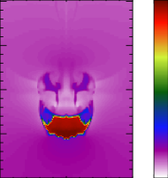
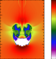
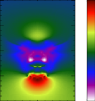
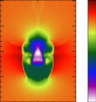
Figure 9.— Number density of hydrogen atoms (top left), temperature (top right), pressure (bottom left), and velocity in the $z$ direction (bottom right) of the A11 cloud and the material ablated from it after the cloud has fallen for 30 Myr through hot halo gas. The density plot is logarithmic, while the others are linear. The images show a vertical slice through the center of the cloud at $x=0$ kpc. The ablated and mixed material appear to form ears on the sides of the cloud in the top two figures. Because of the symmetry in the initial conditions, the trailing stream of dislodged gas actually forms a crown shape. The pressure behind (i.e., above) the cloud is noticeably low. The apparent pixelation is an artifact of the image processing and does not represent the resolution of the simulations.

Our simulations do not include thermal conduction, but de Avillez & Breitschwerdt (2007) found that turbulent diffusion is much more effective than thermal conduction at leveling the temperature gradient. Thus, our omission of thermal conduction is not problematic. Note, also, that radiative cooling has not been allowed in the Model A simulations. It was disallowed in order to maintain hydrostatic balance in the background gas. The ramifications of cooling are too complicated for us to simply say that adding cooling would lower the radiation rates of the turbulently mixed gas. This is because radiative cooling would not only allow the $\sim 1\times 10^{6}$ K gas to cool to lower temperatures, but it would allow hotter gas to cool to $\sim 1\times 10^{6}$ K.

Model A1 serves as an example of Case A simulations and as our reference simulation for comparison with the others. In this simulation, we track the cloud as it falls from its initial height of 12 kpc to near the bottom of our grid ($z=8$ kpc), which takes 32 Myr of simulated time. We record the simulation results at 2 Myr intervals and here describe the results at two of the sampled epochs. By 16 Myr, the cloud has accelerated to $v_{z}=-120$ km s^-1 and fallen to a height of $z\sim 11$ kpc. By 30 Myr, it has accelerated to $v_{z}=-220$ km s^-1 and fallen to $z\sim 8.2$ kpc. We obtain the cloud-induced excess intrinsic count rate in the 1/4 keV band by subtracting the count rate of the undisturbed hot halo from that toward the disturbed gas. Vertical sight lines throughout the domain are sampled. At 16 Myr, the brightest X-ray excess is $0.1\times 10^{-6}$ counts s^-1 arcmin^-2. At 30 Myr, it is $0.4\times 10^{-6}$ counts s^-1 arcmin^-2. The latter is the brightest rate for Model A1 at any time. Note that these are intrinsic count rates; absorption by $N_{H}\sim 10^{20}$ cm^-2 would decrease them by factors of $>2$. Even without absorption, the small count rate enhancements would be inconspicuous against the diffuse X-ray background.

The timescale for the growth of the Kelvin-Helmholtz instabilities decreases as the cloud falls and the density contrast between the cloud and the ambient gas decreases. For the last $\sim 14$ Myr of the simulation, we estimate that the timescale for the growth of instabilities is $\lesssim 14$ Myr, from Chandrasekhar (1961) Section 101, and assuming that instabilities grow on similar timescales in plane parallel geometries as in our geometry. Hence, the lack of X-rays due to turbulent mixing in our simulations is unlikely to be due to the instabilities having insufficient time to grow.

Models that simulate a larger ambient temperature (Models A4 and A11), a greater ambient pressure (Models A5 and A11), faster initial speeds (Models A2, A8, A9, and A10), denser clouds (Model A11), less dense clouds (Models A3 and A10), and nonzero magnetic fields (Models A6 and A7) were also simulated. Of the slow models (initial $|v_{z}|\leq 50$ km s^-1) the greatest X-ray enhancement seen anywhere in the domain at any time during the simulations is $35\times 10^{-6}$ counts s^-1 arcmin^-2. This occurred in Model A11 at 30 Myr, just before the cloud crossed the domain’s lower boundary. The next brightest model was Model A4, with a peak enhancement of $14\times 10^{-6}$ counts s^-1 arcmin^-2 at 30 Myr, also just before the cloud crossed the domain’s lower boundary. Models A4 and 11 have the largest ambient gas temperature ($T_{ISM}=3\times 10^{6}$ K) and, through most of the domain, have the largest ambient density of all of the Case A models. These attributes prime Models A4 and 11 to be bright; the hotter ambient medium produces hotter mixed gas, while the denser ambient and cloud gas produce denser mixed gas than the other models. Although Model A11 is within a factor of a few of being comparable with X-ray observations, suggesting that further adjustment of the model parameters could result in a sufficiently bright model, the parameters in Model A11 are already near reasonable limits.

Some of the fast models (initial $|v_{z}|=300$ or 400 km s^-1) create brighter disturbances. Model A9, for example, has a peak enhancement of $78\times 10^{-6}$ counts s^-1 arcmin^-2 at 8 Myr, which is the last epoch before the cloud leaves the domain. The bright region is fairly extended, with a radius of 740 pc (with the cut off being defined where the count rate exceeds the background by 5$\%$) over which the count rate averages $75\times 10^{-6}$ counts s^-1 arcmin^-2. While an excess of this magnitude and spatial extent may be observable, it is not due to turbulent mixing. It is due to the shock. Likewise, the shock in Model A8 created a bright region, whose maximum average brightness was $20\times 10^{-6}$ counts s^-1 arcmin^-2 over a 200 pc radius footprint at 10 Myr, the last epoch before the cloud left the grid. Again, the X-rays are due to the shock, not the mixed material.

Here we consider the dynamics of the mixed gas and how they lead to X-ray dimness. Although our models develop a mixed zone, as expected, and although the mixed zone contains some hot gas, in several models (A1 - A3 and A5 - A10) too little of the mixed gas was sufficiently hot (i.e., $T$ nearing $10^{6}$ K) to be X-ray emissive and even when the temperature was sufficiently high, as it was in Models A4 and A11, the mixed gas fell behind the clouds into the semi-vacuum created by the cloud’s passage. Here the density was not sufficient for great emissivity. Model A11 provides an example of the varying conditions and low pressure in the ablated material (see Figure 9). Within the trailing stream the temperature and density vary from hot ($T=2.6\times 10^{6}$ K) but diffuse (stream density $\sim 90\%$ of the density in the undisturbed halo gas at this height) near the surface of the stream to only mildly hot ($T=1.2\times 10^{6}$ K) but denser (stream density $\sim 180\%$ of the density in the undisturbed gas) in the core. The pressures in these example locations are $\sim 70\%$ those of the ambient gas.

The enhancement due to turbulent mixing by a single cloud is modest when compared with the typical X-ray count rate for high latitude sight lines. Scattered clouds may contribute unidentifiably to the soft X-ray background and multiple, aligned clouds could create a non-negligible X-ray surface brightness. However, obtaining bright X-rays from individual clouds requires fast speeds as discussed in the preceding section.

Like the suites of Ba, Br, and C models, the suite of A models radiates more prolifically in the UV than in the X-ray. The broadband spectra are several orders of magnitude brighter in the far UV than in the soft X-ray. The ultimate source of this energy is the reservoir of thermal energy in the hot ambient gas. Mixing with the ablated cloud material has lowered the temperature and ionization level of the neighboring hot gas such that it has become highly emissive, especially in the UV.

3.4. Observational Appearance

To the observer who looks straight upwards at an incoming HVC, the X-ray bright region would extend for at least 200 pc from the center of the cloud, thus 400 pc in diameter. If the observer is not located directly beneath the cloud, then the bright region would be somewhat displaced from the cloud itself and would subtend a smaller angle in the direction along the cloud’s motion. If the clouds were as far away as Complex C, which is located $\sim 12$ kpc from Earth, then the 400 pc diameter X-ray bright footprint due to a single cloudlet would subtend only a 2° angle. Such a small feature cannot be easily examined with ROSAT All Sky Survey (RASS) data. However, the overlapping footprints of many bright clouds in an ensemble, could create an extended X-ray bright region that should be compared with the RASS maps.

If Complex C is composed of such an ensemble, then we can estimate the average 1/4 keV count rate across the complex. Here we examine the cases in which the X-rays result from shock heating by assuming that the individual clouds within Complex C are like Model Ba3 or Br3 clouds; faster models would result in greater X-ray count rates while slower models or more cooling would result in lower count rates. Any gas that was ablated from the clouds and mixed with the ambient medium would also be dim.

The expected count rate is a product of the count rate of a single cloud when viewed from below ($r$), the number of such clouds ($\mathcal{N}$), and a scaling factor ($f$) that accounts for the dilution of the surface brightness over the larger area of Complex C. For Model Ba3, at its brightest epoch, the average 1/4 keV surface brightness, $r$, within a circular extraction region of radius 400 pc (this is twice as large as the previously mentioned extraction region, in order to capture more of the photons) is 3600 $\times 10^{-6}$ counts s^-1 arcmin^-2 in the ROSAT R12 band. In model Br3, the emission is dimmer, but more concentrated. The surface brightness in the ROSAT R12 band for a 200 pc radius footprint is 560 $\times 10^{-6}$ counts s^-1 arcmin^-2. The number of individual clouds is the ratio of Complex C’s mass ($M_{CC}=8.2_{-2.6}^{+4.6}\times 10^{6}$ M_⊙, Thom et al. 2008) to the initial mass of one Model Ba3 or Br3 cloud ($M=7.5\times 10^{5}$ M_⊙), thus $\mathcal{N}$ is $10.9^{+6.1}_{-3.5}$. If the area of each model extraction region, $A=\pi\times(400$ pc)² for Model Ba3 and $A=\pi\times(200$ pc)² for Model Br3, were to be diluted so as to encompass Complex C, whose area is $A_{CC}=3$ kpc $\times$ 15 kpc (Thom et al., 2008), then conservation of luminosity would require the average count rate of each cloud to be reduced by a factor of $f=A/A_{CC}$. Not only does this factor account for dilution, but it also accounts for the concentration of the X-rays when the viewing angle results in a foreshortened cross section. Combining $r$, $\mathcal{N}$, and $f$ yields a theoretical intrinsic R12 count rate of $440^{+240}_{-140}$ counts s^-1 arcmin^-2 for the case in which the clouds are like those in Model Ba3 and $17.0^{+9.6}_{-5.4}\times 10^{-6}$ counts s^-1 arcmin^-2 when they are like Model Br3.

Attenuation by intervening material will reduce the count rate. Assuming that $N_{H}\sim 10^{20}$ cm^-2, which is the typical column density of galactic gas in the directions toward the brighter parts of Complex C, $\sim 2/3$ to $\sim 3/4$ of the original photons will be absorbed or scattered before reaching the observer. Thus, the observer would see an average cloud-induced X-ray surface brightness of $\sim 130\times 10^{-6}$ counts s^-1 arcmin^-2 from a complex of Model Ba3 clouds. This is a significant enhancement, though not as large as that seen along some directions in the region of Complex C (see Figure 1). For a complex of Model Br3 clouds, the predicted count rate is $4\times 10^{-6}$ counts s^-1 arcmin^-2, which is negligible. Irrespective of the cooling rate, faster clouds would result in brighter X-rays.

The Magellanic Stream provides another point of comparison. Bregman et al. (2009) report an enhancement of 0.4 to 1.0 keV X-rays on the leading side of the MS30.7-81.4-118 cloud within the Magellanic Stream. With the XMM-Newton pn detector, they found an excess of $0.64\pm 0.10$ counts ks^-1 arcmin^-2. This is a $6.4\sigma$ effect. (Bregman et al. 2009 also found an excess in their Chandra data, but at the $1.6\sigma$ level.) The bright region is roughly 6 arcmin across, equating to roughly 90 pc in width. Here, we compare with the count rates for 100 pc wide circular footprints from our Models Ba3, Ba4, Br3 and Br4, which, with velocities of 300 and 400 km s^-1, bracket the stream velocity (roughly 380 km s^-1, Bland-Hawthorn et al. 2007). Our non-radiative models, Models Ba3 and Ba4, produce 0.25 and 3.2 counts ks^-1 arcmin^-2 at their brightest epochs (6 and 4 Myr, respectively), thus bracketing the observed value. Meanwhile, our radiative models, Models Br3 and Br4 produce only $7.0\times 10^{-3}$ and 0.42 counts ks^-1 arcmin^-2 at their brightest epochs (1.16 and 0.92 Myr, respectively). Only the faster non-radiative model is within range of the Magellanic Stream observations. Thus, collisions between fast HVC gas and relatively dense warm gas can account for the observed X-rays, but do so more easily if the radiation rate is quenched and/or the cloud is moving very fast.

As shown in Figure 8, our faster Model Ba simulations yield O VII column densities of $\gtrsim 4\times 10^{15}$ cm^-2. This is similar to the median column density for sight lines through the Galactic halo (Lei 2010, excluding sight lines through the Galactic Center soft X-ray enhancement), but is also of the same order of magnitude as the sight line-to-sight line variation in observed values. Thus, in the absence of radiative cooling, HVC-shocked gas might be observable with future, high resolution instrumentation that could distinguish fast-moving from slow-moving ions. Again, if the shock-heated gas cooled at the CIE rate, then far fewer O VII ions would result, making the region unobservable.

3.5. Resolution Experiments

In order to examine the effects of computational resolution we calculate additional versions of Models Ba3, 4, 5, and 6 and Model Br3 using lesser and greater numbers of refinement levels than in the foregoing simulations, i.e., in FLASH, we use lrefine$\_$max = 4 and 6, for the additional Model Ba3, 4, 5, and 6 simulations, rather than the value of 5 used in the primary simulations discussed in previous sections of the paper. We follow a similar pattern for comparison with the moderate resolution Model Br3 simulations, but also use lrefine$\_$max = 5 and 6 when making simulations for comparison with the high resolution Model Br3 simulations, which used lrefine$\_$max = 7. We find that within this range, the refinement level does not affect the timescale on which the clouds fragment, although it does affect the shapes of the clouds and of the X-ray bright regions. In order to compare the X-ray productivities of the various simulations, we extract the 1/4 keV X-ray count rates within circular regions of radius equal to 400 pc for the Case Ba simulations and 200 pc for the comparisons with the Case Br simulations. (We set the footprints for the Case Ba simulations to be greater than those used in earlier parts of this paper in order to capture all or nearly all of the downward directed flux.) We extract these count rates from every epoch in the Model Ba4-like simulations, every epoch from the Model Br3-like simulations that were made for comparison with the primary moderate resolution Model Br3 simulation, every epoch from the simulations that were made for comparison with the high resolution Model Br2, 3, and 4 simulations, and the $t=10$ Myr epoch from the Model Ba3, 4, 5, and 6-like simulations. We then compare our resolution experiment simulations with the control simulations having the same initial cloud velocity. The X-ray count rates vary somewhat between our test simulations, but in almost all cases are within $45\%$ of that of the relevant control simulation. Frequently, they are much closer to those of the control simulations.

We also examined 2-dimensional cylindrically symmetric simulations using maximum refinement levels of 4, 5, 6, 7, and 8. The principle advantage of this configuration is that it allows much smaller zone sizes. The principle disadvantage is that 2-d simulations are not able to track azimuthal instabilities (Korycansky et al., 2001). Lacking azimuthal modulation, the cloud material concentrates along the symmetry axis and resists fragmentation until later times than in the 3-D simulations. In general, the 2-dimensional simulations predict similar X-ray count rates as the 3-dimensional simulations, but with greater variation between runs having different refinement levels.

4. Summary and Discussion

We performed a series of hydrodynamic simulations aimed at understanding the X-ray productivity of HVCs. We examined two types of interactions, shock heating and mixing between cloud and ambient gas. We also examined the effect of using CIE ionization levels on the X-ray count rates, finding the 1/4 keV count rates to be similar to those in which we tracked the ionization levels in a time dependent fashion, and we examined the effect of radiative cooling in the shock scenario, finding it to be very important.

We found that shock heating is far more effective at inducing X-ray emission than turbulent mixing. Clouds with sufficiently fast initial speeds ($\gtrsim 300$ km s^-1) shock heat the ambient gas to temperatures of $\gtrsim 1\times 10^{6}$ K and clouds with initial speeds of $\gtrsim 400$ km s^-1 shock heat the ambient gas to $\gtrsim 2\times 10^{6}$ K. Barring radiative cooling, the former case produces large numbers of 1/4 keV X-rays while the latter produces both large numbers of 1/4 keV X-rays and significant numbers of 3/4 keV X-rays. When radiative cooling is allowed, the timeframe for bright emission moves forward and constricts. The emission rates also decrease, but some emission is predicted in the 1/4 keV band for $v_{z}\geq 300$ km s^-1 collisions and in the 3/4 keV band for $v_{z}\geq 400$ km s^-1 collisions. Predictions for O VII column densities and intensities are also provided. The predicted X-rays originate in the shocked, compressed ambient gas, not in the cloud; the reverse shock is not strong enough to elevate the cloud’s temperature to $\sim 1\times 10^{6}$ K. Although shocked clouds are too cool and insufficiently ionized to be X-ray emissive, they may be of interest for observations of medium and high ions.

Predictions from the shock-heating scenario were compared with X-ray count rates observed near Complex C and MS30.7-81.4-118, a cloud in the Magellanic Stream. Moderate density in the ambient medium is required in order for the shocked-gas to be bright enough to be observed and so it is possible that high velocity clouds only “light-up” upon colliding with moderately dense ($n_{ISM}=6.45\times 10^{-3}$ H cm^-3 in Models Ba1, Br1, and C1) material such as that in the thick disk, Galactic interstellar clouds, or material ablated from preceding HVCs. Furthermore, the physical conditions of the halo are not fully understood and vary from location to location. Our finite set of simulations cannot reproduce the full spectrum of physical conditions in the halo, but, instead, provide insights into the possible effects of cloud collisions with gas in the halo.

Our simulations of turbulent mixing between cloud and ambient material predict some X-ray production, but the X-ray count rates are relatively low unless the clouds move fast enough to also shock heat the ambient gas. Excluding cases in which the X-rays originate in shock-heated gas, our brightest model in this suite of simulations produces a 1/4 keV X-ray enhancement of only $35\times 10^{-6}$ counts s^-1 arcmin^-2, which is a small fraction of that seen in the Complex C enhancement (e.g., Figure 1). This comes from a simulation that has a very hot environment ($T=3\times 10^{6}$ K), moderately dense cloud and ambient gas ($0.15$ and $\sim 2.5\times 10^{-4}$ H cm^-3, respectively), and no radiative cooling. The very high temperature in the environmental gas is needed in order to raise that of the mixed gas, such that some mixed gas has $T\gtrsim 1\times 10^{6}$ K. The reason why maximizing the output from this scenario requires moderately dense cloud and ambient gas is because the mixed gas falls behind the cloud, where the thermal pressure is comparatively low. Moderate initial densities somewhat compensate for the dimming effects of this low pressure. Although the interaction zone is not especially bright in X-rays, it is rich in high ions. See Kwak, Henley & Shelton (2011) for C IV, N V, and O VI predictions.

Acknowledgements:

We acknowledge the anonymous referee for his or her helpful comments. The software used in this work was in part developed by the DOE-supported ASC/Alliance Center for Astrophysical Thermonuclear Flashes at the University of Chicago. The simulations were performed at the Research Computing Center (RCC) of the University of Georgia. We acknowledge financial support from NASA’s Astrophysics Theory and Fundamental Physics Program through grant NNX09AD13G and support from Chandra’s Theory and Modeling Project Program through grant TM8-9012X.

References

- Allen (1973) Allen, C. W. Astrophysical Quantities, 1973, 3d ed.; London: Athlone
- Bland-Hawthorn et al. (2007) Bland-Hawthorn, J., Sutherland, R., Agertz, O, & Moore, B. 2007, ApJ, 670, L109
- Blitz & Robishaw (2000) Blitz, L., & Robishaw, T. 2000, ApJ, 541, 675
- Bregman et al. (2009) Bregman, J. N., Otte, B., Irwin, J. A., Putman, M. E., Lloyd-Davies, E. J., & Brüns, C. 2009, ApJ, 699, 1765
- Chandrasekhar (1961) Chandrasekhar, S., 1961, Hydrodynamic and Hydromagnetic Stability (Oxford: Clarendon Press; Dover reprint, 1981)
- de Avillez & Breitschwerdt (2007) de Avillez, M. A., & Breitschwerdt, D. 2007, ApJ, 665, 35
- Esquivel et al. (2006) Esquivel, A., Benjamin, R. A., Lazarian, A., Cho, J., & Leitner, S. N. 2006, ApJ, 648, 1043
- Ferrière (1998) Ferriére, K. 1998, ApJ, 497, 759
- Fox et al. (2004) Fox, A. J., Savage, B. D., Wakker, B. P., Richter, P., Sembach, K. R., & Tripp, T. M. 2004, ApJ, 602, 738
- Fox et al. (2010) Fox, A. J., Wakker, B. P., Smoker, J. V., Richter, P., Savage, B. D., and Sembach, K. R. 2010, ApJ, 718, 1046
- Fryxell et al. (2000) Fryxell, B., et al. 2000, ApJS, 131, 273
- Heitsch & Putman (2009) Heitsch, F., Putman, M. E. 2009, ApJ, 698, 1485
- Henley & Shelton (2010) Henley, D. B., & Shelton, R. L., 2010, ApJS, 187, 388
- Herbstmeier et al. (1995) Herbstmeier, U., Mebold, U., Snowden, S. L., Hartmann, D., Butler Burton, W., Moritz, P., Kalberla, P. M. W., & Egger, R. 1996, A & A, 298, 606
- Hirth et al. (1985) Hirth, W., Mebold, U., & Mueller, P. 1985, A & A, 153, 249
- Jelínek & Hensler (2011) Jelínek, P., & Hensler, G. 2011, Computer Physics Communications, 182, 1784
- Kerp et al. (1994) Kerp, J., Lesch, H., & Mack, K.-H. 1994, A & A, 286L, L13
- Kerp et al. (1996) Kerp, J., Mack, K.-H., Egger, R., Pietz, J., Zimmer, F., Mebold, U., Burton, W. B. & Hartmann, D. 1996, A & A, 312, 67
- Kerp et al. (1999) Kerp, J., Burton, W. B., Egger, R., Freyberg, M. J., Hartmann, D., Kalberla, P. M. W., Mebold, U. & Pietz, J. 1999, A & A, 342, 213
- Korycansky et al. (2001) Korycansky, D. B., Zahnle, K. J., & Mac Low, M.-M. 2002, Icarus, 157, 1
- Kwak & Shelton (2010) Kwak, K., & Shelton, R. L. 2010, ApJ, 719, 523
- Kwak, Henley & Shelton (2011) Kwak, K., Henley, D. B., & Shelton, R. L. 2011, ApJ, 739, 30
- Kwak, Shelton & Raley (2009) Kwak, K., Shelton, R. L. & Raley, E. A. 2009, ApJ, 699, 1775
- Lei (2010) Lei, S. 2010, PhD thesis, University of Georgia, Department of Physics and Astronomy
- Lockman et al. (2008) Lockman, F. J., Benjamin, R. A., Heroux, A. J., & Langston, G. I. 2008, ApJ, 679, L21
- Moore & Davis (1994) Moore, B., & Davis, M. 1994, MNRAS, 270, 209
- Morras et al. (1998) Morras, R., Bajaja, E., & Arnal, E. M. 1998, A & A, 334, 659
- Murphy, Lockman & Savage (1995) Murphy, E. M., Lockman, F. J. & Savage, B. D., 1995, ApJ, 447, 642
- Provornikova, Izmodenov, & Lallement (2011) Provornikova, E. A., Izmodenov, V. V., & Lallement, R. 2011, MNRAS, 415, 3879
- Raymond & Smith (1977) Raymond, J. C., & Smith, B. W. 1977, ApJS, 35, 419
- Santillán et al. (1999) Santillán, A., Franco, J., Martos, M., & Kim, J. 1999, ApJ, 515, 657
- Savage & Sembach (1996) Savage, B. D., & Sembach, K. R. 1996, ARA&A, 34, 279
- Sembach et al. (2003) Sembach, K. R., et al. 2003, ApJS, 146, 165
- Shu (1992) Shu, F. H. 1992, “The Physics of Astrophysics II, Gas Dynamics” (Vol 2; Sausalito, CA: University Science Books)
- Shull et al. (2009) Shull, J. M., Jones, J. R., Danforth, C. W., & Collins, J. A. 2009, ApJ, 699, 754
- Slavin et al. (1993) Slavin, J. D., Shull, J. M., & Begelman, M. C. 1993, ApJ, 407, 83
- Snowden et al. (1998) Snowden, S. L., Egger, R., Finkbeiner, D. P., Freyberg, M. J., & Plucinsky, P. P. 1998, ApJ, 493, 715
- Snowden et al. (2000) Snowden, S. L., Freyberg, M. J., Kuntz, K. D., & Sanders, W. T. 2000, ApJS, 128, 171
- Summers (1974) Summers, H. P. 1974, MNRAS, 169, 663
- Sutherland & Dopita (1993) Sutherland, R. S., & Dopita, M. A. 1993, ApJS, 88, 253
- Thom et al. (2008) Thom, C., Peek, J. E. G., Putman, M. E., Heiles, C., Peek, K. M. G. & Wilhelm, R., 2008, ApJ, 684, 364
- Tripp et al. (2003) Tripp, T. M., et al. 2003, ApJ, 125, 3122
- van Woerden et al. (1999) van Woerden, H. Schwarz, U. J., Peletier, R. F., Wakker, B. P., & Kalberla, P. M. W. 1999, Nature, 400, 138
- Wakker & van Woerden (1991) Wakker, B. P., & van Woerden 1991, A & A, 250, 509
- Wakker et al. (2007) Wakker, B. P., et al. 2007, ApJ, 670, L113
- Wakker et al. (2008) Wakker, B. P., York, D. G., Wilhelm, R., Barentine, J. C., Richter, P., Beers, T. C., Ivezić, Ž & Howk, J., C. 2008, ApJ, 672, 298
- Zimmer et al. (1996) Zimmer, F., Birk, G., Kerp, J. & Lesch, H. 1996, Astrophys. Lett. & Communications, 34, 193
- Zimmer et al. (1997) Zimmer, F., Lesch, H., & Birk, G. T. 1997, A & A, 320, 746