Structured Input-Output Lasso,
with Application to eQTL Mapping, and a Thresholding Algorithm for Fast Estimation

Abstract

We consider the problem of learning a high-dimensional multi-task regression model, under sparsity constraints induced by presence of grouping structures on the input covariates and on the output predictors. This problem is primarily motivated by expression quantitative trait locus (eQTL) mapping, of which the goal is to discover genetic variations in the genome (inputs) that influence the expression levels of multiple co-expressed genes (outputs), either epistatically, or pleiotropically, or both. A structured input-output lasso (SIOL) model based on an intricate $\ell_{1}/\ell_{2}$-norm penalty over the regression coefficient matrix is employed to enable discovery of complex sparse input/output relationships; and a highly efficient new optimization algorithm called hierarchical group thresholding (HiGT) is developed to solve the resultant non-differentiable, non-separable, and ultra high-dimensional optimization problem. We show on both simulation and on a yeast eQTL dataset that our model leads to significantly better recovery of the structured sparse relationships between the inputs and the outputs, and our algorithm significantly outperforms other optimization techniques under the same model. Additionally, we propose a novel approach for efficiently and effectively detecting input interactions by exploiting the prior knowledge available from biological experiments.

Keywords: Group Lasso, Multi-task Lasso, Epistasis, Pleiotrophy, Genome-wide association studies, eQTL mapping, Genetic interaction network

1 Introduction

In this paper, we consider the problem of learning a functional mapping from a high-dimensional input space with structured sparsity to a multivariate output space where responses are coupled (therefore making the estimator doubly structured), with an application for detecting genomic loci affecting gene expression levels, a problem known as expression quantitative trait loci (eQTL) mapping. In particular, we are interested in exploiting the structural information on both the input and output space jointly to improve the accuracy for identifying a small number of input variables relevant to the outputs among a large number of candidates. When the input or output variables are highly correlated among themselves, multiple related inputs may synergistically influence the same outputs, and multiple related outputs may be synergistically influenced by the same inputs.

The primary motivation for our work comes from the problem of genome-wide association (GWA) mapping of eQTLs in computational genomics kendziorski2006statistical , of which the goal is to detect the genetic variations, often single nucleotide polymorphisms (SNPs), across the whole genome that perturb the expression levels of genes, given the data of SNP genotypes and microarray gene-expression traits of a study cohort. One of the main challenges of this problem is that, typically the sample size is very small (e.g. $\sim 1000$), whereas there are a very large number of SNPs (e.g. $\sim$ 500,000) and expression traits (e.g., $\sim$ 10,000). Furthermore, there have been numerous evidences that multiple genetic variations may interact with each other (a.k.a., epistasis) segre2005modular ; cho1998identification ; badano2005dissection , and the same genetic variation(s) can influence multiple genes (a.k.a., pleiotropy) stearns2010one ; ducrest2008pleiotropy . However, prior knowledge of such information implying complex association structures are difficult to exploit in standard statistical analysis of GWA mapping wang2010analysing ; moore2010bioinformatics . To enhance the statistical power for mapping of eQTLs, it is desirable to incorporate biological knowledge of genome and transcriptome structures into the model to guide the search for true eQTLs. In this article, we focus on developing a model which can make use of structural information on both input (SNPs) and output (gene expressions) sides. In particular, we consider biological knowledge about group associations as structural information. If there exist group behaviors among the covariates in the high-dimensional input $\mathbf{X}$, for example, multiple genetically coupled SNPs (e.g., in linkage disequilibrium) can jointly affect a single trait wang2010analysing , such group information is called an input structure; if multiple variables in the high-dimensional output $\mathbf{Y}$ are jointly under the influence of a similar set of input covariates, for example, a single SNP can affect multiple functionally coupled traits (e.g., genes in the same pathway or operon) kim-xing-PLoSG09 , such group information is called an output structure. The problem of GWA mapping of eQTLs can be formulated as a model selection problem under a multitask regression model $\mathbf{Y}=\mathbf{B}\mathbf{X}$ with structured sparsity, where the resultant non-zero elements in the regression coefficient matrix $\mathbf{B}$ expose the identities of the eQTLs and their associated traits.

Variants of this problem have been widely studied in the recent high-dimensional inference and variable selection literature, and various penalty-based or Bayesian approaches for learning a shared sparsity pattern among either multiple inputs or multiple outputs in a regression model have been proposed tibshirani2005sparsity ; negahban2011simultaneous ; han2010multi ; li2010bayesian . Depending on the type of structural constraints, different penalty functions have been previously considered, including mixed-norm (group-lasso) penalty for a simple grouping structure yuan2006model ; zhao2009composite , tree-guided group-lasso penalty for a tree structure kim2009tree , or graph-guided fused lasso for a graph structure kim-xing-PLoSG09 . Most previous approaches, however, considered either only the input structural constraints or only the output structural constraints, but not both. There have been a few approaches that attempted to use both structural information, including MGOMP lozanoblock and “group sparsity for multi-task learning” tseng2009coordinate . MGOMP proposed to select the groups of regression coefficients from a predefined set of grouped variables in a greedy fashion, and tseng2009coordinate proposed to find the groups of inputs that influence the group of outputs. However, both methods may have limits on the number or the shapes of sparsity patterns that can be induced in $\mathbf{B}$. For example, given a large number of input groups $|\mathcal{G}|$ and output groups $|\mathcal{H}|$ (e.g. $|\mathcal{G}|>10^{5},\;|\mathcal{H}|>10^{3}$ for genome data) the scalability of MGOMP can be substantially affected since it needs to select the groups of coefficients from all possible combinations of input and output groups. For tseng2009coordinate , only disjoint block sparsity patterns are considered, hence it may not capture the sparsity patterns where the grouped variables overlap.

In this paper, we address the problem of exploiting both the input and output structures in a high-dimensional linear regression setting practically encountered in eQTL mapping. Furthermore, to detect epistatic (i.e., interaction) effects between SNP pairs, we additionally expand the input space to include pairwise terms (i.e., $x_{i}x_{j}$’s) guided by biological information, which necessitates attentions for avoiding excessive input dimension that can make the problem computationally prohibitive. Our main contributions can be summarized as follows:

1. We propose a highly general regression model with structured input-output regularizers called “jointly structured input-output lasso” (SIOL) that discovers structured associations between SNPs and expression traits (Section 3).

2. We develop a simple and highly efficient optimization method called “hierarchical group thresholding” (HiGT) for solving the proposed regression problem under complex sparsity-inducing penalties in a very high-dimensional space (Section 4).

3. Extending SIOL, we propose “structured polynomial multi-task regression” to efficiently model non-additive SNP-SNP interactions guided by genetic interaction networks (Section 5).

Specifically, given knowledge of the groupings of the inputs (i.e., SNPs) and outputs (i.e., traits) in a high-dimensional multi-task regression setting, we employ an $L_{1}/L_{2}$ norm over such structures to impose a group-level sparsity-inducing penalty simultaneously over both the columns and the rows of the regression coefficient matrix $\mathbf{B}$ (In our setting, a row corresponds to coefficients regressing all SNP (or SNP pair) inputs to a particular trait output, thus reflecting possible epistatic effects; and a column corresponds to coefficients regressing a particular SNP (or SNP pair) input to all trait outputs in question, thus reflecting possible pleotropic effects). Given reliable input and output structures, rich structured sparsity can increase statistical power significantly since it makes it possible to borrow information not only within different output or input variables, but also across output and input variables.

The sparsity-inducing penalties on both the inputs and outputs in SIOL introduce a non-differentiable and non-separable objective in an extremely high-dimensional optimization space, which prevents standard optimization methods such as the interior point nesterov1987interior , the coordinate-descent friedman2007pathwise , or even the recently invented union of supports jacob2009group algorithms to be directly applied. We propose a simple and efficient algorithm called “hierarchical group-thresholding” to optimize our regression model with complex structured regularizers. Our method is an iterative optimization algorithm, designed to handle complex structured regularizers for very large scale problems. It starts with a non-zero $\mathbf{B}$ (e.g. initialized by ridge regression hoerl1970ridge ), and progressively discards irrelevant groups of covariates using thresholding operations. In each iteration, we also update the coefficients of the remaining covariates. To speed up our method, we employ a directed acyclic graph (DAG) where nodes represent the zero patterns encoded by our input-output structured regularizers at different granularity, and edges indicate the inclusion relations among them. Guided by the DAG, we could efficiently discard irrelevant covariates.

As our third contribution, we consider non-additive pairwise interaction effects between the input variables, in a way that avoids a quadratic blow-up of the input dimension. In eQTL mapping studies, it is not uncommon that the effect of one SNP on the expression-level of a gene is dependent on the genotype of another SNP, and this phenomenon is known as epistasis. To capture pairwise epistatic effects of SNPs on the trait variation, we additionally consider non-additive interactions between the input covariates. However, in a typical eQTL mapping, as the input lies in a very high-dimensional space, it is computationally and statistically infeasible to consider all possible input pairs. For example, for $J$ inputs (e.g. $500,000$ for a typical genome data set), we have $O(J^{2})$ candidate input pairs, and learning with all of them will require a significantly large sample size. Many of the previous approaches for learning the epistatic interactions relied on pruning candidate pairs based on the observed data Rat:96 or constructing candidate pairs from individual SNPs that were selected based on marginal effects in the previous learning phase without modeling interactions Taskar:10 ; devlin2003analysis . A main disadvantage of the later approach is that it will miss pairwise interactions when they have no or little individual effects on outputs. Instead of choosing candidate SNP pairs based on only marginal effects, we propose to use genetic interaction network costanzo2010genetic constructed from large-scale biological experiments to consider biologically plausible candidate pairs.

The rest of this paper is organized as follows. In Section 2, we discuss previous works on learning a sparse regression model with prior knowledge on either output or input structure. In Section 3, we introduce our proposed model “jointly structured input-output lasso” (SIOL). To solve our regression problem, we present an efficient optimization method called “hierarchical group-thresholding” (HiGT) in Section 4. We further extend our model to consider pairwise interactions among input variables and propose “structured polynomial multi-task regression” in Section 5. We demonstrate the accuracy of recovered structured sparsity and the speed of our optimization method in Section 6 via simulation study, and present eQTLs having marginal and interaction effects in yeast that we identified in Section 7. A discussion is followed in Section 8.

2 Background: Linear Regression with Structured Sparsity

In this section, we lay out the notation and then review existing sparse regression methods that recover a structured sparsity pattern in the estimated regression coefficients given prior knowledge on input or output structure.

2.1 Notation for matrix operations

Given a matrix $\mathbf{B}\in\mathbb{R}^{K\times J}$, we denote the $k$-th row by $\bm{\beta}_{k}$, the $j$-th column by $\bm{\beta}^{j}$, and the $(k,j)$ element by $\beta_{k}^{j}$. $\lVert\cdot\rVert_{F}$ denotes the matrix Frobenius norm, $\lVert\cdot\rVert_{1}$ denotes an $L_{1}$ norm (entry-wise matrix $L_{1}$ norm for a matrix argument), and $\lVert\cdot\rVert_{2}$ represents an $L_{2}$ norm. Given the set of column groups $\mathcal{G}=\{{\mathbf{g}}_{1},\ldots,{\mathbf{g}}_{|\mathcal{G}|}\}$ defined as a subset of the power set of $\{1,\ldots,J\}$, $\bm{\beta}_{k}^{\mathbf{g}}$ represents the row vector with elements $\{\beta_{k}^{j}:j\in\mathbf{g},\mathbf{g}\in\mathcal{G}\}$, which is a subvector of $\bm{\beta}_{k}$ due to group $\mathbf{g}$. Similarly, for the set of row groups $\mathcal{H}=\{{\mathbf{h}}_{1},\ldots,{\mathbf{h}}_{|\mathcal{H}|}\}$ over $M$ rows of matrix $\mathbf{B}$, we denote by $\bm{\beta}_{\mathbf{h}}^{j}$ the column subvector with elements $\{\beta_{k}^{j}:k\in\mathbf{h},\mathbf{h}\in\mathcal{H}\}$. We also define the submatrix of ${\mathbf{B}}_{\mathbf{h}}^{\mathbf{g}}$ as a $|\mathbf{h}|\times|\mathbf{g}|$ matrix with elements $\{\beta_{k}^{j}:k\in\mathbf{h},\;j\in\mathbf{g},\;\mathbf{h}\in\mathcal{H},\;\mathbf{g}\in\mathcal{G}\}$.

2.2 Sparse estimation of linear regression

Let $\mathbf{X}\in\mathbb{R}^{J\times N}$ be the input data for $J$ inputs and $N$ individuals, and $\mathbf{Y}\in\mathbb{R}^{K\times N}$ be the output data for $K$ outputs. We model the functional mapping from the common $J$-dimensional input space to the $K$-dimensional output space, using a linear model parametrized by unknown regression coefficients $\mathbf{B}\in\mathbb{R}^{K\times J}$ as follows:

$$\mathbf{Y}=\mathbf{B}\mathbf{X}+\mathbf{E},$$

where $\mathbf{E}\in\mathbb{R}^{K\times N}$ is a matrix of noise terms whose elements are assumed to be identically and independently distributed as Gaussian with zero mean and the identity covariance matrix. Throughout the paper, we assume that $x_{j}^{i}$’s and $y_{k}^{i}$’s are standardized such that all rows of $\mathbf{X}$ and $\mathbf{Y}$ have zero mean and a constant variance, and consider a model without an intercept. In eQTL analysis, inputs are genotypes for $J$ loci encoded as 0, 1, or 2 in terms of the number of minor alleles at a given locus, and output data are given as expression levels of genes measured in a microarray experiment. Then, the regression coefficients represent the strengths of associations between genetic variations and gene expression levels.

Our proposed method for estimating the coefficients $\mathbf{B}$ is based on a group-structured multi-task regression approach that extends existing regularized regression approaches including lasso tibshirani1996regression , group lasso yuan2006model and multi-task lasso obozinski2006multi , which we briefly review below in the context of our eQTL mapping problem. When $J>>N$ and only a small number of inputs are expected to influence outputs, lasso has been widely used and shown effective in selecting the input variables relevant to outputs and setting the elements of $\mathbf{B}$ for irrelevant inputs to zero zhang2008sparsity . Lasso obtains a sparse estimate of regression coefficients by optimizing the least squared error criterion with an $L_{1}$ penalty over $\mathbf{B}$ as follows:

$$\min_{\mathbf{B}}\frac{1}{2}\lVert\mathbf{Y}-\mathbf{B}\mathbf{X}\rVert_{F}^{2}+\lambda\lVert\mathbf{B}\rVert_{1},$$ (1)

where $\lambda$ is the tuning parameter that determines the amount of penalization. The optimal value of $\lambda$ can be determined by cross validation or via an information-theoretic test based on BIC. As in eQTL analysis it is often believed that the expression level of each gene is affected by a relatively small number of genetic variations in the whole genome, lasso provides an effective tool for identifying eQTLs from a large number of genetic variations. Lasso has been previously applied to eQTL analysis brown2011application and more general genetic association mapping problems wu2009genome .

While lasso considers the input variables independently to select relevant inputs with non-zero regression coefficients, we may have prior knowledge on how related input variables are grouped together and want to perform variable selection at the group level rather than at the level of individual inputs. Grouped variable selection approach can combine the statistical strengths across multiple related input variables to achieve higher power for detecting relevant inputs in the case of low signal-to-noise ratio. Assuming the grouping structure over inputs are available as $\mathcal{G}=\{{\mathbf{g}}_{1},\ldots,{\mathbf{g}}_{|\mathcal{G}|}\}$, which is a subset of the power set of $\{1,\ldots,J\}$, group lasso uses $L_{1}/L_{2}$ penalization to enforce that all of the members in each group of input variables are jointly relevant or irrelevant to each output. Group lasso obtains an estimate of $\mathbf{B}$ by solving the following optimization problem:

$$\min_{\mathbf{B}}\frac{1}{2}\lVert\mathbf{Y}-\mathbf{B}\mathbf{X}\rVert_{F}^{2}+\lambda\sum_{k=1}^{K}\sum_{\mathbf{g}\in\mathcal{G}}{\lVert\bm{\beta}^{\mathbf{g}}_{k}\rVert_{2}},$$ (2)

where $\lambda$ is the tuning parameter. The second term in the above equation represents an $L_{1}/L_{2}$ penalty over each row $\bm{\beta}_{k}$ of $\mathbf{B}$ for the $k$-th output given $\mathcal{G}$, defined by $\lVert\bm{\beta}_{k}\rVert_{L_{1}/L_{2}}=\sum_{\mathbf{g}\in\mathcal{G}}\lVert\bm{\beta}_{k}^{\mathbf{g}}\rVert_{2}$. The $L_{2}$ part of the penalty plays the role of enforcing a joint selection of inputs within each group, whereas the $L_{1}$ part of the penalty is applied across different groups to encourage a group-level sparsity. Group lasso can be applied to an eQTL mapping problem given biologically meaningful groups of genetic variations that are functionally related. For example, rather than individual genetic variations acting independently to affect (or not affect) gene expressions, the variations are often related through pathways that consist of multiple genes participating in a common function. Thus, genetic variations can be grouped according to pathways that contain genes carrying those genetic variations. Then, given this grouping, group lasso can be used to select groups of genetic variations in the same pathways as factors influencing gene expression levels silverpathway .

Instead of having groups over inputs with outputs being independent as in group lasso, the idea of using $L_{1}/L_{2}$ penalty for grouped variable selection has also been applied to take advantage of the relatedness among outputs in multiple output regression. In multi-task regression for union support recovery obozinski2006multi , one assumes that all the outputs share a common support of relevant input variables and try to recover shared sparsity patterns across multiple outputs by solving the following optimization problem:

$$\min_{\mathbf{B}}\frac{1}{2}\lVert\mathbf{Y}-\mathbf{B}\mathbf{X}\rVert_{F}^{2}+\lambda\sum_{j=1}^{J}\sum_{\mathbf{h}\in\mathcal{H}}\lVert\bm{\beta}_{\mathbf{h}}^{j}\rVert_{2},$$ (3)

where $\lambda$ can be determined by cross-validation. In eQTL mapping, as gene expression levels are often correlated for the genes that participate in a common function, it is reasonable to assume that those coexpressed genes may be influenced by common genetic variations. If gene module information is available, one can use the above model to detect genetic variations influencing the expressions of a subset of genes within each gene module. This strategy corresponds to a variation of the standard group lasso, where group is defined over outputs rather than inputs.

Extending the idea of lasso and group lasso, we may have group and individual level sparsity simultaneously using combined $L_{1}$ and $L_{1}/L_{2}$ penalty. In group lasso, if a group of coefficients is not jointly set to zero, all the members in the group should have non-zero values. However, sometimes it is desirable to set some members of the group to zero if they are irrelevant to outputs. Sparse group lasso friedman2010note is proposed to address the cases where groups of coefficients include both relevant and irrelevant ones. Using convex combination of $L_{1}$ and $L_{1}/L_{2}$ norms, it solves the following convex optimization problem:

$$\min_{\mathbf{B}}\frac{1}{2}\lVert\mathbf{Y}-\mathbf{B}\mathbf{X}\rVert_{F}^{2}+\lambda_{1}\lVert\mathbf{B}\rVert_{1}+\lambda_{2}\sum_{k=1}^{K}\sum_{\mathbf{g}\in\mathcal{G}}{\lVert\bm{\beta}^{\mathbf{g}}_{k}\rVert_{2}},$$ (4)

where $\lambda_{1}$ and $\lambda_{2}$ determine the individual and group level sparsity, respectively. The $L_{1}/L_{2}$ penalty shrinks groups of coefficients to zero, and at the same time, $L_{1}$ penalty sets irrelevant coefficients to zero individually within each group.

Our proposed model is motivated by group lasso, multi-task lasso and sparse group lasso, each of which can exploit pre-defined groupingness of input or output variables to achieve better statistical power. In the next section, we will extend the existing models in such a way that we can use the groups in both input and output spaces simultaneously. Adopting the idea of sparse group lasso, we will also support variable selection at individual levels.

3 Jointly Structured Input-Output Lasso

In this section, we propose SIOL that incorporates structural constraints on both the inputs and outputs. The model combines the mixed-norm regularizers for the groups of inputs and outputs, which leads to the following optimization problem:

$$\min\frac{1}{2}\lVert\mathbf{Y}-\mathbf{B}\mathbf{X}\rVert_{F}^{2} +\lambda_{1}\lVert\mathbf{B}\rVert_{1},$$ (5a)

$$+\lambda_{2}\sum_{k=1}^{K}\sum_{{\mathbf{g}}\in\mathcal{G}}{\lVert\bm{\beta}^{\mathbf{g}}_{k}\rVert_{2}}$$ (5b)

$$+\lambda_{3}\sum_{j=1}^{J}\sum_{{\mathbf{h}}\in\mathcal{H}}\lVert\bm{\beta}_{\mathbf{h}}^{j}\rVert_{2},$$ (5c)

where Eq. (5b) incorporates the groups of inputs $\mathcal{G}=\{{\mathbf{g}}_{1},\ldots,{\mathbf{g}}_{|\mathcal{G}|}\}$, Eq. (5c) incorporates the groups of the outputs $\mathcal{H}=\{{\mathbf{h}}_{1},\ldots,{\mathbf{h}}_{|\mathcal{H}|}\}$, and Eq. (5a) allows us to select individual coefficients. Note that it is possible that there are overlaps between $\bm{\beta}_{k}^{\mathbf{g}}$ and $\bm{\beta}_{k}^{\mathbf{g}^{\prime}}$, between $\bm{\beta}_{\mathbf{h}}^{j}$ and $\bm{\beta}_{\mathbf{h}^{\prime}}^{j}$, and between $\bm{\beta}_{k}^{\mathbf{g}}$ and $\bm{\beta}_{\mathbf{h}}^{j}$, where $\mathbf{g}\neq\mathbf{g}^{\prime},\mathbf{h}\neq\mathbf{h}^{\prime}$ and $\mathbf{g},\mathbf{g}^{\prime}\in\mathcal{G},\;\mathbf{h},\mathbf{h}^{\prime}\in\mathcal{H}$. The overlaps make it challenging to optimize Eq. (5), and this issue will be addressed by our optimization method in Section 4.

Let us characterize the structural constraints imposed by the penalties in our model. In our analysis, we investigate a block of coefficients involved in one output group $\mathbf{h}$ and one input group $\mathbf{g}$, i.e, $\mathbf{B}_{\mathbf{h}}^{\mathbf{g}}$. We start with Karush-Kuhn-Tucker (KKT) condition for Eq. (5):

$$(\mathbf{y}_{k}-\bm{\beta}_{k}\mathbf{X})(\mathbf{x}_{j})^{T}=\lambda_{1}s_{k}^{j}+\lambda_{2}c_{k}^{j}+\lambda_{3}d_{k}^{j},$$ (6)

where $s_{k}^{j}$, $c_{k}^{j}$, and $d_{k}^{j}$ are the subgradient of Eq. (5a), Eq. (5b), and Eq. (5c) with respect to $\beta_{k}^{j}$, respectively. For simple notation, we also define ${\mathbf{r}}_{k}^{j}=\mathbf{y}_{k}-\sum_{l\neq j}\beta_{k}^{l}\mathbf{x}_{l}$.

First, we consider the case where all coefficients in $\mathbf{B}_{\mathbf{h}}^{\mathbf{g}}$ become zero simultaneously, i.e., $\mathbf{B}_{\mathbf{h}}^{\mathbf{g}}=\bm{0}$. Using KKT condition in Eq. (6), we can see that $\mathbf{B}_{\mathbf{h}}^{\mathbf{g}}=\bm{0}$ if and only if

$$\sum_{k\in\mathbf{h}}\sum_{j\in\mathbf{g}}\left\{\mathbf{r}_{k}^{j}(\mathbf{x}_{j})^{T}-\lambda_{1}s_{k}^{j}\right\}^{2}\leq\sum_{k\in\mathbf{h}}\sum_{j\in\mathbf{g}}\left(\lambda_{2}c_{k}^{j}+\lambda_{3}d_{k}^{j}\right)^{2}\leq\left(\lambda_{2}\sqrt{|\mathbf{h}|}+\lambda_{3}\sqrt{|\mathbf{g}|}\right)^{2}.$$ (7)

This condition is due to Cauchy-Schwarz inequality, $\sum_{j\in\mathbf{g}}(c_{k}^{j})^{2}\leq 1$, and $\sum_{k\in\mathbf{h}}(d_{k}^{j})^{2}\leq 1$. Here if $\lambda_{1}$, $\lambda_{2}$ and $\lambda_{3}$ are large, $\mathbf{B}_{\mathbf{h}}^{\mathbf{g}}$ is likely to be zero jointly. This structural sparsity is useful to filter out a large number of irrelevant covariates since it considers both the group of correlated inputs $\mathbf{g}$ and the group of correlated outputs $\mathbf{h}$ simultaneously.

Our model also inherits grouping effects for only input (or output) groups. For the analysis of such grouping effects, we fix the groups of zero coefficients that overlap with, say, an input group $\bm{\beta}_{k}^{\mathbf{g}}$. Formally speaking, let us define $\bm{\xi}=\{j:(\bm{\beta}_{\mathbf{h}^{\prime}}^{j}=\bm{0},j\in\mathbf{g},\mathbf{h}^{\prime}\in\mathcal{H})\lor(\bm{\beta}_{k}^{\mathbf{g}^{\prime}}=\bm{0},j\in\mathbf{g}^{\prime}\land\mathbf{g})\}$, and fix $\beta_{k}^{j}$s for all $j\in\bm{\xi}$. Using the KKT condition in Eq. (7), $\bm{\beta}_{k}^{\mathbf{g}}=\bm{0}$ if

$$\sum_{j\in\mathbf{g}-\bm{\xi}}\left\{{\mathbf{r}}_{k}^{j}(\mathbf{x}_{j})^{T}-\lambda_{1}s_{k}^{j}\right\}^{2}\leq\sum_{j\in\mathbf{g}-\bm{\xi}}\left(\lambda_{2}c_{k}^{j}+\lambda_{3}d_{k}^{j}\right)^{2}\leq\lambda_{2}^{2}.$$ (8)

Here, we know that $d_{k}^{j}=0$ for $j\in\mathbf{g}-\bm{\xi}$ ($\beta_{k}^{j}=0$ and $\bm{\beta}_{\mathbf{h}}^{j}\neq\bm{0}$) and $\lambda_{2}\sum_{j\in\mathbf{g}}(\beta_{k}^{j})^{2}=\lambda_{2}\sum_{j\in\mathbf{g}-\bm{\xi}}(\beta_{k}^{j})^{2}$, and hence $\sum_{j\in\mathbf{g}-\bm{\xi}}\left(\lambda_{2}c_{k}^{j}+\lambda_{3}d_{k}^{j}\right)^{2}\leq\lambda_{2}^{2}$. This technique was previously introduced in yuanefficient to handle overlapping group lasso. One can see that if the size of $\bm{\xi}$ is large, $\bm{\beta}_{k}^{\mathbf{g}}$ tends to be zero together since it reduces the left-hand side of Eq. (8). This behavior explains the correlation effects between input and output group structures. When a group of coefficients ($\bm{\beta}_{k}^{\mathbf{g}}$, $\bm{\beta}_{\mathbf{h}}^{j}$) corresponding to an input group or an output group become zero, they affect other groups of coefficients that overlap with them; and the overlapped coefficients are more likely to be zero. These correlation effects between overlapping groups are desirable for inducing appropriate structured sparsity as it allows us to share information across different inputs and different outputs simultaneously. We skip the analysis of the grouping effects for output groups as the argument is the same except that the input and output group are reversed.

Finally, we also have individual sparsity due to $L_{1}$ penalty in Eq. (5a). In this case, let us assume that $\bm{\beta}_{k}^{\mathbf{g}}\neq\bm{0}$ and $\bm{\beta}_{\mathbf{h}}^{j}\neq\bm{0}$ since if the group of coefficients is zero, we automatically have $\beta_{k}^{j}=0$. Using the KKT condition, $\beta_{k}^{j}=0$ if and only if

$$|{\mathbf{r}}_{k}^{j}(\mathbf{x}_{j})^{T}|\leq\lambda_{1}.$$ (9)

It is equivalent to the condition of lasso that sets a regression coefficient to zero. Note that if $\lambda_{2}=\lambda_{3}=0$, we have sparsity only at the individual levels, and our model is the same as lasso. When a group of coefficients contains both relevant and irrelevant ones, we can set the irrelevant coefficients to zero using Eq. (9).

We briefly mention the three tuning parameters ($\lambda_{1}$, $\lambda_{2}$, $\lambda_{3}$) which can be determined by cross validation. It is often computationally expensive to search for optimal parameters in 3-dimensional grid. In practice, instead, we use the following tuning parameters: $\lambda_{2}=\lambda_{2}^{\prime}\lambda_{3}^{\prime}$ and $\lambda_{3}=(1-\lambda_{2}^{\prime})\lambda_{3}^{\prime}$. Here $\lambda_{2}$ configures the mixing proportion of input and output group structures, and $\lambda_{3}$ is the scaling factor that determines the degree of penalization for the input and output groups. In this setting, we also have three regularization parameters, however, it helps us to reduce the search space of the tuning parameters as we know the range of $\lambda_{2}^{\prime}$ ($0\leq\lambda_{2}^{\prime}\leq 1$).

Let us discuss the statistical and biological benefits of our model. First, our model can capture rich structured sparsity in $\mathbf{B}$. The structured sparsity patterns include zero (sub)rows, zero (sub)columns and zero blocks of $\mathbf{B}_{\mathbf{h}}^{\mathbf{g}}$. It is impossible to have such rich sparsity patterns if we use one part of information on either input or output side. For example, group lasso yuan2006model or multi-task lasso obozinski2006multi consider structured sparsity patterns in either rows or columns in $\mathbf{B}$. Second, our model is robust to the groups which contain both relevant and irrelevant coefficients. If predefined groups of inputs and outputs are unreliable, our model may still work since the irrelevant coefficients can be set to zero individually via $L_{1}$ penalty even when their groups are not jointly set to zero. Third, the grouping effects induced by our model in Eq. (7, 8) show that we can use the correlation effects between input and output groups. When we have reliable input and output groups, the advantage from the structural information will be further enhanced by the correlation effects in addition to the sum of the benefits of both input and output groups.

When applied to GWA mapping of eQTLs, our model offers a number of desirable properties. It is likely that our model can detect association SNPs with low signal-to-noise ratio by taking advantage of rich structural information. In GWA studies, one of the main challenges is to detect SNPs having weak signals with limited sample size. In complex diseases such as cancer and diabetes, biologists believe that multiple SNPs are jointly responsible for diseases but not necessarily with strong marginal effects mccarthy2008genome . However, such causal SNPs are hard to detect mainly due to insufficient number of samples. Our model can deal with this challenge by taking advantage of both input and output group structures. First, by grouping inputs (or SNPs), we can increase the signal-to-noise ratio. Suppose each SNP has small signal marginally, if a group of coefficients is relevant, their joint strength will be increased, and it is unlikely that they are jointly set to zero. On the other hand, if a group of coefficients is irrelevant, their joint strength will still be small, and it is likely that they are set to zero. Second, taking advantage of the output groups, we can share information across the correlated outputs, and it decreases the sample size required for successful support recovery negahban2011simultaneous . Overall, to detect causal SNPs having small effects, our model increases signal-to-noise ratio by grouping the SNPs, and simultaneously decreases the required number of samples by grouping phenotypic traits.

Unfortunately, the optimization problem resultant from Eq. (5) is non-trivial. One may find out that each $\beta_{k}^{j}$ appears in all the three penalties of Eq. (5a – 5c). Thus, our structured regularizer is non-separable, which makes simple coordinate descent optimization inapplicable. The overlaps between/within input and output groups add another difficulty. Furthermore, we must induce appropriate sparsity patterns (i.e., exact zeros) in addition to the minimization of Eq. (5), therefore approximate methods based on merely relaxing the shrinkage functions are not appropriate. In the following section, we propose “hierarchical group thresholding” method (HiGT) that efficiently solves our optimization problem with hierarchically organized thresholding operations.

4 Optimization method

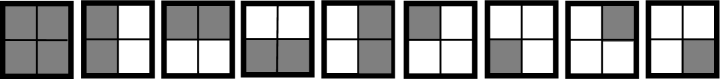
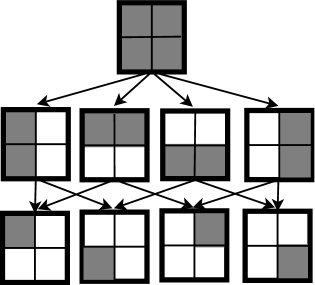
Figure 1: Sparsity patterns of $\mathbf{B}_{\mathbf{h}}^{\mathbf{g}}$ and a DAG constructed with the sparsity patterns. The shaded area shows zero entries. (a) All possible zero patterns of $\mathbf{B}_{\mathbf{h}}^{\mathbf{g}}$ that can be induced by Eq. (5a,5b,5c) when $\mathbf{g}=\{1,2\}$ and $\mathbf{h}=\{1,2\}$. (b) An example of a DAG that contains the zero patterns of $\mathbf{B}_{\mathbf{h}}^{\mathbf{g}}$. The root node contains zero pattern for $\mathbf{B}_{\mathbf{h}}^{\mathbf{g}}=\bm{0}$, and the internal nodes represent the zero patterns for $\bm{\beta}_{\mathbf{h}}^{j}=\bm{0}$ (one column is zero) or $\bm{\beta}_{k}^{\mathbf{g}}=\bm{0}$ (one row is zero). The leaf nodes denote $\beta_{k}^{j}=0$. In the DAG, the zero pattern of children nodes should be a subset of their parent nodes’ zero patterns.

In this section, we propose our method to optimize Eq. (5). We start with a non-zero $\mathbf{B}$ initialized by other methods (e.g. ridge regression), and always reduce the set of non-zero $\beta_{k}^{j}$s using thresholding operations as our procedure proceeds. Our framework is an iterative procedure consisting of two steps. First, we set the groups (or individual) of regression coefficients to zero by checking optimality conditions (called thresholding) as we walk through a predefined directed acyclic graph (DAG). When we walk though the nodes in the DAG, some $\beta_{k}^{j}$s might not achieve zero. Second, we update only these non-zero $\beta_{k}^{j}$s using any available optimization techniques.

Let us first characterize the zero patterns induced by Eq. (5a – 5c). We separately consider a block of $\mathbf{B}$ which consists of one input group $(\mathbf{g}\in\mathcal{G})$ and one output group $(\mathbf{h}\in\mathcal{H})$. Our observation tells us that there are grouping effects (to be zero simultaneously) for each $\mathbf{g}$ and $\mathbf{h}$: $\bm{\beta}_{k}^{\mathbf{g}}=\bm{0}$ and $\bm{\beta}_{\mathbf{h}}^{j}=\bm{0}$. We also have $\mathbf{B}_{{\mathbf{h}}}^{{\mathbf{g}}}=\bm{0}$ when $\bm{\beta}_{k}^{\mathbf{g}}=\bm{0},\;\forall k\in\mathbf{h}$ or $\bm{\beta}_{\mathbf{h}}^{j}=\bm{0},\;\forall j\in\mathbf{g}$. Each covariate can also be zero, i.e, $\beta_{k}^{j}=0$ due to the $\ell_{1}$ penalty in Eq. (5a). Figure 1(a) shows all the possible zero patterns of $\mathbf{B}_{\mathbf{h}}^{\mathbf{g}}$ induced by Eq. (5a – 5c). Given these sparsity patterns, to induce structured sparsity, one might be able to check whether or not these zero patterns satisfy optimality conditions and discard irrelevant covariates accordingly. However, this approach may be inefficient as it needs to examine the large number of zero patterns. Instead, to efficiently check the zero patterns, we will construct a DAG, and exploit the inclusion relationships between the zero patterns. The main idea is that we want to be able to check all zero patterns by traversing the DAG while avoiding unnecessary optimality checks.

In Figure 1(b), we show an example of the DAG for $\mathbf{B}_{\mathbf{h}}^{\mathbf{g}}$ when $\mathbf{g}=\{1,2\}$ and $\mathbf{h}=\{1,2\}$. We denote the set of all possible zero patterns of $\mathbf{B}$ by $\mathcal{Z}=\{Z_{1},\ldots,Z_{|\mathcal{Z}|}\}$. For example, $Z_{1}$ can be a zero pattern for $\mathbf{B}_{\mathbf{h}}^{\mathbf{g}}=\bm{0}$ (the root node in Figure 1(b)). Let us denote $\mathbf{B}(Z_{t})$ by the coefficients of $\mathbf{B}$ corresponding to $Z_{t}$’s zero pattern. Then we define the DAG as follows: A node is represented by $Z\in\mathcal{Z}$, and there exists a directed edge from $Z_{1}\in\mathcal{Z}$ to $Z_{2}\in\mathcal{Z}$ if and only if $Z_{1}\supset Z_{2}$ and $\nexists Z\in\mathcal{Z}:Z_{1}\supset Z\supset Z_{2}$. For example, in Figure 1(b), the zero patterns of the nodes in the second level include the zero patterns of their children. In general, when we have multiple input and output groups, we can generate a DAG for each $\mathbf{B}_{{\mathbf{h}}}^{{\mathbf{g}}}$ separately and then connect all the DAGs to the root node for $\mathbf{B}=\bm{0}$. This graph is originated from Hasse diagram cameron1994combinatorics and it was previously utilized for finding a minimal set of groups for inducing structured sparsity jenatton2009structured .

We can readily observe that our procedure has the following properties:

• Walking through the DAG, we can check all possible zero patterns explicitly without resorting to heuristics or approximations.

• If $\mathbf{B}(Z)=\bm{0},\;Z\in\mathcal{Z}$, we know that all the descendants of $Z$ are also zero due to the inclusion relations of the DAG. Hence, we can “skip” to check the optimality conditions that the descendants of $Z$ are zero.

Considering these properties, we develop our optimization framework for the following reasons. First, we can achieve accurate zero patterns in $\mathbf{B}$ since we check all possible sparsity patterns when walking through the DAG. Second, if $\mathbf{B}$ is sparse, our framework is very efficient since we can skip the optimality checks for many zero patterns in $\mathcal{Z}$. Mostly we will check only nodes located at the high levels of the DAG. Third, our framework is simple to implement. All we need is to check whether each node in the DAG attains zero and update non-zero $\beta_{k}^{j}$s only when necessary.

Specifically, our hierarchical group-thresholding employs the following procedure:

1. Initialize a non-zero $\mathbf{B}$ using any available methods (e.g. ridge regression).

2. Construct a DAG that contains all zero patterns of $\mathbf{B}$ that can be induced by the penalty in Eq. (5a, 5b, 5c).

3. Use depth-first-search (DFS) to traverse the DAG, and check the optimality conditions to see if the zero patterns at each node $Z$ achieve zero. If $\mathbf{B}(Z)=0$ or $Z$ satisfies the optimality condition to be zero, set $\mathbf{B}(Z)=0$, skip the descendants of $Z$, and visit the next node according to the DFS order.

4. For those of $\beta_{k}^{j}$’s which did not achieve zero in the previous step, update the coefficients of the non-zero $\beta_{k}^{j}$’s using any available optimization algorithms.

5. Iterate step 3 and 4 until Eq. (5) converges.

Bellow we briefly present the derivations of the three ingredients of our optimization framework that include 1) the construction of a DAG, 2) the optimality condition of each $Z\in\mathcal{Z}$ in the DAG and 3) the rule for updating non-zero regression coefficients. Our optimization method is summarized in Algorithm 1.

Algorithm 1 Hierarchical group-thresholding method for Eq. (5)

 $\mathbf{B}\leftarrow\mbox{coefficients estimated by ridge regression}$

 $\mathcal{G}\leftarrow\mbox{groups of inputs}$

 $\mathcal{H}\leftarrow\mbox{groups of outputs}$

 $D(\mathcal{Z},\mathcal{E})\leftarrow\mbox{DAG including all zero patterns}$

 $\{Z_{(1)},Z_{(2)},\ldots,Z_{(|\mathcal{Z}|)}\}\leftarrow\mbox{DFS order of $\mathcal{Z}$ in $D$}$

 repeat

    $t\leftarrow 1$

    while $t\leq|\mathcal{Z}|$ do

       if $Z_{(t)}$ contains $\mathbf{B}_{\mathbf{h}}^{\mathbf{g}}=\bm{0}$ then

          c $\leftarrow$ Eq. (10)

       else if $Z_{(t)}$ contains $\bm{\beta}_{k}^{\mathbf{g}}=\bm{0}$ then

          c $\leftarrow$ Eq. (11)

       else if $Z_{(t)}$ contains $\bm{\beta}_{\mathbf{h}}^{j}=\bm{0}$ then

          c $\leftarrow$ Eq. (12)

       else if $Z_{(t)}$ contains $\beta_{k}^{j}=0$ then

          c $\leftarrow$ Eq. (13)

       end if

       if c holds (condition for $\mathbf{B}(Z_{(t)})=\bm{0}$) or $\mathbf{B}(Z_{(t)})=\bm{0}$ then

          $\mathbf{B}(Z_{(t)})=\bm{0}$ (Set zero to $Z_{(t)}$’s zero pattern)

          $t\leftarrow$ DFS order of $t^{\prime}$ such that $Z_{(t^{\prime})}$ is not a descendant of $Z_{(t)}$, $t^{\prime}>t$ and $\nexists t{{}^{\prime\prime}}:t^{\prime}>t{{}^{\prime\prime}}>t$ (Skip the descendants of $Z_{(t)}$)

       else if c $=$ Eq. (13) then

          Update $\beta_{k}^{j}$ using Eq. (14) (Updating non-zero regression coefficients)

          $t\leftarrow t+1$

       else

          $t\leftarrow t+1$

       end if

    end while

 until convergence

Construction of the DAG

To generate the DAG, first we define the set of nodes $\mathcal{Z}$. For each block of $\mathbf{B}_{\mathbf{h}}^{\mathbf{g}}$, we are interested in the four types of zero patterns as follows:

1. $\mathbf{B}_{{\mathbf{h}}}^{{\mathbf{g}}}$ is zero: $\mathbf{B}_{{\mathbf{h}}}^{{\mathbf{g}}}=\bm{0}$.

2. One row in $\mathbf{B}_{{\mathbf{h}}}^{{\mathbf{g}}}$ is zero: $\bm{\beta}_{k}^{{\mathbf{g}}}=\bm{0}$, $k\in{\mathbf{h}}$.

3. One column in $\mathbf{B}_{{\mathbf{h}}}^{{\mathbf{g}}}$ is zero: $\bm{\beta}_{{\mathbf{h}}}^{j}=\bm{0}$, $j\in{\mathbf{g}}$.

4. One regression coefficient in $\mathbf{B}_{{\mathbf{h}}}^{{\mathbf{g}}}$ is zero: $\beta_{k}^{j}=0$, $k\in{\mathbf{h}}$ and $j\in{\mathbf{g}}$.

These zero patterns of $\mathbf{B}$ are shown in Figure 1(b) when $|\mathbf{g}|=|\mathbf{h}|=2$. For example, Case 2 and 3 correspond to the nodes at the second level of the DAG. For all $\mathbf{g}\in\mathcal{G}$ and $\mathbf{h}\in\mathcal{H}$, we can define nodes $Z\in\mathcal{Z}$ using the above zero patterns. Then we need to determine the edges of the DAG by investigating the relations of the nodes. We can also easily see that there exists the relationship among the zero patterns: $\mbox{Case }1\supset\mbox{Case }2,\mbox{Case }3\supset\mbox{Case }4$. Given the zero patterns and their relations, we create a directed edge $Z_{1}\rightarrow Z_{2}$ if and only if $Z_{1}\supset Z_{2}$ and $\nexists Z\in\mathcal{Z}:Z_{1}\supset Z\supset Z_{2}$. In Figure 1(b) we show an example of the DAG. Finally, we make a dummy root node and generate an edge from the dummy node to the root of all DAGs for $\mathbf{B}_{{\mathbf{h}}}^{{\mathbf{g}}}=\bm{0}$.

Optimality conditions for structured sparsity patterns

Given a block of $\mathbf{B}_{\mathbf{h}}^{\mathbf{g}}$, here we show optimality conditions for the four sparsity patterns: (1) $\mathbf{B}_{\mathbf{h}}^{\mathbf{g}}=\bm{0}$, (2) $\bm{\beta}_{k}^{\mathbf{g}}=\bm{0}$, (3) $\bm{\beta}_{\mathbf{h}}^{j}=\bm{0}$, and (4) $\beta_{k}^{j}=0$, ($j\in\mathbf{g},k\in\mathbf{h},\mathbf{g}\in\mathcal{G},\mathbf{h}\in\mathcal{H}$). In Figure 1(b), the root node corresponds to the first case, the nodes at the second level correspond to the second and third case, and the leaf nodes correspond to the fourth case. Our derivation of the following optimality conditions use the fact that all zero coefficients are fixed, as it makes it simple to deal with overlapping groups. We denote the column and row indices of zero entries by $\bm{\eta}=\{j:\beta_{k}^{j}=0,\;\forall j\in\mathbf{g},\;\forall k\in\mathbf{h}\}$ and $\bm{\gamma}=\{k:\beta_{k}^{j}=0,\;\forall j\in\mathbf{g},\;\forall k\in\mathbf{h}\}$.

First, the optimality condition for the first case is as follows: $\mathbf{B}_{\mathbf{h}}^{\mathbf{g}}=\bm{0}$ if

$$\sum_{k\in\mathbf{h}-\bm{\gamma}}\sum_{j\in\mathbf{g}-\bm{\eta}}\left\{{\mathbf{r}}_{k}^{j}(\mathbf{x}_{j})^{T}-\lambda_{1}s_{k}^{j}\right\}^{2}\leq\left(\lambda_{2}\sqrt{|\mathbf{h}|}+\lambda_{3}\sqrt{|\mathbf{g}|}\right)^{2},$$ (10)

where

$$s_{k}^{j}=\left\{\begin{array}[]{l l}\frac{{\mathbf{r}}_{k}^{j}(\mathbf{x}_{j})^{T}}{\lambda_{1}}&\mbox{if $\left|\frac{{\mathbf{r}}_{k}^{j}(\mathbf{x}_{j})^{T}}{\lambda_{1}}\right|\leq 1$}\\ sign\left(\frac{{\mathbf{r}}_{k}^{j}(\mathbf{x}_{j})^{T}}{\lambda_{1}}\right)&\mbox{if $\left|\frac{{\mathbf{r}}_{k}^{j}(\mathbf{x}_{j})^{T}}{\lambda_{1}}\right|>1$}.\\ \end{array}\right.$$

It is derived using KKT condition in Eq. (6) and Cauchy-Schwarz inequality.

The second case of structured sparsity, i.e, $\bm{\beta}_{k}^{\mathbf{g}}=\bm{0}$ is achieved if

$$\sum_{j\in{\mathbf{g}-\bm{\eta}}}\left\{{\mathbf{r}}_{k}^{j}(\mathbf{x}_{j})^{T}-\lambda_{1}s_{k}^{j}\right\}^{2}\leq\lambda_{2}^{2},$$ (11)

and the optimality condition for the third case, i.e, $\bm{\beta}_{\mathbf{h}}^{j}=\bm{0}$ is

$$\sum_{k\in\mathbf{h}-\bm{\gamma}}\left\{{\mathbf{r}}_{k}^{j}(\mathbf{x}_{j})^{T}-\lambda_{1}s_{k}^{j}\right\}^{2}\leq\lambda_{3}^{2}.$$ (12)

These conditions can be established using KKT condition in Eq. (6) fixing all the zero coefficients. Finally, assuming that $\bm{\beta}_{\mathbf{h}}^{j}\neq\bm{0}$ and $\bm{\beta}_{k}^{\mathbf{g}}\neq\bm{0}$, the fourth case has the optimality condition of

$$|{\mathbf{r}}_{k}^{j}(\mathbf{x}_{j})^{T}|\leq\lambda_{1}.$$ (13)

Update rule for nonzero coefficients

If all the above optimality conditions do not hold, we know that $\beta_{k}^{j}\neq 0$. In this case, the gradient of Eq. (5) with respect to $\beta_{k}^{j}$ exists, and we can update $\beta_{k}^{j}$ using any coordinate descent procedures. With a little bit of algebra, we derive the following update rule: $\beta_{k}^{j}=\hat{\beta}_{k,-}^{j}+\hat{\beta}_{k,+}^{j}$ where

$$\hat{\beta}_{k,-}^{j} =\min\left[0,\left(1+\sum_{j\in\mathbf{g}}\frac{\lambda_{2}}{\left\|\bm{\beta}_{k}^{\mathbf{g}}\right\|_{2}}+\sum_{k\in\mathbf{h}}\frac{\lambda_{3}}{\left\|\bm{\beta}_{\mathbf{h}}^{j}\right\|_{2}}\right)^{-1}\left\{\mathbf{r}_{k}(\mathbf{x}_{j})^{T}+\lambda_{1}\right\}\right],$$ (14)

$$\hat{\beta}_{k,+}^{j} =\max\left[0,\left(1+\sum_{j\in\mathbf{g}}\frac{\lambda_{2}}{\left\|\bm{\beta}_{k}^{\mathbf{g}}\right\|_{2}}+\sum_{k\in\mathbf{h}}\frac{\lambda_{3}}{\left\|\bm{\beta}_{\mathbf{h}}^{j}\right\|_{2}}\right)^{-1}\left\{\mathbf{r}_{k}(\mathbf{x}_{j})^{T}-\lambda_{1}\right\}\right].$$

We close this section by summarizing the desirable properties of our optimization method. First, when $\mathbf{B}$ is sparse, our optimization procedure is very fast. We take advantage of not only the hierarchical structure of the DAG, but also the simple forms of the optimality conditions with residuals. If we keep track of the residuals, we can efficiently check the optimality conditions for each sparsity pattern. Second, our thresholding operations check all possible sparsity patterns, resulting in appropriate structured sparsity in $\mathbf{B}$. It is important for eQTL mapping since the coefficients for irrelevant SNPs can be set to exactly zero. Third, our optimization method can deal with overlaps between/within the coefficients for input groups ($\bm{\beta}_{k}^{\mathbf{g}}$’s) and output groups ($\bm{\beta}_{\mathbf{h}}^{j}$’s). Since input or output groups may overlap, and they must be considered simultaneously, this property of our method is essential. Finally, unlike some previous methods yuan2006model ; tibshirani1996regression , we make no use of the assumption that the design matrix $\mathbf{X}$ is orthonormal ($\mathbf{X}^{T}\mathbf{X}=\mathbf{I}$). This dropping of the assumption is desirable for eQTL mapping in particular as covariates (SNPs) are highly correlated due to linkage disequilibrium. If one uses orthonormalization as a preprocessing step to make $\mathbf{X}$ orthonormal, there is no guarantee that the same solution for the original problem is attained friedman2010note .

5 Dealing with structures inducing higher-order effects

So far, we have been dealing with input and output structures in the context of multi-variate and multi-task linear regression where the influences from the covariates on the responses are additive. When higher interactions take place among covariates, which is known as epistasis and is prevalent in genetic associations carlson2004mapping , a common approach to model such effects is polynomial regression montgomery2001introduction , where higher-order terms of the covariates are included as additional regressors. However, in high-dimensional problems such as the one studied in this paper, this strategy is infeasible even for 2nd-order polynomial regression because, given say, even a standard genome dataset with $\sim 10^{5}$ SNPs, one is left with $\sim 10^{10}$ regressors which is both computationally and statistically unmanageable. In this section, we briefly show how to circumvent this difficulty using structured regularization based on prior information of covariate interactions. This strategy is essentially a straightforward generalization of the ideas in Section 3 to a polynomial regression setting using a special type of structure encoded by a graph. Therefore all the algorithmic solutions developed in Section 4 for the general optimization problem in Section 3 still apply here.

Following common practice in GWA literature, here we consider only 2nd-order interactions between SNP pairs. Instead of including all SNP pairs as regressors, we employ a synthetic genetic interaction network costanzo2010genetic to define a relatively small candidate set ${\bf U}$ of interacting SNP pairs. A synthetic genetic interaction network is derived from biological evidences of pairwise functional interactions between genes, such as double knockout experiments tong2004global ; koh2009drygin ; costanzo2010genetic ; boone2007exploring . It contains information about the pairs of genes whose mutations affect the phenotype only when the mutations are present on both genes, and this represents a set of ground-truth interaction effects. Given such a network, we consider only those pairs of SNPs that are physically located in the genome near the genes that interact in the network within a certain distance. A 2nd-order regressor set ${\bf U}$ generated by this scheme is not only much smaller than an exhaustive pair-set, but also biologically more plausible. Note that it is possible to include other sets of SNP pairs from other resources in our candidate set. For example, in our experiments, we also added SNP pairs that passed two-locus epistasis test with p-value $<10^{-5}$ into the set ${\bf U}$.

After finding the candidate SNP pairs, we generate the group of SNPs or interacting SNP pairs in two steps. In the first step, we find highly interconnected subgraphs (or clusters) from the genetic interaction network using any graph clustering algorithms. In our experiments, we used MCODE algorithm bader2003automated for clustering the network. In the second step, we group all the SNPs or SNP pairs that are linked to the genes in a cluster. We linked the genes and SNPs based on physical locations in the genome. For example, if a SNP is located nearby a gene within a certain distance (e.g. $<$500bp), they are linked together. Finally, we define individual SNPs in the $m$th group as ${\mathbf{g}}_{m}\in\mathcal{G}$ and SNP pairs in the $m$th group as ${\mathbf{l}}_{m}\in\mathcal{L}$. We then look for associations between inputs/input-pairs and outputs via Eq. (15):

$$\min\frac{1}{2}\sum_{k=1}^{K}\sum_{i=1}^{N} \left(y_{k}^{i}-\sum_{j=1}^{J}{\beta_{k}^{j}x_{j}^{i}}-\sum_{(r,s)\in{\bf U}}{\beta_{k}^{rs}x_{r}^{i}x_{s}^{i}}\right)^{2}$$ (15a)

$$+\lambda_{1}\sum_{k=1}^{K}\sum_{j=1}^{J}{|\beta_{k}^{j}|}$$ (15b)

$$+\lambda_{2}\sum_{k=1}^{K}\left(\sum_{m=1}^{|\mathcal{G}|}{\sqrt{\sum_{j\in{\mathbf{g}}_{m}}({\beta_{k}^{j}})^{2}}}+\sum_{m=1}^{|\mathcal{L}|}{\sqrt{\sum_{(r,s)\in{\mathbf{l}}_{m}}{(\beta_{k}^{rs}})^{2}}}\right)$$ (15c)

$$+\lambda_{3}\left(\sum_{j=1}^{J}\sum_{m=1}^{|\mathcal{H}|}\sqrt{\sum_{k\in{\mathbf{h}}_{m}}{({\beta_{k}^{j}})^{2}}}+\sum_{(r,s)\in{\bf U}}\sum_{m=1}^{|\mathcal{H}|}\sqrt{\sum_{k\in{\mathbf{h}}_{m}}{({\beta_{k}^{rs}})^{2}}}\right)$$ (15d)

$$+\lambda_{4}\sum_{k=1}^{K}\sum_{\begin{subarray}{l}(r,s)\in{\bf U}\end{subarray}}{|\beta_{k}^{rs}|}.$$ (15e)

where $\mathcal{G}$ is the set of input groups for marginal terms and $\mathcal{L}$ is the set of input groups for pairwise interaction terms. Here, we use two tuning parameters for $L_{1}$ penalty depending on whether a covariate is modeling an individual effect ($\lambda_{1}$) or interaction effect ($\lambda_{4}$) because they might need different levels of sparsity. Note that this problem is identical to Eq. (5) if we treat interaction terms $x_{r}^{i}x_{s}^{i}$ as additional covariates, and hence our optimization method presented in Section 4 is applicable to Eq. (15). However, Eq. (15) will be more computationally expensive than Eq. (5) since Eq. (15) has a larger number of covariates in $\mathbf{B}$ including both marginal and interaction terms and additional tuning parameter $\lambda_{4}$.

6 Simulation Study

In this section we validate our proposed method using simulated genome/phenome datasets, and examine the effects of simultaneous use of input and output structures on the detection of true non-zero regression coefficients. We also evaluate the speed and the performance of our optimization method for support recovery in comparison to two other alternative methods. For the comparison of optimization methods, we selected smoothing proximal gradient method chen2010efficient and the union of supports jacob2009group since both methods are in principle able to use input/output structures and handle overlapping groups.

The simulated datasets with $J=120,K=80$, and $N=100$ are generated as follows. For generating $\mathbf{X}$, we first selected 60 input covariates from a uniform distribution over $\{0,1\}$ which indicates major or minor genotype. We then simulated 60 pairwise interaction terms $(x_{j}^{i}\times x_{j^{\prime}}^{i})$ by randomly selecting input-pairs from the 60 covariates mentioned above. Pooling the 60 marginal terms and 60 pairwise interaction terms resulted in a input space of 120 dimensions. We also defined input and output groups as follows (for the sake of illustration and comprehension convenience, here our input and output groups correspond to variables to be jointly selected rather than jointly shrunk, the shrinkage penalty in our regression loss can be defined on the complements of these groups):

$$\hbox to0.0pt{$\overbrace{\phantom{5,\ldots,9,10}}^{\mathbf{g}_{1}}$\hss}5,\ldots,\underbrace{9,10,\ldots,15}_{\mathbf{g}_{2}},\ldots,\hbox to0.0pt{$\overbrace{\phantom{25,\ldots,29,30,31,32}}^{\mathbf{g}_{3}}$\hss}25,\ldots,\underbrace{29,30,31,32,\ldots,37}_{\mathbf{g}_{4}},\ldots,\hbox to0.0pt{$\overbrace{\phantom{50,\ldots,54,55,56,57}}^{\mathbf{g}_{5}}$\hss}50,\ldots,\underbrace{54,55,56,57,\ldots,60}_{\mathbf{g}_{6}},\ldots,\hbox to0.0pt{$\overbrace{\phantom{75,\ldots,80,\ldots,87}}^{\mathbf{g}_{7}}$\hss}75,\ldots,\underbrace{80,\ldots,87,\ldots,94}_{\mathbf{g}_{8}},\ldots,\hbox to0.0pt{$\overbrace{\phantom{104,\ldots,109,110,111}}^{\mathbf{g}_{9}}$\hss}104,\ldots,\underbrace{109,110,111,\ldots,116}_{\mathbf{g}_{10}}$$

$$\hbox to0.0pt{$\overbrace{\phantom{1,\ldots,4,5}}^{\mathbf{h}_{1}}$\hss}1,\ldots,\underbrace{4,5,\ldots,10}_{\mathbf{h}_{2}},\ldots,\hbox to0.0pt{$\overbrace{\phantom{12,\ldots,17,18,19,20}}^{\mathbf{h}_{3}}$\hss}12,\ldots,\underbrace{17,18,19,20,\ldots,25}_{\mathbf{h}_{4}},\ldots,\hbox to0.0pt{$\overbrace{\phantom{46,\ldots,56,\ldots,63}}^{\mathbf{h}_{5}}$\hss}46,\ldots,\underbrace{56,\ldots,63,\ldots,70}_{\mathbf{h}_{6}},\ldots,\underbrace{75,\ldots,80}_{\mathbf{h}_{7}},$$

where the numbers within a bracket represent the indices of inputs or outputs for an input group $\mathbf{g}_{t},\;t=1,\ldots,10$, or an output group $\mathbf{h}_{o},\;o=1,\ldots,7$. The inputs and outputs which did not belong to any groups were in a group by itself. We then simulated $\mathbf{B}$, i.e, the ground truth that we want to discover. We selected non-zero coefficients so that $\mathbf{B}$ includes various cases, e.g., overlap between input and output groups, overlap within input groups, and overlap within output groups. Figure 2(a) shows the simulated $\mathbf{B}\in\mathbb{R}^{80\times 120}$ where non-zero coefficients are represented by black blocks. Given $\mathbf{X}$ and $\mathbf{B}$, we generated $K=80$ outputs by $\mathbf{Y}=\mathbf{B}\mathbf{X}+\mathbf{E},$ $\mathbf{E}\sim\mathcal{N}(\bm{0},\mathbf{I})$. We generated 20 datasets and optimized Eq. (5) using the three methods. We report the average performance using precision recall curves.

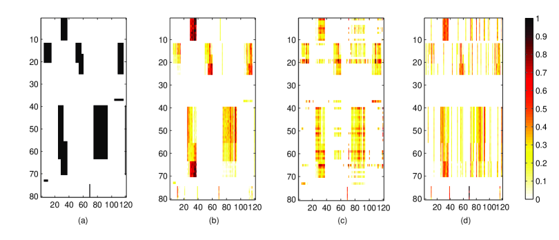
Figure 2: An example of simulation results with $|\beta_{k}^{j}|=2,N=100,J=120$, and $K=80$. (a) True regression coefficient matrix. Estimated $\mathbf{B}$ by SIOL (b) with both input and output structures (c) with only input structure, and (d) with only output structure. In (b-d), we show the normalized values of $|\mathbf{B}|$.

6.1 Evaluation of the Effects of Using Input and Output Structures

We first investigate the effects of using both input and output structures on the performance of our model. Here we applied our optimization method (HiGT) to the following three models with different use of structural information:

1. Use of both input and output structures (Eq. (5a) + Eq. (5b) + Eq. (5c))

2. Use of input structures (Eq. (5a) + Eq. (5b))

3. Use of output structures (Eq. (5a) + Eq. (5c))

We then observed how the use of input/output structures affect the recovery of the true non-zero coefficients and the prediction error. In Figure 2, we visualize the examples of estimated $\mathbf{B}$ by the three different models. Figure 2(b) shows that the model with input and output structure successfully recovered true regression coefficients in Figure 2(a). However, as shown in Figure 2(c-d), the models with either input or output structure were less effective to suppress noisy signals, which resulted in many false positives.

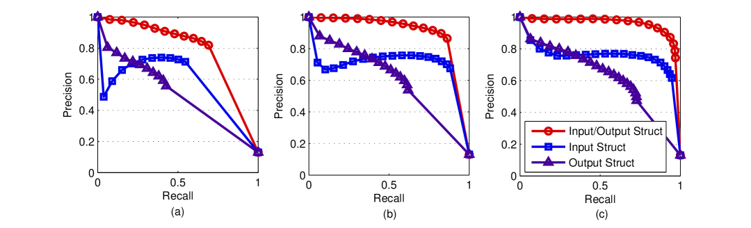
Figure 3: Precision recall curves on the recovery of true non-zero coefficients due to SIOL with both input and output structures (input/output struct), regression with only input structure (input struct), and with only output structure (output struct), under three different signal strengths of true regression coefficients. (a) $\beta_{k}^{j}=0.4$, (b) $\beta_{k}^{j}=1$, and (c) $\beta_{k}^{j}=2$. The simulated data were generated with $N=100,J=120$, and $K=80$.

Figure 3 shows the precision recall curves on the recovery of true non-zero coefficients by changing the threshold $\tau$ for choosing relevant covariates ($|\beta_{k}^{j}|>\tau$), under different signal strengths of 0.4, 1 and 2. For all signal strengths, the model with input/output structures significantly outperformed the other models with either input or output structure. The most interesting result is that when the signal strength was very small such as 0.4, our model still achieved good performance by taking advantage of both structural information.

Figure 4: Comparison of the prediction error of SIOL (input/output struct), with regression under only input structure (input struct), on only output structure (output struct). (a) $\beta_{k}^{j}=0.4$, (b) $\beta_{k}^{j}=1$, (c) $\beta_{k}^{j}=2$.

We also compare the prediction errors on our validation data with 280 ($20\times 14$) samples (each dataset had 14 samples for validation). For computing the prediction error, we first selected non-zero coefficients, and then recomputed the coefficients of those selected covariates using linear regression without shrinkage penalty. Using the unbiased coefficients of the chosen covariates, we measured the prediction error for our validation data. Figure 4 shows the prediction error under different signal strengths ranging from 0.4 to 2. For all signal strengths, we obtained significantly better prediction error using both input and output structures. When the signal strength was large such as 1 or 2, the use of both input and output structures was especially beneficial for reducing the prediction error since it helped the model to find most of the true covariates relevant to the outputs.

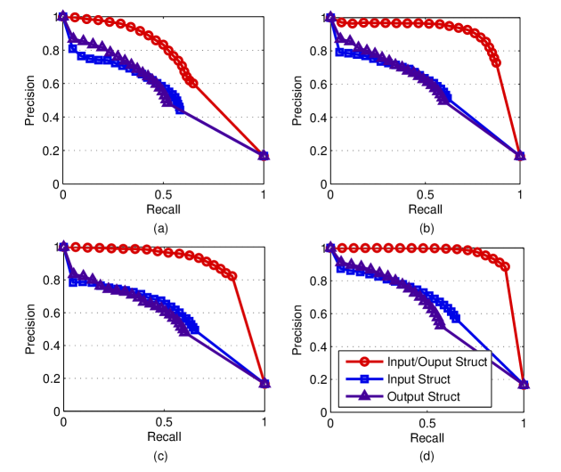
Figure 5: Precision recall curves on the recovery of true non-zero coefficients for SIOL (input/output struct), regression with only input structure, and with only output structure, under two different sizes of input and output groups. (a) $|g|\in\{2,3\}$, (b) $|g|=5,\;\forall g\in\mathcal{G}$, and (c) $|h|=5$, and (d) $|h|=40,\;\forall h\in\mathcal{H}$. We fixed the size of output groups for (a,b) ($|h|=10$), and fixed the size of input groups for (c,d) ($|g|=5$). The simulated data were generated with $\beta_{k}^{j}=0.5$, $N=100$, and $J=120$.

The effects of the size of input and output groups

Figure (5a-5d) demonstrates the results on simulated datasets with different size of input and output groups. For all group sizes, our method significantly improved the performance by effectively taking advantage of both input and output groups.

6.2 Comparison of HiGT to Alternative Optimization Methods

In this section, we compare the accuracy and speed of our optimization method (HiGT) with those of the two alternative methods including smoothing proximal gradient method (SPG) chen2010efficient and union of supports jacob2009group . Both alternatives can handle overlapping groups. Specifically, the smoothing proximal gradient method is developed to efficiently deal with overlapping group lasso penalty and graph-guided fusion penalty using an approximation approach. However, it may be inappropriate for our model since the maximum gap between the approximated penalty and the exact penalty is proportional to the total number of groups $R$, where $R=J|\mathcal{H}|+K|\mathcal{G}|$. Thus, when dealing with high dimensional data (e.g $J\sim 500,000$) such as genome data, the gap will be large, and the approximation method can be severely affected. On the other hand, “union of supports” finds the support of $\mathbf{B}$ from the union support of overlapping groups. To obtain the union of supports, input variables are duplicated to convert the penalty with overlap into the one with disjoint groups, and a standard optimization technique for group lasso yuan2006model can be applied. One of disadvantages of union of supports is that the number of duplicated input variables increases dramatically when we have a large number of overlapping groups. In our experiment, we considered all possible combinations of overlapping input and output groups, and used a coordinate descent algorithm for sparse group lasso friedman2010note .

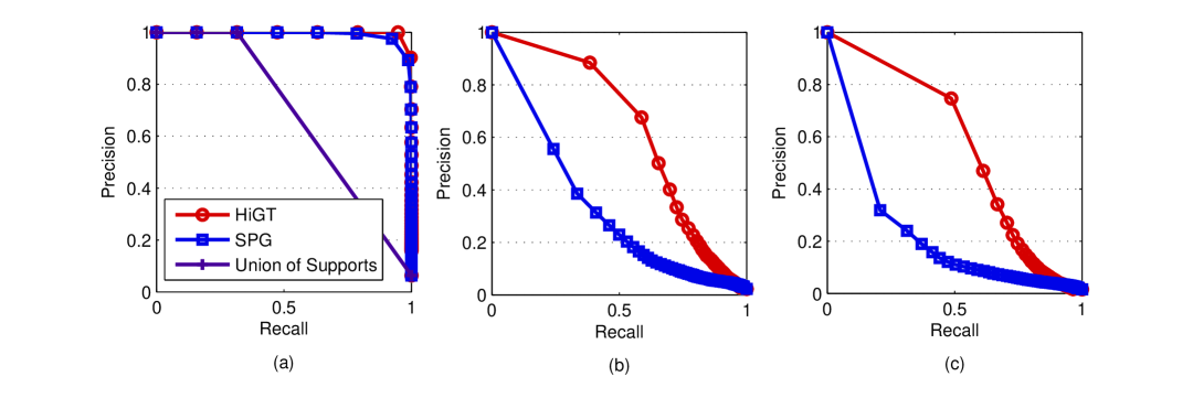
Figure 6: Precision recall curves on the recovery of true non-zero coefficients using the SIOL model via HiGT, smoothing proximal gradient method (SPG), and union of supports for optimization. Three different model sizes determined by the number of input variables were tested (due to high computational cost, results of union-of-support are only available for the smallest problem sizes tested): (a) $J=30$, (b) $J=400$, and (c) $J=600$. The simulated data were generated with $\beta_{k}^{j}=2$, $N=100$, and $K=20$.

Figure 6 shows the precision recall curves on the recovery of true non-zero coefficients under the SIOL model using the three optimization methods. The size of the problem is controlled by increasing number of input variables (from 30 to 600). The simulated data set used here was identical to the data in Section 6.1 except that we used 20 outputs ($\mathbf{y}_{61},\ldots,\mathbf{y}_{80}$) and different number of input variables. One can see that our method outperforms the other alternatives for all configurations. Our method and smoothing proximal gradient method showed similar performance when the input variable is small ($J=30$) but as $J$ increases, our method significantly performed better than SPG. It is consistent with our claim for the maximum gap between the approximated penalty and the exact penalty which is related to the number of groups. Union of supports did not work well even when the number of input variables is small ($J=30$) since the actual number of input variables considered was very large due to the duplicated covariates, which severely degraded the performance.

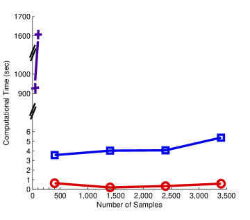
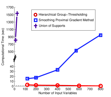
Figure 7: Time complexity of HiGT, SPG, and union of supports. All three methods used both input and output groups. (a) Computational time with different number of samples, (b) computational time with different number of inputs. We used the same tuning parameters for all the methods ($\lambda_{1}=0.01,\lambda_{2}=\lambda_{3}=0.1$). We did not report the times for the small number of samples and inputs for our method and SPG since I/O latency was dominant.

We also compared the speed of our method with the two alternatives of union of supports with all possible combinations of input and output groups and SPG that considered both input and output groups. Figure 7(a,b) show that our method converged faster than the other competitors, and was significantly more scalable than the two alternatives. Union of supports was very slow compared to our method and SPG because of the large number of duplicated input variables. Our experimental results confirms that our optimization technique is not only accurate but also fast, which can be explained by the use of DAG and the simple forms of optimality checks.

7 Analysis of Yeast eQTL Dataset

We apply our method to the budding yeast (Saccharomyces cerevisiae) data brem2005landscape with 1,260 unique SNPs (out of 2,956 SNPs) and the observed gene-expression levels of 5,637 genes. As network prior knowledge, we used genetic interaction network reported in costanzo2010genetic with stringent cutoff to construct the set of candidates of SNP pairs ${\bf U}$. We follow the procedure in section 5 to make ${\bf U}$ with an additional set of significant SNP pairs with p-value $<10^{-5}$ computed from two-locus epistasis test. When determining the set ${\bf U}$, we assumed that a SNP is linked to a gene if the distance between them is less than 500bp. We consider it a reasonable choice for cis-effect as the size of intergene regions for S. cerevisiae is 515bp on average sunnerhagen2006comparative . As a result, we included 982 interaction terms from the interaction network in $\mathbf{X}$ with 1,260 individual SNPs. The number of SNP pairs from two-locus epistasis test varied depending on the trait. For generating input structures, we processed the network data as follows. We started with genetic interaction data which include 74,984 interactions between gene pairs. We then extracted genetic interactions with low p-values ($<$0.001). Given 44,056 significant interactions, using MCODE clustering algorithm, we found 55 gene clusters. Using the gene clusters, we generated the groups of individual SNPs and pairs of SNPs according to the scheme in section 5. For generating output structures, we applied hierarchical clustering to the yeast gene expression data with cutoff 0.8, resulting in 2,233 trait clusters.

Marginal Effects in Yeast eQTL dataset

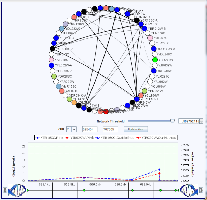
Figure 8: Manhattan plot for association between (YER160C and YJR029W) and SNPs on chromosome 7. The two genes YER160C and YJR029W share the same GO category “transposition”. Our method detected SNPs which affect both two genes in this region. However, single SNP analysis did not find any associated SNPs and lasso found SNPs associated only with YER160C in this region. Graph were generated using the GenAMap software curtisgenamap .

We briefly demonstrate the effects of input/output structures on the detection of eQTLs with marginal effects. In general, the association results for marginal effects by our method, lasso and single SNP analysis (the later two are standard methods in contemporary GWA mapping that use no structural information, and hence included for comparison) showed similar patterns for strong associations. However, we observed differences for SNPs with small or medium sized signals. For example, our results had fewer nonzero regression coefficients compared to lasso. One possible explanation would be that the grouping effects induced by our model with input/output structures might have removed false predictions with small or medium sized effects. To illustrate eQTLs with marginal effects, we show some examples of association SNPs using GenAMap curtisgenamap . Figure 8 demonstrates a Manhattan plot on chromosome 7 for two genes including YER160C and YJR029W. Both genes have the same GO category “transposition”. As both genes share the same GO category, it is likely that they are affected by the same SNPs if there exist any association SNPs for both genes. In our results, we could see that the same SNPs on chromosome 7 are associated with both genes as shown in Figure 8. However, single SNP analysis did not find any significant association SNPs in the region. Lasso detected association SNPs in the region but they were associated with only YER160C rather than both of them (lasso plot is not shown to avoid cluttered figure). This observation is interesting since it supports that our method can effectively detect the SNPs jointly associated with the gene traits by taking advantage of structural information.

Epistatic Effects in Yeast eQTL dataset

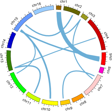
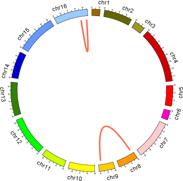
Figure 9: Hotspots with interaction effects identified by (a) our method and (b) two-locus epistasis test. This figure represents the yeast genome in a circular format. In clockwise direction, from the top of the circles, we show 16 chromosomes, which are separated with space and different colors. Lines indicate interaction effects between two connected locations in the genome. Thickness of the lines is proportional to the number of traits affected by the interaction effects. Here we show interaction effects which influence more than 100 gene traits. The hotspots for (a) are represented in Table 1. In (b), two SNP pairs are found including chr16:718892-chr16:890898 (affected genes are enriched with the GO category of ribosome biogenesis with corrected p-value $1.6\times 10^{-36})$, and chr8:56246-chr9:362631 (affected genes are enriched with the GO category of vacuolar protein catabolic process with corrected p-value $1.6\times 10^{-14})$. This figure was generated using Circos software krzywinski2009circos .

Table 1: Hotspots of SNP pairs having epistatic effects in yeast identified by our method.

Hotspot	SNP1	SNP2	Number of	GO category of	Corrected p-value of
label	location	location	affected traits	affected traits	GO category
1	chr1:154328	chr5:350744	455	ribosome biogenesis	$1.2\times 10^{-36}$
2	chr10:380085	chr15:170945	195	ribosome biogenesis	$1.6\times 10^{-12}$
3	chr10:380085	chr15:175594	185	ribosome biogenesis	$4.1\times 10^{-12}$
4	chr5:222998	chr15:108577	170	response to temperature stimulus	$2.9\times 10^{-6}$
5	chr11:388373	chr13:64970	155	regulation of translation	$1.8\times 10^{-32}$
6	chr2:499012	chr15:519764	145	vacuolar protein catabolic process	$1.4\times 10^{-7}$
7	chr1:41483	chr3:64311	130
8	chr7:141949	chr9:277908	125
9	chr3:64311	chr7:312740	115	glycoprotein metabolic process	$1.5\times 10^{-4}$
10	chr12:957108	chr15:170945	110	vacuolar protein catabolic process	$7.8\times 10^{-16}$
11	chr4:864542	chr13:64970	105	ribonucleoprotein complex biogenesis	$3.7\times 10^{-6}$

Now we show the benefits of using the input/output structures for detecting interaction effects among SNPs by comparing the results of our method to those of two-locus epistasis test performed by PLINK purcell2007plink which uses no structural information. Specifically, we compare the hotspots with interaction effects (i.e. SNP pairs that affect a large number of gene traits) which are identified by both methods. Recall that two-locus epistasis test is the most widely used statistical technique for detecting interaction effects in genome-wide association studies, which computes the significance of interactions by comparing between the null model with only two marginal effects and the alternative model with two marginal effects and their interaction effect. In the following analysis, we discarded all SNP pairs if the correlation coefficient between the pairs $>0.5$ to avoid trivial interaction effects.

We first identified the most significant hotspots that affect more than 100 gene traits. To make sure that we include only significant interactions, we considered interaction terms if their absolute value of regression coefficients are $>0.05$. For the results of two-locus epistasis test, we considered all SNP pairs with p-value $<10^{-5}$. Figure 9(a,b) show the hotspots found by our method and two-locus epistasis test. The rings in the figure represent the yeast genome from chromosome 1 (located at the top of each circle) to 16 clockwise, and the lines show interactions between the two genomic locations at both ends. One can see that our method detected 11 hotspots but two-locus epistasis test found only two significant hotspots with interaction effects. This observation shows that our method can find more significant hotspots with improved statistical power due to the use of the input/output structures. In Table 1, we summarized the hotspots found by our method. It turns out that our findings are also biologically interesting (e.g. 9 out of 11 hotspots showed GO enrichment). Notably, hotspot 1 (epistatic interaction between chr1:154328 and chr5:350744) affects 455 genes which are enriched with the GO category of ribosome biogenesis with a significant corrected p-value $<10^{-35}$ (multiple testing correction is performed by false discovery rate maere2005bingo ). This SNP pair was included in our candidates from the genetic interaction network. There is a significant genetic interaction between NUP60 and RAD51 with p-value $3\times 10^{-7}$ costanzo2010genetic , and both genes are located at chr1:152257-153877 and chr5:349975-351178, respectively. As both SNPs are closely located to NUP60 and RAD51 (within 500bp), it is reasonable to hypothesize that two SNPs at chr1:154328 and chr5:350744 affected the two genes, and their genetic interaction in turn acted on a large number of genes related to ribosome biogenesis.

To provide additional biological insights, we further investigated the mechanism of this significant SNP-SNP interaction. From literature survey, RAD51 (RADiation sensitive) is a strand exchange protein involved in DNA repair system sung1994catalysis , and NUP60 (NUclear Pore) is the subunit of unclear pore complex involved in nuclear export system denning2001nucleoporin . Also, it has been reported that yeast cells are excessively sensitive to DNA damaging agents if there exist mutations in NUP60 nagai2008functional . In our results, we also found out that the SNP close to NUP60 did not have significant marginal effects, and the SNP in RAD51 had marginal effects. According to these facts, it would be possible to hypothesize the following. When there is no mutation in RAD51, the point mutation in NUP60 cannot affect other traits since the single mutation is not strong enough and if there exist DNA damaging agents in the environment, DNA repair system would be able to handle them. However, when there exist point mutations in RAD51, DNA damaging agents would severely harm yeast cells with the point mutation in NUP60 since DNA repair system might not work properly due to the mutation in RAD51 (recall that the SNP in RAD51 had marginal effects). As a result, both mutations in NUP60 and RAD51 could make a large impact on many gene traits.

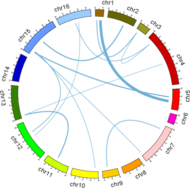
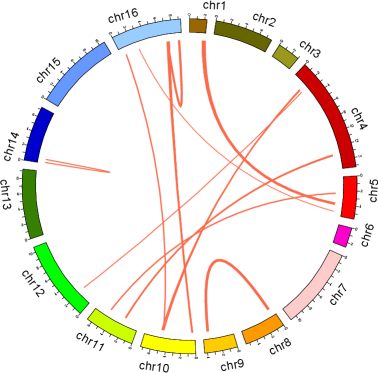
Figure 10: Hotspots with interaction effects identified by (a) our method and (b) two-locus epistasis test by PLINK. Here we show epistatic interactions which influence more than 10 gene traits. This figure was generated using Circos software krzywinski2009circos .

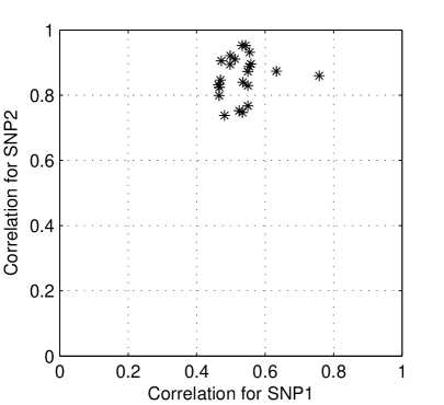
Figure 11: The scatter plot for illustrating the correlation between our epistatic hotspot 1 (chr1:154328-chr5:350744) and significant SNP pairs close to hotspot 1 detected by two-locus epistasis test (p-value $<10^{-6}$ and the distance between the pairs of SNPs and hotspot 1 is within $<50$kb). Each dot represents a SNP pair (SNP1, SNP2) found by two-locus epistasis test, and x-axis represents the correlation between SNP1 and chr1:154328 and y-axis represents the correlation between SNP2 and chr5:350744. Each dot was perturbed by a small amount of random noise to avoid overlapping of the dots.

Furthermore, we looked at the hotspots which affect $>10$ gene traits. Figure 10(a,b) show epistatic interactions identified by our method and two-locus epistasis test, respectively. In this figure, we show significant interactions with regression coefficient cutoff $>0.1$ for our method, and p-value cutoff $<10^{-6}$ for two-locus epistasis test. These cutoffs are arbitrarily chosen to make the number of hotspots found by both methods similar. Surprisingly, two methods showed very different hotspots with epistatic interactions. Figure 10(a) was very similar to Figure 9(a) but in Figure 10(b), several hotspots emerged which were absent in Figure 9(b). We will analyze these hotspots in two ways. First we will look at the hotspots with epistatic effects which appeared in both Figure 10(a) and (b). Then we will investigate the differences between the two results. First, we observed that both methods found significant epistatic effects between chromosome 1 and 5. Recall that in our previous analysis of the hotspots, this interaction was discussed (see hotspot 1 in Table 1). Among all significant SNP pairs found by two-locus epistasis test, there was no identical SNP pair to hotspot 1 but there were 30 SNP pairs close to it (within $<50$kb). Also, it turns out that these 30 SNP pairs had very strong correlation with hotspot 1. In Figure 11, we show scatter plot to illustrate the strong correlations between hotspot 1 and these 30 SNP pairs. More interestingly, the total number of affected traits by these 30 SNP pairs was 416, and it is very similar to 455 that is the number of affected genes by hotspot 1. According to these facts and our previous analysis for the mechanism of hotspot 1, it seems that hotspot 1 is truly significant, and two-locus epistasis test found significant SNP pairs that are close to the true location but failed to locate the exact location of hotspot 1. It supports that our algorithm could find such a significant hotspot affecting $>$ 400 genes by detecting exact SNP pairs. However, two-locus epistasis test was unable to locate many hotspots affecting a large number of traits due to insufficient statistical power. Second, we investigated the differences between the two results in Figure 10(a,b). As we cannot report all the results in the paper, we focused on a SNP pair (chr10:87113-chr15:141621) in Figure 10(a), and another SNP pair (chr8:63314-chr9:362631) in Figure 10(b). Figure 12(a,b) show the average gene expression levels for each SNP pair. In this figure, x-axis represents the genotype $\in\{0,1\}$ which is the multiplication of two SNPs (SNP1 $\times$ SNP2, where SNP1, SNP2 $\in\{0,1\}$), and y-axis represents the average gene expression levels of individuals with given genotype. Each line in Figure 12(a,b) shows how the average gene expression level varies as the genotype changes from 0 to 1 for each trait affected by the SNP pairs with error bars of one standard deviation. Interestingly, in Figure 12(a), we could see that there is a consistent pattern, where for most gene traits, the expression levels decreased as the genotype changed from 0 to 1. However, as shown in Figure 12(b), for the SNP pair found by two-locus epistasis test, we could not find such a coherent pattern. It demonstrates the differences between our method and two-locus epistasis test. As our model borrows information across input and output group structures, we could find consistent gene expression patterns for the SNP pair. On the other hand, two-locus pairwise test analyzed each SNP pair separately, and each trait affected by the SNP pair showed different gene expression patterns with different standard deviations. Thus, it seems that our method can provide interesting biological insights in terms of gene expression patterns in addition to the statistical significance.

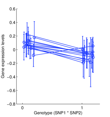
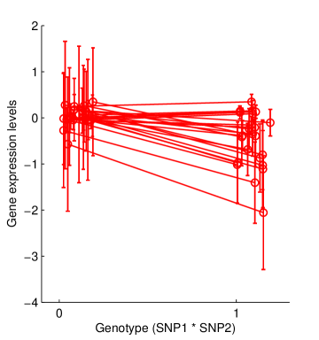
Figure 12: Variations of gene expression levels w.r.t. to the genotypes of (a) a SNP pair (chr10:87113-chr15:141621) found by our method, and (b) a different SNP pair (chr8:63314-chr9:362631) found by two-locus epistasis test. Here, x-axis represents genotype doses and y-axis shows the average expression levels of the multiple genes (denoted by multiple vertical lines) affected by the corresponding SNP pairs. A small noise was added to the genotypes as offsets to avoid overlapping of the error bars.

8 Discussions

In this paper, we presented jointly structured input-output lasso to simultaneously take advantage of both input and output structures. We also presented an efficient optimization technique for solving our multi-task regression model with structured sparsity. Our experiments confirmed that our model is able to significantly improve the accuracy for detecting true non-zero coefficients using both input and output structures. Furthermore, we demonstrated that our optimization method is faster and more accurate than the other competitors. In our analysis of yeast eQTL datasets, we identified important pairs of eQTL hotspots that potentially interact with each other.

Prior knowledge about input and output structures

In practice, it is important to generate reliable input and output groups to maximize the benefits of the structural information. In our experiments, we showed that yeast genetic interaction networks can be used as prior knowledge to define input and output structures. However, such reliable prior knowledge cannot be easily attained when we deal with human eQTL datasets. Instead, we have a variety of resources for human genomes including protein-protein interaction networks and pathway database. Generating reliable input and output structures exploiting multiple resources would be essential for the successful discovery of human eQTLs.

Comparison between HiGT and other optimization algorithms

Recently, an active set algorithm jenatton2009structured has been proposed developed for variable selection with structured sparsity, which can potentially be used for estimating the SIOL model. We observe two key differences between our method and the active set algorithm jenatton2009structured . First, the active set algorithm incrementally increases active sets by searching available non-zero patterns, hence one can see that it is a “bottom-up” approach. On the other hand, our method adopts “top-down” approach where irrelevant covariates are discarded as we walk through the DAG. Second, our algorithm guarantees to search all zero patterns while the active set algorithm needs a heuristic to select candidate non-zero patterns. When $\mathbf{B}$ is sparse, our algorithm is still very fast by taking advantage of the structures of DAG. However, when $\mathbf{B}$ is not sparse, our algorithm needs to search a large number of zero patterns and update many non-zero coefficients but the active set algorithm still does not need to update many non-zero coefficients. Hence, in such a non-sparse case, the active set algorithm may have an advantage over our optimization method. Other alternative optimization methods for SIOL include MM (majorize/minimize) algorithm lange2004springer and generalized stage-wise lasso zhao2007stagewise . However, these methods did not work well for SIOL as the approximated penalty by MM algorithm and the greedy procedure of generalized stage-wise lasso were incapable of efficiently inducing complex sparsity patterns.

Future work

One promising research direction would be to systematically estimate the significance of the covariates that we found. For example, computing p-values of our results would be helpful to control the false discovery rate. To handle both sparse and non-sparse $\mathbf{B}$, it would be also interesting to develop an optimization method for our model that can take advantage of both “bottom-up” and “top-down” strategies. For example, we can select variables using “bottom-up” approach and discard irrelevant variables using ”top-down” approach alternatively in a single framework. Finally, we are interested in applying our method to human disease datasets. In that case, the extension of our work to handle case-control studies and finding reliable structural information will be necessary.

References

- [1] J.L. Badano, C.C. Leitch, S.J. Ansley, H. May-Simera, S. Lawson, R.A. Lewis, P.L. Beales, H.C. Dietz, S. Fisher, and N. Katsanis. Dissection of epistasis in oligogenic bardet–biedl syndrome. Nature, 439(7074):326–330, 2005.
- [2] G. Bader and C. Hogue. An automated method for finding molecular complexes in large protein interaction networks. BMC bioinformatics, 4(1):2, 2003.
- [3] C. Boone, H. Bussey, and B.J. Andrews. Exploring genetic interactions and networks with yeast. Nature Reviews Genetics, 8(6):437–449, 2007.
- [4] R.B. Brem and L. Kruglyak. The landscape of genetic complexity across 5,700 gene expression traits in yeast. PNAS, 102(5):1572, 2005.
- [5] A.A. Brown, S. Richardson, and J. Whittaker. Application of the lasso to expression quantitative trait loci mapping. Statistical Applications in Genetics and Molecular Biology, 10(1):15, 2011.
- [6] P.J. Cameron. Combinatorics: topics, techniques, algorithms. Cambridge Univ Pr, 1994.
- [7] C.S. Carlson, M.A. Eberle, L. Kruglyak, and D.A. Nickerson. Mapping complex disease loci in whole-genome association studies. Nature, 429(6990):446–452, 2004.
- [8] X. Chen, Q. Lin, S. Kim, and E.P. Xing. An efficient proximal-gradient method for single and multi-task regression with structured sparsity. Annals of Applied Statistics, 2010.
- [9] J.H. Cho, D.L. Nicolae, L.H. Gold, C.T. Fields, M.C. LaBuda, P.M. Rohal, M.R. Pickles, L. Qin, Y. Fu, J.S. Mann, et al. Identification of novel susceptibility loci for inflammatory bowel disease on chromosomes 1p, 3q, and 4q: evidence for epistasis between 1p and ibd1. Proceedings of the National Academy of Sciences, 95(13):7502, 1998.
- [10] M. Costanzo et al. The genetic landscape of a cell. Science, 327(5964):425, 2010.
- [11] R.E. Curtis, P. Kinnaird, and E.P. Xing. Genamap: Visualization strategies for structured association mapping.
- [12] D. Denning, B. Mykytka, N.P.C. Allen, L. Huang, AL Burlingame, M. Rexach, et al. The nucleoporin nup60p functions as a gsp1p–gtp-sensitive tether for nup2p at the nuclear pore complex. The Journal of cell biology, 154(5):937–950, 2001.
- [13] B. Devlin, K. Roeder, and L. Wasserman. Analysis of multilocus models of association. Genetic Epidemiology, 25(1):36–47, 2003.
- [14] A.L. Ducrest, L. Keller, and A. Roulin. Pleiotropy in the melanocortin system, coloration and behavioural syndromes. Trends in ecology & evolution, 23(9):502–510, 2008.
- [15] J. Friedman, T. Hastie, H. Hofling, and R. Tibshirani. Pathwise coordinate optimization. Annals of Applied Statistics, 1(2):302–332, 2007.
- [16] J. Friedman, T. Hastie, and R. Tibshirani. A note on the group Lasso and a sparse group Lasso. arXiv:1001.0736v1 [math.ST], 2010.
- [17] Y. Han, F. Wu, J. Jia, Y. Zhuang, and B. Yu. Multi-task sparse discriminant analysis (mtsda) with overlapping categories. In Proceedings of the Twenty-Fourth AAAI Conference on Artificial Intelligence (AAAI-10), pages 469–474, 2010.
- [18] A.E. Hoerl and R.W. Kennard. Ridge regression: Biased estimation for nonorthogonal problems. Technometrics, pages 55–67, 1970.
- [19] L. Jacob, G. Obozinski, and J.P. Vert. Group lasso with overlap and graph lasso. In Proceedings of the 26th Annual International Conference on Machine Learning, pages 433–440. ACM, 2009.
- [20] R. Jenatton, J.Y. Audibert, and F. Bach. Structured variable selection with sparsity-inducing norms. Arxiv preprint arXiv:0904.3523, 2009.
- [21] CM Kendziorski, M. Chen, M. Yuan, H. Lan, and AD Attie. Statistical methods for expression quantitative trait loci (eQTL) mapping. Biometrics, 62(1):19–27, 2006.
- [22] S. Kim and E. P. Xing. Tree-guided group lasso for multi-task regression with structured sparsity. In Proceedings of the 27th Annual International Conference on Machine Learning, 2010.
- [23] S. Kim and E.P. Xing. Statistical estimation of correlated genome associations to a quantitative trait network. PLoS genetics, 5(8):e1000587, 2009.
- [24] J.L.Y. Koh, H. Ding, M. Costanzo, A. Baryshnikova, K. Toufighi, G.D. Bader, C.L. Myers, B.J. Andrews, and C. Boone. DRYGIN: a database of quantitative genetic interaction networks in yeast. Nucleic Acids Research, 2009.
- [25] M. Krzywinski et al. Circos: an information aesthetic for comparative genomics. Genome research, 19(9):1639–1645, 2009.
- [26] K. Lange. Optimization. Springer-Verlag, New York, 2004.
- [27] F. Li and N.R. Zhang. Bayesian variable selection in structured high-dimensional covariate spaces with applications in genomics. Journal of the American Statistical Association, 105(491):1202–1214, 2010.
- [28] A.C. Lozano and V. Sindhwani. Block variable selection in multivariate regression and high-dimensional causal inference. Advances in Neural Information Processing Systems (NIPS), 2010.
- [29] S. Maere, K. Heymans, and M. Kuiper. Bingo: a cytoscape plugin to assess overrepresentation of gene ontology categories in biological networks. Bioinformatics, 21(16):3448–3449, 2005.
- [30] M.I. McCarthy, G.R. Abecasis, L.R. Cardon, D.B. Goldstein, J. Little, J.P.A. Ioannidis, and J.N. Hirschhorn. Genome-wide association studies for complex traits: consensus, uncertainty and challenges. Nature Reviews Genetics, 9(5):356–369, 2008.
- [31] D.C. Montgomery, E.A. Peck, G.G. Vining, and J. Vining. Introduction to linear regression analysis, volume 3. Wiley New York, 2001.
- [32] J.H. Moore, F.W. Asselbergs, and S.M. Williams. Bioinformatics challenges for genome-wide association studies. Bioinformatics, 26(4):445–455, 2010.
- [33] S. Nagai, K. Dubrana, M. Tsai-Pflugfelder, M.B. Davidson, T.M. Roberts, G.W. Brown, E. Varela, F. Hediger, S.M. Gasser, and N.J. Krogan. Functional targeting of dna damage to a nuclear pore-associated sumo-dependent ubiquitin ligase. Science, 322(5901):597, 2008.
- [34] S.N. Negahban and M.J. Wainwright. Simultaneous support recovery in high dimensions: Benefits and perils of block -regularization. Information Theory, IEEE Transactions on, 57(6):3841–3863, 2011.
- [35] Y. Nesterov and A. Nemirovskii. Interior-point polynomial algorithms in convex programming, volume 13. Society for Industrial Mathematics, 1987.
- [36] G. Obozinski, B. Taskar, and M. Jordan. Multi-task feature selection. In Technical Report, Department of Statistics, University of California, Berkeley, 2006.
- [37] S. Purcell, B. Neale, K. Todd-Brown, L. Thomas, M.A.R. Ferreira, D. Bender, J. Maller, P. Sklar, P.I.W. de Bakker, M.J. Daly, et al. PLINK: a tool set for whole-genome association and population-based linkage analyses. The American Journal of Human Genetics, 81(3):559–575, 2007.
- [38] A. Ratnaparkhi. A maximum entropy model for part-of-speech tagging. In Proceedings of EMNLP, 1996.
- [39] D. Segre, A. DeLuna, G.M. Church, and R. Kishony. Modular epistasis in yeast metabolism. Nature Genetics, 37(1):77–83, 2005.
- [40] M. Silver and G. Montana. Pathway selection for gwas using the group lasso with overlaps. 2011 International Conference on Bioscience, Biochemistry and Bioinformatics, 2011.
- [41] F.W. Stearns. One hundred years of pleiotropy: a retrospective. Genetics, 186(3):767, 2010.
- [42] P. Sung. Catalysis of atp-dependent homologous dna pairing and strand exchange by yeast rad51 protein. Science, 265(5176):1241, 1994.
- [43] P. Sunnerhagen and J. Piskur. Comparative genomics: using fungi as models, volume 15. Springer Verlag, 2006.
- [44] R. Tibshirani. Regression shrinkage and selection via the lasso. Journal of the Royal Statistical Society. Series B (Methodological), 58(1):267–288, 1996.
- [45] R. Tibshirani, M. Saunders, S. Rosset, J. Zhu, and K. Knight. Sparsity and smoothness via the fused lasso. Journal of the Royal Statistical Society: Series B (Statistical Methodology), 67(1):91–108, 2005.
- [46] A.H.Y. Tong et al. Global mapping of the yeast genetic interaction network. Science, 303(5659):808, 2004.
- [47] P. Tseng and S. Yun. A coordinate gradient descent method for nonsmooth separable minimization. Mathematical Programming, 117(1):387–423, 2009.
- [48] K. Wang, M. Li, and H. Hakonarson. Analysing biological pathways in genome-wide association studies. Nature Reviews Genetics, 11(12):843–854, 2010.
- [49] D. Weiss and B. Taskar. Structured Prediction Cascades. In International Conference on Artificial Intelligence and Statistics (AISTATS), 2010.
- [50] T.T. Wu, Y.F. Chen, T. Hastie, E. Sobel, and K. Lange. Genome-wide association analysis by lasso penalized logistic regression. Bioinformatics, 25(6):714–721, 2009.
- [51] L. Yuan, J. Liu, and J. Ye. Efficient methods for overlapping group lasso. Advances in Neural Information Processing Systems, 2011.
- [52] M. Yuan and Y. Lin. Model selection and estimation in regression with grouped variables. The Journal of the Royal Statistical Society, Series B (Statistical Methodology), 68(1):49, 2006.
- [53] C.H. Zhang and J. Huang. The sparsity and bias of the lasso selection in high-dimensional linear regression. The Annals of Statistics, 36(4):1567–1594, 2008.
- [54] P. Zhao, G. Rocha, and B. Yu. The composite absolute penalties family for grouped and hierarchical variable selection. The Annals of Statistics, 37(6A):3468–3497, 2009.
- [55] P. Zhao and B. Yu. Stagewise lasso. The Journal of Machine Learning Research, 8:2701–2726, 2007.