Connection Between Minimum of Solubility and Temperature of Maximum Density in an Associating Lattice Gas Model

Abstract

In this paper we investigate the solubility of a hard - sphere gas in a solvent modeled as an associating lattice gas (ALG). The solution phase diagram for solute at 5% is compared with the phase diagram of the original solute free model. Model properties are investigated through Monte Carlo simulations and a cluster approximation. The model solubility is computed via simulations and shown to exhibit a minimum as a function of temperature. The line of minimum solubility (TmS) coincides with the line of maximum density (TMD) for different solvent chemical potentials.

I Introduction

Solubility is the capacity of a given solute to form a homogeneous solution in a given solvent. The solubility of one substance in another is determined by the balance of intermolecular forces between the solvent and solute, and the entropy change that accompanies the solvation. Factors such as temperature and pressure will alter this balance, thus changing the solubility.

In the process of dissolving a solute, heat is required to break the intermolecular forces between the solute particles and heat is given off by forming bonds between solute and solvent particles. Consequently, increasing the temperature can make it easier or harder to dissolve solute particles in a solvent.

In the case of dissolving solids, the energy required to break the intermolecular forces between the solute particles is usually higher than the energy liberated by forming bonds with the solvent, therefore, the ability of the solvent to dissolve the solid solute increases with the temperature.

In the dissolution of gases in liquid solvents the scenario is more complex. For a low density gas phase, the solubility is the equilibrium constant of the process in which a solute particle dissolved in the liquid evaporates into the gas phase. This quantity can be express in terms of the inverse of the the Henry’s constant. The equilibrium constant can be computed by the balance between the solute-solute, solvent-solvent and solute-solvent energies, namely $W=(w_{solute-solute}+w_{solv-solv}-2w_{solute-solv})$, and it is proportional to $e^{W/k_{B}T}$. Therefore, if $W>0$, the solubility increases with temperature, otherwise it decreases. This approach, based in a simple "Bragg-Williams approximation", does not allow for entropic effects besides the combinatory term that differenciats solute from solvent particles [1].

This simple picture is valid for a number of solvents and solutes but not for non-polar gases in water. The solubility of noble gases in water decreases with the temperature until a certain threshold, and then it increases [2, 3, 4]. This experimental result has also being observed in the solubility of hard spheres simulated for effective [5, 6] and atomistic models of water [7].

Besides the unusual behavior of solubility, water also exhibits other thermodynamic and dynamic anomalies. Unlike other liquids, water does not contract upon cooling and the specific volume at ambient pressure starts to increase when cooled below $T\approx 4^{o}C$ [8, 9]. Experimental data show that the diffusion constant $D$, increases on compression at low temperatures $T$, up to a maximum, $D_{{\rm max}}(T)$ at $p=p_{D\mathrm{max}}(T)$ [8, 9] while for normal liquids the diffusion coefficient decreases as the system is compressed. These findings were also supported by simulations both in atomistic [10, 11] and in effective models [12, 13, 14, 15].

Even though both experiments and simulations indicate that non-polar gases exhibit an anomalous behavior in the solubility in the same region of pressures and temperatures where other anomalies are present, a clear connection between these thermodynamic and dynamic properties is still missing.

In this paper we aim to shade some light into this problem by computing the solubility of non-interacting particles in a lattice model for water. Even though there are a number of two and three dimensional lattice models that would in principle exhibit the anomalies present in water [16, 13, 6, 17, 18], here water is represented by the associating lattice gas [19, 20, 21, 22, 23, 24, 25] that have already shown the density and diffusion anomalies described above. The solute is represented by pure hard sphere in an attempt to model simple gases. Solubility versus temperature is calculated and tested for the presence of a minimum. We show that for a hard sphere solute, the temperatures of the maximum density and the temperatures of the minimum solubility coincide. This result is explained in the framework of the two length scales potentials and the presence of thermodynamic and dynamic anomalies in water-like models.

The paper is organized as follows. In sec. II the model is presented, in sec. III the results obtained by employing Monte Carlo simulations are shown and in sec. IV the problem is analyzed by a Cluster approximation. Our conclusions are summarized in sec. V.

II The Pure Water model - ALG

We consider the three dimensional Associating Lattice Gas Model (ALG) introduced by Girardi and coworkers [23]. Dynamic and thermodynamic properties of the system were previously obtained by Monte Carlo simulations[23, 26, 25] and analytical methods [27]. The model consists of a body centered cubic lattice where sites can be either occupied ($\sigma_{i}=1$) by a water molecule or empty ($\sigma_{i}=0$). Besides the occupational variables there are eight arm variables, $\tau_{i}$, that describe the molecule orientation. Four arms are the usual ice bonding arms, with $\tau_{i}=1$, while the other four are inert arms, with $\tau_{i}=0$. The bonding and non-bonding arms are distributed in a tetrahedral arrangement and there are two possible configurations for a water particle, as shown in Fig. 1.

The Hamiltonian that describes the system is given by

$$\mathcal{H}=\sum_{\langle i,j\rangle}\sigma_{i}\sigma_{j}\left(\epsilon+\gamma\,\tau_{i}\tau_{j}\right)\,\,;$$ (1)

where $\sigma_{i}=0,1$ is the occupational variable, $\epsilon$ is a van der Waals like energy, $\gamma$ is the bond energy and $\tau_{i}=0,1$ corresponds to the arm variable that represents the possibility of a bond between two nearest-neighboring (NN) particles. A bond is formed when two neighboring particles have bonding arms ($\tau=1$) pointing to each other. The parameters are chosen to be $\epsilon>0$ and $\gamma<0$, which implies an energetic penalty on neighbors that do not form a bond.

Figure 1: The two possible configurations (A and B) of the water molecules in a BCC lattice.

The ground state of the pure solvent system can be inferred from inspection of the equation 1, and taking into account an external chemical potential $\mu$. At zero temperature, the grand potential per volume is $\Omega=e-\mu\rho$, where $\rho$ is water density and $e=\mathcal{H}/V$. At very low values of the chemical potential, the lattice is empty and the system is in the gas phase. As the chemical potential increases, coexistence between a gas phase, with $\rho_{gas}=0$, and a low density liquid ($LDL$) with $\rho_{LDL}=1/2$ is reached, at $\mu_{gas-LDL}=2(\varepsilon+\gamma)$. In the $LDL$ phase each molecule has only four neighboring molecules, forming four hydrogen bonds (HBs), and the grand potential per volume is $\Omega_{LDL}=\varepsilon+\gamma-\mu/2$. As the chemical potential increases even further a competition between the chemical potential that favors filling up the lattice and the HB penalty that favors molecules with just four $NN$ appears. At $\mu_{LDL-HDL}=6\varepsilon+2\gamma$, the $LDL$ phase coexists with a disordered high density liquid ($HDL$), with $\rho_{HDL}=1$. In the $HDL$ phase, each molecule has eight $NN$ occupied sites, but forms only four $HBs$. The other four non-bonded molecules contribute with positive energy, which can be viewed as an effective weakening of the hydrogen bonds due to distortions of the electronic orbitals of the bonded molecules. The grand potential per volume is then $\Omega_{HDL}=4\varepsilon+2\gamma-\mu$. Both phases are illustrated in Fig. 2 and Fig. 3.

The non-zero temperature properties of the model were obtained from Monte Carlo grand canonical simulations [25] in a previous publication, for $\gamma/\varepsilon=-2$. Reduced parameters were defined as

$$\overline{T} = \frac{k_{B}\;T}{\varepsilon}\;\;,$$

$$\overline{\mu} = \frac{\mu}{\varepsilon}\;\;.$$ (2)

The chemical potential versus temperature phase diagram of this water model is illustrated in the inset of Fig. 4. Continuous transitions were investigated through analysis of the specific heat, of energy cumulants and of the order parameters. First-order transition points were located from hysteresis of the system density as a function of the chemical potential.

At low chemical potentials and low temperatures there is a first-order transition (circles) between the gas and LDL phases. As the temperature is increased this transition becomes continuous at a bicritical point. At intermediate chemical potentials and high temperatures there is a continuous transition (dashed line) between the gas and the disordered phase. At high chemical potential and low temperatures there is a first-order phase transition (squares) between the LDL and the HDL phases. This transition becomes critical at a tricritical point (higher temperatures). This system also presents the density anomalous behavior observed in liquid water. At fixed pressure, the density increases as the temperature is decreased, reaches a maximum and decreases at lower temperatures. The line of the temperatures of maximum density (triangles) is illustrated in the inset of Fig. 4.

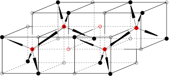
Figure 2: In the ordered low density liquid phase half of the lattice is occupied by particles. Water (filled circles) and empty sites (open circles)

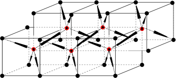
Figure 3: In the ordered high density liquid phase the lattice is fully occupied by particles.

III Non-polar solute in ALG solvent - simulations

We investigate the solution phase diagram for inert solute particles. Non-polar solutes are modeled as non-interacting hard spheres. Thus each lattice site can be empty or occupied either by a water particle or by a non-polar solute. Simulations were run as follows: solvent molecules are inserted or removed via a Grand-Canonical Monte Carlo algorithm, while a fixed number of solute particles are allowed to diffuse throughout the lattice, following the Metropolis prescription.

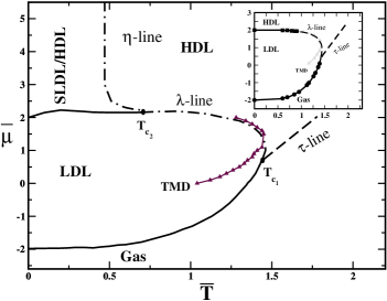
Figure 4: Chemical potential vs. temperature phase diagram for the original ALG model (inset) and ALG with 5$\%$ solute concentration.

Fig. 4 illustrates the effect on the water chemical potential versus temperature phase diagram upon the introduction of $5\%$ solute ($\rho_{solute}=0.05$ in volume fraction). At $\overline{T}=0$, the solute will be randomly distributed in the lattice. In the gas phase, because solute is inert, the semi grand-potential free energy per volume is the same as the grand potential of the solute free case, $\Omega_{gas}=0$. In the LDL phase, the solute particles occupy the empty sites which correspond to half the lattice: for 5$\%$ of solute particles, 10$\%$ of the empty sites are occupied, as illustrated in Fig. 5. Consequently, the density and the semi grand potential free energy per volume are the same as that of pure water, $\rho_{LDL}=1/2$ and $\Omega_{LDL}=\varepsilon+\gamma-1/2$ respectively. The same occurs in the phase boundary between the gas and the LDL phases at zero temperature, where $\mu_{gas-LDL}=2$. This semi grand-potential free energy per volume is only correct if the solute occupies up to 50$\%$ of the lattice.

In the HDL phase the addition of the solute changes the density and the grand potential per volume when compared with the free solute case. At zero temperature, in the solute free case, the lattice is full. As solute is added the particles replace solvent particles, changing the energy, as can be seen in Fig. 6. The solute can occupy a number of different configurations but it will choose the structure with the lowest grand potential free energy. In order to identify which is this configuration we compare two cases: all the solute forming a large cluster and the solute distributed randomly but not occupying adjacentes sites. In both cases $\rho_{HDL}=1-\rho_{solute}$ but the grand potential free energy is given respectively by $\Omega_{HDL}^{cluster}=2(3\varepsilon+2\gamma)-(4\varepsilon+2\gamma)\rho_{solute}-\mu(1-\rho_{solute})$ and by $\Omega_{HDL}^{random}=4\varepsilon+2\gamma-(6\varepsilon+2\gamma)\rho_{solute}-\mu(1-\rho_{solute})$. The last case is the scenario with lower grand potential free energy, therefore Even thought the density and the grand potential per volume is different from the free solute case, the phase boundary between the LDL and the HDL phases is given by the same value as that of pure water, namely $\mu_{LDL-HDL}=6\varepsilon+2\gamma$.

At low temperature, and $\overline{T}\neq 0$, the phase boundary between the LDL and the gas phase depends on the entropy related to the addition of the solute. In the gas phase the solute can be located at any site, while in the LDL phase the solute goes only to the empty half-lattice (see Fig. 5), which makes the entropy of the gas phase larger than the entropy of the LDL phase. This stabilizes the gas phase, moving up the chemical potential of the gas-LDL phase boundary with respect to the free solute case.

As to the LDL-HDL phase boundary at low $\overline{T}\neq 0$, distorion of bonds in either phase is small, so that at very low temperatures no entropic difference between the two phases due to the presence of the solute is observed. However, as the temperature is increased and the bond network becomes more disordered, the entropy increment caused by solute is larger in the LDL phase, thus shifting the phase boundary to higher chemical potentials.

The critical lines illustrated in Fig. 4 were obtained from the peak in the specific heat and through Binder cumulant methods [28, 29]. The critical line between the disordered phase and the HDL phase, at high temperatures ($\tau$ line), and the critical line between the HDL phase and the LDL phase ($\lambda$ line) are similar to the lines obtained in the solute free case [25]. The shift in these lines to lower temperatures is due to the higher entropy of the solute in the disordered phase.

Besides the $\lambda$’s and the $\tau$ critical lines present even if no solute is present, the system exhibits a new critical line, which we call $\eta$, at high chemical potentials. In order to inspect the new phase, we investigate the solute spatial distribution through its radial distribution function, $g(r)$, given by

$$g(\bar{r})=\frac{\langle\sum_{i=1}^{N}\sum_{j>i}^{N}{\sigma_{i}\sigma_{j}\delta[\bar{r},(\bar{r}_{i}-\bar{r}_{j})]}\rangle_{\bar{T}}}{\langle\sum_{i=1}^{N}\sum_{j>i}^{N}{\sigma_{i}\sigma_{j}\delta[\bar{r},(\bar{r}_{i}-\bar{r}_{j})]}\rangle_{\infty}}\;.$$ (3)

where the mean values denoted by $<...>_{\overline{T}}$ are obtained at constant temperature for $T=\overline{T}$ and $\overline{T}\rightarrow\infty$, and $\delta$ is the Kronecker’s delta.

Figure 7 illustrates the radial distribution function for 5$\%$ of solute for two different temperatures, $\bar{T}=0.40$ and $\bar{T}=0.70$. At high temperatures the radial distribution is characteristic of a disordered, fluid-like system, while at low temperatures solute presents an ordered (solid-like).

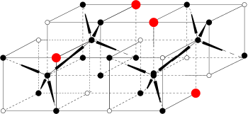
Figure 5: In the ordered low density liquid phase half of the lattice is occupied by particles and the other half contains solute.

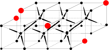
Figure 6: In the ordered high density liquid phase the lattice is completely occupied either by solute or water particles. Solutes are the bigger circles.

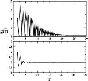
Figure 7: Solute - solute radial distribution function, g(r), for solute concentration 5$\%$. From top to bottom $\bar{T}=0.40$ and $\bar{T}=0.70$, chemical potential $\bar{\mu}=3.00$. At low temperature g(r) exhibits some structural order while at high temperature g(r) is liquid like.

To further analyse the structure of the new phase, we have measured sublattice solute and water densities. The lattice is divided into eight sub-lattices, as shown in Fig. 8. The result is shown in Fig. 9 for chemical potential fixed at $\bar{\mu}=3.00$. At high temperatures, both solvent and solute are randomly distributed, with no preferentially occupied sub-lattice. As temperature decreases and the vertical critical line is crossed, the solute particles become organized in four sub-lattices, while the solvent fills the remaining space in the eight sublattices. Therefore, the $\eta$-line separates the higher temperature homogeneous fluid phase from a dense phase in which the solute organizes itself, named SLDL/HDL phase. It is not clear, however, if inside each sub-lattice the solute particles are randomly distributed or if they cluster, forming a high density solute and a low density solute region. The behavior of the radial distribution function suggests that the later is the case. This issue is checked through the cluster approximation of the next section.

Besides the critical lines and the coexistence lines, this system with and without solute, exhibits an anomalous behavior in the density. As the temperature is decreased at constant pressure the density increases, and at very low temperatures, it decreases, thus presenting a maximum. The line of maximum density temperatures at different chemical potentials is illustrated as the line with triangles in Fig. 4. Due to the entropic effects the TMD line is located at higher temperatures when compared with the solute free case.

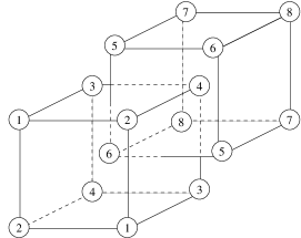
Figure 8: The eight sub-lattices division.

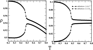
Figure 9: Density of sub-lattice as a function of temperature for chemical potential $\bar{\mu}=3.00$ and solute concentration 5$\%$. Left graph shows solvent molecules and the right one, the solute.

Having explored the effect of introducing inert solute upon the solvent chemical potential versus temperature phase diagram, we investigate the solubility of these non-interacting particles. The solubility is derived from the solute excess chemical potential which is computed through Widom’s insertion method namely

$$\mu_{ex}=-\bar{T}\ln\langle e^{-\beta e_{solute}}\rangle_{0}\;\;$$ . (4)

where $e_{solute}$ represents the energy increment due to the added solute. Note that the solutes interact only via excluded volume. In the limit of low solute concentration, the solubility is then given by

$$\Gamma=exp\left(\frac{-\mu_{ex}}{\bar{T}}\right)\;\;.$$ (5)

Figure 10 illustrates the solubility parameter $\Gamma$ as a function of temperature for solute concentrations 5$\%$ for various chemical potentials. It can be seen that the solubility exhibits a minimum for a certain range of chemical potentials. The temperatures of minimum solubility (TmS) are shown with star symbols. The TMD and the TmS lines coincide. This coincidence can be understood as follows.

The solubility is related with the amount of energy required to include a solute particle in the system. In the gas phase, as the temperature is increased, the solubility decreases because the density of the gas phase increases with temperature making more difficult to include an extra solute particle. In the HDL phase the density of solvent decreases with the increase of temperature, therefore the solubility decreases with the decrease of temperature. In the LDL phase a very interesting behavior is observed. The density, which at zero temperature is $1/2$, increases with the temperature. In this low temperature region the increase of the solvent density leaves less space for including a new solute particle and the solubility decreases. However, as the temperature is increased even further, the density of the LDL phase reaches a maximum and decreases due to entropic effects. Consequently, the solubility reaches a minimum at the maximum of solvent density, and increases with $\overline{T}$ as the system becomes less dense. The decrease of the solubility with the increase of the temperature is also observed in a minimal lattice models proposed by Widom and collaborators [30]. The focus of these different studies on the model properties have been on the relation between strength and range of the solvent mediated attraction, thus density effects, which would promote increasing solubility at larger temperatures, were left aside [31, 32].

Obviously the solubility governed solely by density effects is only possible because the solute particles, in our study, are non interacting.

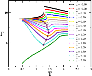
Figure 10: Solute excess chemical potential vs. temperature for different values of the water chemical potential.

IV Non-polar solute in ALG solvent - cluster variational approximation

In this section, we present results obtained from the Cluster Variational Approximation, introduced for the pure solvent version of this model by Buzano et al. [27]. The approximation is based on the assumption that an elementary tetrahedron cluster of sites, connecting the four sub-lattices (Fig. 8) is thermodynamically representative.

The energy per site is written as

$$w=\sum_{i,j,k,l}p_{ijkl}\mathcal{H}_{ijkl}\,,$$

where $p_{ijkl}$ is the joint probability for the configurations of the cluster in the four sub-lattices $1$, $2$, $3$ and $4$, and $\mathcal{H}_{ijkl}$ represents the Hamiltonian for the cluster.

For interactions restricted to nearest-neighbors the Hamiltonian $\mathcal{H}_{ijkl}$ can be decomposed in the form

$$\mathcal{H}_{ijkl}=\mathcal{H}_{ij}+\mathcal{H}_{jk}+\mathcal{H}_{kl}+\mathcal{H}_{li}\,,$$

where the pair Hamiltonian can be written as

$$\mathcal{H}_{ij}=\epsilon\sigma_{i}\sigma_{j}-\gamma\sigma_{i}\sigma_{j}h_{ij}-\frac{\mu\sigma_{i}}{4}-\frac{\nu b_{i}}{4}\,.$$

Here, $\sigma_{i}=1$ if site $i$ is occupied by a water molecule and $\sigma_{i}=0$, otherwise. The new state variable $b$ stands for solute occupation, with $b_{i}=1$ if site $i$ is occupied by a solute particle and $b_{i}=0$ otherwise. $h_{ij}$ represents bond states and is equal to $1$ if there is a bond between the two waters at sites $i$ and $j$, and equal to zero for non-bonding waters. To the parameters of the previous section, hydrogen-bond interaction $\gamma$, non-bonding penalty $\epsilon>0$ and solvent chemical potential $\mu$ we add the solute chemical potential $\nu$.

By minimizing the grand-canonical free energy

$$\frac{\omega}{T}=\sum_{i,j,k,l}p_{ijkl}\left[\frac{\mathcal{H}_{ijkl}}{T}+\ln p_{ijkl}-\frac{3}{4}\ln(p_{i}^{1}p_{j}^{2}p_{k}^{3}p_{l}^{4})\right]\,\,,$$

where $p_{i}^{1}=\sum_{jkl}p_{ijkl}$, $p_{j}^{2}=\sum_{ikl}p_{ijkl}$, $p_{k}^{3}=\sum_{ijl}p_{ijkl}$ and $p_{l}^{4}=\sum_{ijk}p_{ijkl}$. According to the natural iteration method [33], for fixed values of $T,\,\epsilon,\,\gamma,\,\mu,$ and $\nu$, one may different quantities of interest, such as solvent and solute concentrations, hydrogen bond fraction or sub-lattice densities.

In order to compare the cluster approximation results to previous simulation results, we search for the desired solute concentration ($\rho_{solute}$) by varying the corresponding solute chemical potential $\nu$. In certain ranges of the thermodynamic parameters, hysteresis loops were found.

The phase diagram for $5\%$ solute concentration ($\rho_{solute}=0.05$) is displayed in Fig. 11. It is qualitatively similar to that of simulations, and the new phase SLDL/HDL in which solute is ordered is present. In that phase, a solute droplet occupying a sub-lattice forces the neighboring solvent to order as a LDL. All other non solvent molecules are in the HDL phase. In other words, as the temperature is lowered and one crosses the fluid - SLDL/HDL line for a given value of $\mu$, a second-order phase transition takes place, and the solute, which was dispersed in the fluid phase, begins the formation of sub-lattice clusters, intercalated with LDL water. Thus, the SLDL/HDL phase is a region of coexistence between clustered and dispersed solute, or between LDL+solute and HDL-no solute.

The picture we propose for the SLDL/HDL phase is supported by behavior shown in Fig. 12, for solute density as a function of solute chemical potential $\nu$, at fixed $T$ and solvent chemical potential $\mu$, in the vicinity of the HDL - SLDL/HDL line. As $\nu$ increases, the solute density goes through a discontinuity. The diagrams show coexistence between a low density, with solute dispersed in HDL solvent, and a high density, with solute grouped in LDL solvent. Maxwell construction for the curves of Fig. 12, yield the densities of the two coexisting phases shown in Table 1. It can be seen that for $T=0.4$, for both values of the solvent chemical potential, as well as for $T=0.7$ and $\mu=2.4$, the case of $5\%$ solute density ($\rho_{solute}=0.05$) is between the low and high density limits ($\rho_{l}$ and $\rho_{h}$). The three cases correspond to points on the left of the fluid - SLDL/HDL $\eta$-line, although very near to the line in the case of $T=0.7$. On the other hand, for $\mu=3.0$ and $T=0.7$ (clearly on the right of the HDL - SLDL/HDL $\eta$-line), the low density at coexistence is $\rho_{low}=0.078$, larger than $0.05$ implying solute must be homogeneously distributed in the solution.

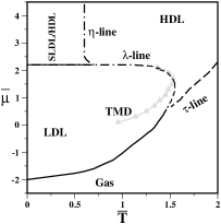
Figure 11: Solvent reduced chemical potential $\mu$ versus reduced temperature phase diagram. The Gas-LDL and LDL - SLDL/HDL coexistence phases, critical and TMD lines are shown.

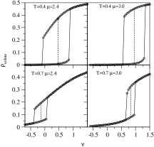
Figure 12: Solute concentration $\rho_{solute}$ as a function of the chemical potential $\nu$ for some values of temperature and water chemical potential $\mu$ near the fluid - SLDL/HDL transition line. Dashed lines give the coexistence lines.

Table 1: Solute chemical potential at the coexistence $\nu_{coex}$ and the respective concentrations of solute in both phases.

V Conclusions

In this paper we have analyzed the effect of adding non interacting solute particles to the Associating Lattice Gas Model for water. We have shown that the solute particles change the chemical potential versus temperature phase diagram substantially. In the first place, by enhancing entropic effects of the disordered and gas phases, addition of solute displaces the coexistence and critical lines accordingly. Moreover, a new phase appears, with coexistence between HDL and LDL water induced by the presence of solute. Thus, in addition to the $\lambda$ and $\tau$ critical lines present in the solute free case, a third order-disorder continuous $\eta$ transition at which the solute orders itself is present.

The solubility of this non interacting system was also computed and we have found that, as the temperature is decreased for fixed solvent chemical potential, the model solution exhibits a minimum in the solubility. The temperature of minimum of solubility coincides with the temperature of maximum density. This coincidence is due to the fact that the solute is purely hardcore. For hydrophobic or hydrophilic solutes this coincidence should to be lost.

Our results suggest a very simple mechanism for understanding the minimum of solubility in simple gases.

Acknowledgments

This work is partially supported by CNPq, Capes, INCT-FCx and Universidade Federal de Santa Catarina.

References

- Hill [1960] T. L. Hill, Statistical Thermodynamics (Addison-Wesley Pub., New York, 1960), 1st ed.
- Ivanov et al. [2005] E. V. Ivanov, E. J. Lebedeva, V. K. Abrosimov, and N. G. Ivanova, J. Struct. Chem. 46, 253 (2005).
- Ivanov and Abrosimov [2006] E. V. Ivanov and V. K. Abrosimov, Radiochemistry 48, 244 (2006).
- Filipponi et al. [1997] A. Filipponi, D. T. Bowron, C. Lobban, and J. L. Finney, Phys. Rev. Lett. 79, 1293 (1997).
- Buldyrev et al. [2007] S. V. Buldyrev, P. Kumar, P. G. Debenedetti, P. J. Rossky, and H. E. Stanley, Proc. Natl. Acad. Sci. U.S.A. 104, 20177 (2007).
- Buzano and Pretti [2003] C. Buzano and M. Pretti, J. Chem. Phys. 119, 3791 (2003).
- Chatterjee et al. [2008] S. Chatterjee, P. G. Debenedetti, F. H. Stillinger, and R. M. Lynden-Bell, J. Chem. Phys. 128, 124511 (2008).
- Waler [1964] R. Waler, Essays of natural experiments (Johnson Reprint, New York, 1964).
- Angell et al. [1976] C. A. Angell, E. D. Finch, and P. Bach, J. Chem. Phys. 65, 3063 (1976).
- Netz et al. [2001] P. A. Netz, F. W. Starr, H. E. Stanley, and M. C. Barbosa, J. Chem. Phys. 115, 344 (2001).
- Errington and Debenedetti [2001] J. R. Errington and P. G. Debenedetti, Nature (London) 409, 318 (2001).
- Buldyrev et al. [2002] S. V. Buldyrev, G. Franzese, N. Giovambattista, G. Malescio, M. R. Sadr-Lahijany, A. Scala, A. Skibinsky, and H. E. Stanley, Physica A 304, 23 (2002).
- Roberts and Debenedetti [1996] C. J. Roberts and P. G. Debenedetti, J. Chem. Phys. 105, 658 (1996).
- de Oliveira et al. [2006] A. B. de Oliveira, P. A. Netz, T. Colla, and M. C. Barbosa, J. Chem. Phys. 124, 084505 (2006).
- de Oliveira et al. [2008] A. B. de Oliveira, G. Franzese, P. A. Netz, and M. C. Barbosa, J. Chem. Phys. 128, 064901 (2008).
- Sastry et al. [1996] S. Sastry, P. G. Debenedetti, and F. Sciortino, Phys. Rev. E 53, 6144 (1996).
- Almarza et al. [2009] N. G. Almarza, J. A. Capitan, J. A. Cuesta, and E. Lomba, J. Chem. Phys 131, 124506 (2009).
- Franzese and Stanley [2007] G. Franzese and H. E. Stanley, J. Phys.: Condens. Matter 19, 205126 (2007).
- Henriques and Barbosa [2005] V. B. Henriques and M. C. Barbosa, Phys. Rev. E 71, 031504 (2005).
- Henriques et al. [2005] V. B. Henriques, N. Guissoni, M. A. Barbosa, M. Thielo, and M. C. Barbosa, Mol. Phys. 103, 3001 (2005).
- Balladares et al. [2009] A. L. Balladares, M., V. Henriques, and M. C. Barbosa, J. Phys.: Condens. Matter 19, 116105 (2009).
- Szortyka and Barbosa [2007] M. M. Szortyka and M. C. Barbosa, Physica A 380, 27 (2007).
- Girardi et al. [2007a] M. Girardi, A. L. Balladares, V. Henriques, and M. C. Barbosa, J. Chem. Phys. 126, 064503 (2007a).
- Szortyka et al. [2009] M. M. Szortyka, M. Girardi, V. Henriques, and M. C. Barbosa, J. Chem. Phys. 130, 094504 (2009).
- Szortyka et al. [2010] M. M. Szortyka, M. Girardi, V. Henriques, and M. C. Barbosa, J. Chem. Phys. 132, 134904 (2010).
- Girardi et al. [2007b] M. Girardi, M. Szortyka, and M. C. Barbosa, Physica A 386, 692 (2007b).
- Buzano et al. [2008] C. Buzano, E. De Stefanis, and M. Pretti, J. Chem. Phys. 129, 024506 (2008).
- Binder [1981] K. Binder, Z. Phys. B 43, 119 (1981).
- Landau and Binder [2003] D. P. Landau and K. Binder, A Guide to Monte Carlo Simulations in Statistical Physics (Cambridge University Press, New York, 2003), 1st ed.
- Kolomeisky and Widom [1999] A. B. Kolomeisky and B. Widom, Faraday Discussions 112, 81 (1999).
- Widom et al. [2003] B. Widom, P. Bhimalapuram, and K. Koga, Phys. Chem. Chem. Phys. 5, 3085 (2003).
- Barbosa and Widom [2010] M. A. Barbosa and B. Widom, J. Chem. Phys. 132, 214506 (2010).
- Kikuchi [1974] R. Kikuchi, J. Chem. Phys. 60, 1071 (1974).