Flow Through Randomly Curved Manifolds

Abstract

We have found that the relation between the flow through campylotic (generically curved) media, consisting of randomly located curvature perturbations, and the average Ricci scalar of the system exhibits two distinct functional expressions (hysteresis), depending on whether the typical spatial extent of the curvature perturbation lies above or below the critical value maximizing the overall Ricci curvature. Furthermore, the flow through such systems as a function of the number of curvature perturbations presents a sublinear behavior for large concentrations due to the interference between curvature perturbations that, consequently, produces a less curved space. For the purpose of this study, we have developed and validated a lattice kinetic model capable of describing fluid flow in arbitrarily curved manifolds, which allows to deal with highly complex spaces in a very compact and efficient way.

Many systems in Nature present either intrinsic spatial curvature, e.g. curved space, due to presence of stars and other interestellar media Landau and Lifshitz (1962), or geometric confinement constraining the degrees of freedom of particles moving on such media, e.g. flow on soap films Seychelles et al. (2008), solar photosphere Priest (1984), flow between two rotating cylinders and spheres Mullin and Blohm (2001); Di Prima and Swinney (1985); Bartels (1982a), to name but a few. In general, these systems force a fluid to move along non-straight trajectories (curved geodesics), leading to the upsurge of non-inertial forces. We will denote such systems as Campylotic, from the greek word $\kappa\alpha\mu\pi\acute{\upsilon}\lambda o\varsigma$ for curved, media. Due to the arbitrary trajectories that particles through a campylotic medium can take, depending on the complexity of the curved space, the flow through these media can present very unusual new transport properties. Campylotic media play a prominent role in all applications where metric curvature has a major impact on the flow structure and topology; biology, astrophysics and cosmology offering perhaps the most natural examples. Indeed, for several special cases, the flow through simple campylotic media has already been studied, e.g. Taylor-Couette flow, which was originally formulated between two concentric, rotating cylinders Mullin and Blohm (2001); Di Prima and Swinney (1985), and later extended to the case of spheres Schrauf (1986). However, beyond very simple geometries, the flow through more complicated structures, like randomly located stars or many biological systems, to the best of our knowledge, has never systematically been addressed before on quantitative grounds.

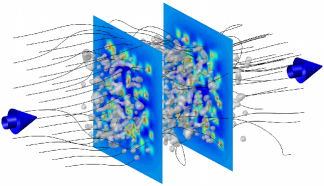
Figure 1: Streamlines of a three-dimensional fluid moving through a campylotic medium. The colors denote the Ricci scalar $R^{\prime}$ (blue and red for low and high values, respectively). The gray bubbles isosurfaces stand at $1/5$ of the maximum curvature of the system.

Since, in general, this class of flows lacks analytical solutions, their study is inherently dependent on the availability of appropriate numerical methods. Flows in complex geometries, such as cars or airplanes, make a time-honored mainstream of computational fluid dynamics (CFD), a discipline which has made tremendous progress for the last decades Hirsch and Hirsch (2007); Chen et al. (2003). However, campylotic media set a major challenge even to the most sophisticated CFD methods, because the geometrical complexity is often such to command very high spatial accuracy to resolve the most acute metric and topological features of the flow. Therefore, in this work, we also present a new lattice kinetic scheme that can handle flows in virtually arbitrary complex manifolds in a very natural and elegant way, by resorting to a covariant formulation of the lattice Boltzmann (LB) kinetic equation in general coordinates. The method is validated quantitatively for very simple campylotic media by calculating the critical Reynolds number for the onset of the Taylor-Couette instability in concentric cylinders and spheres Di Prima and Swinney (1985); Schrauf (1986); Bartels (1982a); Marcus and Tuckerman (1987), and applied to the case of two concentric tori.

In this Letter, by using the new numerical scheme, we simulate the flow through campylotic media consisting of randomly distributed spatial curvature perturbations (see Fig. 1). The flow is characterized by the number of curvature perturbations and the average Ricci scalar of the space. The campylotic media explored in this work are static, in the sense that the metric tensor and curvature are prescribed at the outset once and for all, and do not evolve self-consistently with the flow. The latter case, which is a major mainstream of current numerical relativity Baumgarte and Shapiro (1998); Schnetter et al. (2004), makes a very interesting subject for future extensions of this work.

In order to study the campylotic media, we develop a lattice kinetic approach in general geometries, taking into account the metric tensor $g_{ij}$ and the Christoffel symbols $\Gamma_{kj}^{i}$. The former characterizes the way to measure distances in space, while the latter is responsible for the non-inertial forces. The corresponding hydrodynamic equations can be obtained by replacing the partial derivatives by covariant ones, in both, the mass continuity and the momentum conservation equations. After some algebraic manipulations, the hydrodynamic equations read as follows: $\partial_{t}\rho+(\rho u^{i})_{;i}=0$, and $\partial_{t}(\rho u^{i})+T^{ij}_{;j}=0$, where the notation _;i denotes the covariant derivative with respect to spatial component $i$ (further details are given in the Supplementary Material sup ). The energy tensor $T^{ij}$ is given by, $T^{ij}=Pg^{ij}+\rho u^{i}u^{j}-\mu(g^{lj}u^{i}_{;l}+g^{il}u^{j}_{;l}+g^{ij}u^{l}_{;l})$, where $P$ is the hydrostatic pressure, $u^{i}$ the $i$-th contravariant component of the velocity, $g^{ij}$ the inverse of the metric tensor, $\rho$ is the density of the fluid, and $\mu$ is the dynamic shear viscosity.

Since lattice Boltzmann methods are based on kinetic theory, we construct our model by writing the Maxwell-Boltzmann distribution and the Boltzmann equation in general geometries. The former takes the form Love and Cianci (2011):

$$f^{\rm eq}=\frac{\sqrt{g}\rho}{\left(2\pi\theta\right)^{3/2}}\exp\left[-\frac{1}{2\theta}g_{ij}(\xi^{i}-u^{i})(\xi^{j}-u^{j})\right]\quad,$$ (1)

where $g$ is the determinant of the metric $g_{ij}$, and $\theta$ is the normalized temperature. The macroscopic and microscopic velocities, $u^{i}$ and $\xi^{i}$ are both normalized with the speed of sound $c_{s}=\sqrt{k_{B}T_{0}/m}$, $k_{B}$ being the Boltzmann constant, $T_{0}$ the typical temperature, and $m$ the mass of the particles. Note that the metric tensor appears explicitly in the distribution function, due to the fact that the kinetic energy is a quadratic function of the velocity, $u^{i}u_{i}=g_{ij}u^{i}u^{j}$. To recover the macroscopic fluid dynamic equations, we have to extract the moments from the equilibrium distribution function. The four first moments of the Maxwellian distribution function on a manifold are given by,

$$\rho=\int fd\xi\quad,\quad\rho u^{i}=\int f\xi^{i}d\xi\quad,$$ (2a)

$$\rho\theta g^{ij}+\rho u^{i}u^{j}=\int f\xi^{i}\xi^{j}d\xi\quad,$$ (2b)

$$\rho\theta(u^{i}g^{jk}+u^{j}g^{ik}+u^{k}g^{ij})+\rho u^{i}u^{j}u^{k}=\int f\xi^{i}\xi^{j}\xi^{k}d\xi.$$ (2c)

These moments are sufficient to reproduce the mass and the momentum conservation equations. Here, for simplicity we have used $d\xi$ to denote $d\xi^{1}d\xi^{2}d\xi^{3}$ and the Jacobian of the integration is already included in the Maxwell Boltzmann distribution, through the determinant term $\sqrt{g}$.

In the absence of external forces, in the standard theory of the Boltzmann equation, the single particle distribution function $f(x^{i},\xi^{i},t)$ evolves, according to the equation, $\partial_{t}f+\xi^{i}\partial_{i}f={\cal C}(f)$, where $\cal C$ is the collision term, which, using the BGK approximation, can be written as, ${\cal C}=-(1/\tau)(f-f^{\rm eq})$, with the single relaxation time $\tau$. This equation can be obtained from a more general expression, $df/dt={\cal C}(f)$, where the total time derivative now includes a streaming term in velocity space due to external forces, $\frac{df}{dt}=\partial_{t}f+\frac{dx^{i}}{dt}\partial_{i}f+\frac{dp^{i}}{dt}\partial_{p^{i}}f$, with $p^{i}$ the $i$-th contravariant component of the momentum of the particles. Using the definition of velocity, $\xi^{i}=dx^{i}/dt$, and due to the fact that the particles in our fluid move along geodesics, which implies the equation of motion

$$\frac{dp^{i}}{dt}=-\Gamma^{i}_{kl}p^{k}p^{l}\quad,$$ (3)

we can write the Boltzmann equation as Sinitsyn et al. (2011),

$$\partial_{t}f+\xi^{i}\partial_{i}f-\Gamma^{i}_{jk}\xi^{j}\xi^{k}\partial_{\xi^{i}}f={\cal C}(f)\quad,$$ (4)

where we have used the definition of the momentum, $p^{i}=m\xi^{i}$. Note that the third term of the left hand side carries all the information on non-inertial forces. Thus, all the ingredients required to model a fluid in general geometries within the Boltzmann equation are now in place. Note that the Christoffel symbols and metric tensor are arbitrary and therefore we can model the fluid flow in curved spaces, whose metric tensor is very complicated and/or only known numerically.

Since the contravariant components of the velocity are free of space-dependent metric factors, they lend themselves to standard lattice Boltzmann discretization of velocity space. All the metric and non-inertial information is conveyed into the generalized local equilibria and forcing term, respectively. These features are key to the LB formulation in general manifolds. As an additional feature, complex boundary conditions related to a specific geometry, e.g. surface of sphere, in many cases, can be treated exactly by cubic cells in the contravariant coordinate frame, thereby avoiding stair-case approximations typical of cartesian grids. The details of the discretization of this model on a lattice can be found in the Supplementary Material sup .

To provide numerical validation of our model, we study the flow through one of the simplest campylotic medium, the Taylor-Coutte instability in three different geometries, i.e. two concentric rotating cylinders, spheres and tori, respectively. Full details of the validation are given in the Supplementary Materialsup . In Figure 2, we report the critical Reynolds number as a function of the aspect ratio $\eta=a/b$, where $a$ and $b$ are the minor and major radii, respectively. As one can appreciate, for the cylindrical geometry we obtain excellent agreement with analytical theory Di Prima and Swinney (1985), and a similar match with experimental data Schrauf (1986) is found for the spherical case. We have also computed the torque coefficient, and found reasonable agreement, within a few percent, with experimental data Wimmer (1976); Bartels (1982b). For the case of two concentric rotating tori, the critical Reynolds numbers for different configurations can also be observed in Fig. 2, showing values around $10\%$ larger than for the case of cylinders. Further details can be found in the Supplementary Material sup .

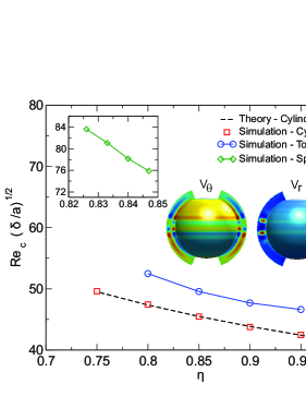
Figure 2: Critical Reynolds number $Re_{c}$, as a function of the parameter $\eta=a/b$ at the onset of the Taylor-Couette instability, for two concentric rotating cylinders (red) and tori (blue). Theoretical values for the case of the cylinders agree with Ref. Di Prima and Swinney (1985). The left inset shows the critical Reynolds number for the case of two concentric spheres, and the two colored spheres the radial and axial components of the fluid velocity for the spherical case. Blue and red colors denote low and high values, respectively.

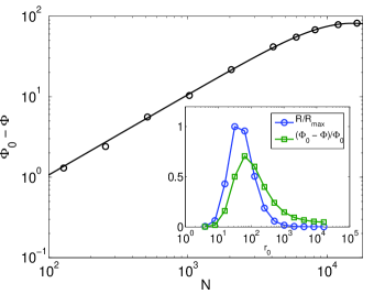
Figure 3: Flux reduction $\Phi_{0}-\Phi$ with respect to the flat case, as a function of the number of curvature perturbations for $a_{0}=0.01$ and $r_{0}=2.0$. The solid line is the analytical curve according to Eq. (5). Shown in the inset is the normalized average curvature scalar of the space, $R/R_{max}$, and the normalized reduced flux $1-\Phi_{0}/\Phi$ as a function of $r_{0}$. Both Ricci scalar and flux reduction exhibit a maximum at intermediate values of $r_{0}$. Since the two maxima are slightly shifted with respect to each other, the reduced flow as a function of $R$ exhibits an hysteresis loop (see next Figure 4).

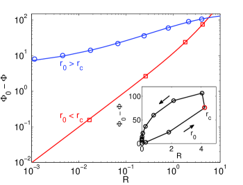
Figure 4: Flux reduction, $\Phi_{0}-\Phi$, as a function of the average curvature, $R$, for large and small values of $r_{0}$. We have fixed $a_{0}=0.00002$ and $N=1024$. The solid lines denote the analytical curves according to Eqs. (6) and  (7). The inset shows the hysteresis loop which arises by parametrizing the flux-curvature relation in terms of $r_{0}$. Here, $r_{c}$ is the radius at which the Ricci curvature attains its maximum upon increasing $r_{0}$. The lower and upper branches correspond to $r_{c}<r_{0}$ and $r_{c}>r_{0}$, respectively.

Next, we move to a genuinely campylotic medium, consisting of randomly located curvature perturbations. To this purpose, we define a coordinate system $(x,y,z)$, such that its metric tensor takes the form: $g_{ij}=\delta_{ij}(1-a_{0}\sum_{n=1}^{N}\exp(-r_{n}/r_{0}))$, where $n$ labels each local curvature perturbation located at $\vec{r}_{n}=(x_{n},y_{n},z_{n})$, $N$ is the total number of perturbations, $r_{n}=|\vec{r}_{n}|$, and $r_{0}$ characterizes the size of the deformation. Note that the coefficient $a_{0}$ can be either signed, depending on whether a positive or negative curvature is imposed, respectively. In our study, we have chosen to work with positive values of $a_{0}$, due to the analogy with a system of randomly located stars, which produce deformations in the metric tensor of spacetimeLandau and Lifshitz (1962). The Christoffel symbols are calculated numerically. The flux is calculated by the geometrical relation, $\Phi=\int_{S}\rho u^{x}\sqrt{g^{xx}g}dS$, where $S$ is the cross section at the location where the measurements are taken. Since the fluid dynamic equations only contain the metric tensor and its first derivatives (via the Christoffel symbol), and due to the fact that particles move along geodesics according to Eq. (3), it is natural to expect that the flow could be characterized by a quantity that contains the metric tensor and its first derivatives. Although the Christoffel symbols $\Gamma^{i}_{jk}$ meet this requirement, they are not components of a tensor, and therefore they are not invariant under a coordinate system transformation (physics should not depend on the choice of the coordinate system). An invariant, or tensor, that can be used to characterize the system is the Ricci tensor $R_{ik}$. In this work, we use the Ricci scalar (curvature scalar) which can be calculated from the Ricci tensor, $R_{ij}$, by contraction of the indices, $R^{\prime}=g^{ij}R_{ij}$. The relation between the metric tensor and Christoffel symbols and the Ricci tensor can be found in the Supplementary Material sup . To study this particular system, we use a lattice size $L_{x}\times L_{y}\times L_{z}$ of $128\times 64\times 64$, and $\tau=1$. All quantities will be expressed in numerical units. To drive the fluid through the medium, we add an external force along the $x$-component, which in all simulations takes the value, $f_{ext}=5\times 10^{-5}$. The flux in flat space, i.e. in the absence of curvature perturbations is denoted by $\Phi_{0}$.

Shown in Fig. 1, are the velocity streamlines, the Ricci scalar $R^{\prime}$ and the high-curvature locations, represented by gray isosurfaces. Note that the streamlines are very complex, as the flow can orbit around the spheres before continuing its trajectory Bini et al. (2009, 2012). Also we can see how the curvature perturbations interact, creating non-spherical shaped isosurfaces.

Fig. 3 shows the flux reduction $\Phi_{0}-\Phi$, as function of the number of curvature perturbations, $N$. We observe that the flux $\Phi$ decreases with $N$. This effect is due to the interplay between the longer trajectories that particles must take and the acceleration due to the non-inertial forces, see Eq. (3). Note that, in general, for systems with different configurations (e.g. negative $a_{0}$), we could expect that the combination of the two effects might lead to higher flux by increasing $N$. We also see that the flux depends linearly on $N$ for low concentration of curvature perturbations, and only sublinearly at higher concentrations. This is due to the fact that at low concentration, the average distance between curvature perturbations is large, and consequently each perturbation adds up as a single modification to the total spatial curvature. However, as the concentration is increased, the curvature perturbations start to interfere with each other and consequently the space becomes less curved (decrease of the overall Ricci curvature). The flux is found to obey the following law,

$$\Phi_{0}-\Phi=A_{1}\frac{N/N_{0}}{1+(N/N_{0})^{2}}\quad,$$ (5)

where $A_{1}=163\pm 2$ and $N_{0}=(1.54\pm 0.03)\times 10^{4}$ are fitting parameters. The parameter $N_{0}$ denotes a characteristic number of curvature perturbations, above which the sublinear behavior sets in ($N\gtrsim N_{0}$).

In the inset of Fig. 3, we observe that by fixing the number of curvature perturbations $N=1024$ and the strength $a_{0}=0.01$, and changing the range of the perturbation, $r_{0}$, the difference $\Phi_{0}-\Phi$ presents a maximum for a given $r_{0}\sim r_{c}$. Furthermore, another interesting result is that the average curvature, here defined as $R=-10^{8}<R^{\prime}>$ (where $<...>$ means average over space), shows the same qualitative behavior. Since by increasing $r_{0}$ the metric tensor components decrease monotonically, this maximum is due to the Christoffel symbols (or non-inertial forces), which can be characterized via $R$. However, the maxima are slightly shifted, due to the fact that the Ricci scalar does not uniquely determine the metric tensor and Christoffel symbols, the quantities that play a key role in the fluid dynamic equations. Taking into account this effect, we can plot the flux reduction $\Phi_{0}-\Phi$ as a function of $R$, and find that, indeed, for $r_{0}<r_{c}$, the flux decreases by increasing the average curvature $R$ with a different law than for the case of large values of $r_{0}>r_{c}$ (see inset of Fig. 4). This gives rise to a hysteresis-shaped curve, the reason for this hysteresis being that the metric tensor is different for $r_{0}<r_{c}$ and $r_{0}>r_{c}$, even if $R$ takes the same value. However, in both cases, the system shows that higher values of the average curvature $R$ always result in a lower flux. The behavior of the flux for $r_{0}<r_{c}$ is well represented by the following law:

$$\Phi_{0}-\Phi=A_{2}\frac{R}{R_{0}}\left(1+\frac{R}{R_{0}}\right)\quad,$$ (6)

and for the case of $r_{0}>r_{c}$,

$$\Phi_{0}-\Phi=A_{3}\sqrt{\frac{R}{R_{0}+R}}+\Phi^{\prime}\quad,$$ (7)

where $R_{0}=5.2\pm 0.1$, $A_{2}=50\pm 2$, $A_{3}=154\pm 4$, and $\Phi^{\prime}=5\pm 1$. The quantity $R_{0}$ is related to the maximum curvature achieved by the system and the intersection of the two laws (see Fig. 4). The other interesting quantity is $\Phi^{\prime}$, which represents the difference of flux between $r_{0}\gg r_{c}$ and $r_{0}\ll r_{c}$, when the curvature scalar becomes zero, and it is due to the fact that in both cases, although the space has no curvature, it has nonetheless different metric tensors.

Summarizing, we have explored the laws that rule the flow through campylotic media consisting of randomly distributed curvature perturbations, and shown that, for the configurations studied in this Letter, curved spaces invariably support less flux than flat spaces. Furthermore, the flux can be characterized by the Ricci scalar, a geometrical invariant that contains the metric tensor and Christoffel symbols, the quantities that appear in the fluid dynamics equations. The trajectories of the flow can become very complicated due to the total curvature of the medium, presenting, in some cases, orbits winding several times around regions with high curvature. The present method opens the possibility to apply the actual model to astrophysical systems, where the curvature of space is due to the presence of stars and other interstellar material. We have not considered time curvature, since its contribution remains sub-dominant unless mass is made extremely large.

To calculate the flux in campylotic media, we have developed a new lattice Boltzmann model to simulate fluid dynamics in general non-cartesian manifolds. The model has been successfully validated on the Taylor-Couette instability for the case of two concentric cylinders and spheres, the inner rotating with a given speed and the outer being fixed. We also studied the Taylor-Couette instability in two concentric rotating tori, finding that the critical Reynolds number for the onset of the instability is about ten percent larger than the one for the cylinder. By solving the Navier-Stokes equations in contravariant coordinates, which can be represented on a cubic lattice precisely in the format requested by the lattice Boltzmann formulation, the present model opens up the possibility to study fluid dynamics in complex manifolds by retaining the outstanding simplicity and computational efficiency of the standard lattice Boltzmann method in cartesian coordinates. The case of dynamically adaptive campylotic media, in which the metric tensor and curvature would evolve self-consistently together with the flow, makes a very interesting subject for future extensions of the present lattice kinetic method in the direction of numerical relativity Mendoza et al. (2010, 2011).

Appendix A Supplementary Material

We show the details of the new lattice kinetic model to study campylotic media, and include a respective validation by studying the Taylor-Couette instability for the case of two concentric rotating cylinders, spheres and tori. We also implement a convergence study showing that the model presents nearly second order convergence, and introduce basic relations in differential geometry like the calculation of covariant derivatives and the Ricci tensor.

Appendix B Covariant derivative and Ricci Tensor

The formulation of fluid equations in general coordinates implies the replacement of partial derivatives with the corresponding covariant ones. Given a vector $A^{i}$, the covariant derivative is defined by

$$A^{i}_{;j}=\partial_{j}A^{i}+\Gamma^{i}_{jk}A^{k}\quad,$$ (8)

where $\Gamma^{i}_{jk}$ is the Christoffel symbol associated with the curvature of the metric manifold, namely $\Gamma^{i}_{jk}=\frac{1}{2}g^{im}(\frac{\partial g_{jm}}{\partial x^{k}}+\frac{\partial g_{km}}{\partial x^{j}}-\frac{\partial g_{jk}}{\partial x^{m}})$. For an arbitrary tensor of second order, the covariant derivative is given by

$$A^{ik}_{;l}=\partial_{l}A^{ik}+\Gamma^{i}_{ml}A^{mk}+\Gamma^{k}_{ml}A^{im}\quad.$$ (9)

Here and throughout, according to Einstein’s convention, repeated indices are summed upon.

The Ricci tensor $R_{ik}$ is related with the metric tensor and Christoffel symbols by the relation,

$$R_{ik}=\frac{\partial\Gamma_{ik}^{l}}{\partial x^{l}}-\frac{\partial\Gamma_{il}^{l}}{\partial x^{k}}+\Gamma_{ik}^{l}\Gamma_{lm}^{m}-\Gamma_{il}^{m}\Gamma_{km}^{l}\quad.$$ (10)

Appendix C Tensor Hermite Polynomials

The Lattice Boltzmann formulation in general geometries makes strong reliance on Hermite expansion of the kinetic distribution function. The first three Hermite polynomials are,

$$H_{(0)}=1\quad,$$ (11a)

$$H_{(1)}^{i}=\xi^{i}\quad,$$ (11b)

$$H_{(2)}^{ij}=\xi^{i}\xi^{j}-\delta^{ij}\quad,$$ (11c)

$$H_{(3)}^{ijk}=\xi^{i}\xi^{j}\xi^{k}-(\delta^{ij}\xi^{k}+\delta^{kj}\xi^{i}+\delta^{ik}\xi^{j})\quad,$$ (11d)

where we have used the Kronecker delta $\delta^{ij}$.

Appendix D Hermite polynomials expansion

Let us expand the distribution function $f(x^{i},\xi^{i},t)$ in the form,

$$f(x^{i},\xi^{i},t)=w(\xi)\sum_{n=0}^{\infty}\frac{1}{n!}{a_{(n)}}(x^{i},t){H_{(n)}}(\xi^{i})\quad,$$ (12)

where the coefficients $a_{(n)}$ are $n$-th order space-time dependent tensors, and $H_{(n)}$ are the tensorial Hermite polynomials of $n$-th order. The weights $w(\xi)$ are defined as:

$$w(\xi)=\frac{1}{(2\pi)^{3/2}}\exp(-\xi^{2}/2)\quad.$$ (13)

The coefficients $a_{(n)}$ can be calculated with the relation,

$$a_{(n)}=\int fH_{(n)}(\xi)d\xi\quad.$$ (14)

To recover the correct hydrodynamic equations, the model must be built in such a way as to recover the first four moments, given by,

$$\rho=\int fd\xi\quad,\quad\rho u^{i}=\int f\xi^{i}d\xi\quad,$$ (15a)

$$\rho\theta g^{ij}+\rho u^{i}u^{j}=\int f\xi^{i}\xi^{j}d\xi\quad,$$ (15b)

$$\rho\theta(u^{i}g^{jk}+u^{j}g^{ik}+u^{k}g^{ij})+\rho u^{i}u^{j}u^{k}=\int f\xi^{i}\xi^{j}\xi^{k}d\xi.$$ (15c)

The fourth one ensures that the dissipation term achieves the correct form. To this purpose, we need to expand the distribution function at least up to the third order Hermite polynomial (The explicit expression of the Hermite polynomials have been given above). Thus, using Eq. (14), and replacing the Maxwell-Boltzmann distribution for a manifold, we obtain:

$$f^{\rm eq}=\frac{\sqrt{g}\rho}{\left(2\pi\theta\right)^{3/2}}\exp\left[-\frac{1}{2\theta}g_{ij}(\xi^{i}-u^{i})(\xi^{j}-u^{j})\right]\quad,$$ (16)

Next, by taking $\theta=1$ (isothermal limit), we obtain the coefficients of the expansion, as follows:

$$a_{(0)}=\rho\quad,\quad a_{(1)}^{i}=\rho u^{i}\quad,$$ (17a)

$$a_{(2)}^{ij}=g^{ij}-\delta^{ij}+\rho u^{i}u^{j}\quad,$$ (17b)

$$a_{(3)}^{ijk}=(g^{ij}-\delta^{ij})u^{k}+(g^{kj}-\delta^{kj})u^{i}+(g^{ik}-\delta^{ik})u^{j}+\rho u^{i}u^{j}u^{k}.$$ (17c)

Therefore, the truncated equilibrium distribution function up to third order, using Eq. (12), reads as follows:

$$f^{\rm eq}=w(\xi)\rho\biggl{(}\frac{5}{2} +2\xi^{i}u^{i}+\frac{1}{2}\xi^{i}g^{ij}\xi^{j}-\frac{1}{2}\xi^{i}\xi^{i}+\frac{1}{2}(\xi^{i}u^{i})^{2}-\frac{1}{2}g^{ii}-\frac{1}{2}u^{i}u^{i}+\frac{1}{6}(\xi^{i}u^{i})^{3}$$ (18)

$$-\frac{1}{2}(\xi^{i}u^{i})(u^{j}u^{j})+\frac{1}{2}(\xi^{i}u^{i})(\xi^{j}g^{jk}\xi^{k}-\xi^{j}\xi^{j})-\frac{1}{2}(\xi^{i}u^{i})(g^{jj}-3)-u^{i}g^{ij}\xi^{j}\biggr{)}\quad.$$

With this, we have expanded the equilibrium distribution function up to third order in Hermite polynomials. Next, we need to expand also the forcing term, $\Gamma^{i}_{jk}\xi^{j}\xi^{k}\partial_{\xi^{i}}f$, in the Boltzmann equation,

$$\partial_{t}f+\xi^{i}\partial_{i}f-\Gamma^{i}_{jk}\xi^{j}\xi^{k}\partial_{\xi^{i}}f={\cal C}(f)\quad,$$ (19)

Due to the fact that the distribution function can be written using Eq. (12), and invoking the properties of the Hermite polynomials,

$$wH_{(n)}^{i}=(-1)^{n}\partial_{\xi^{i}}w\quad,$$ (20)

we can write the forcing term as,

$$F^{i}\partial_{\xi^{i}}f=w\sum_{n=1}^{\infty}\frac{a_{(n-1)}F^{i}}{(n-1)!}H_{(n)}^{i}\quad,$$ (21)

where we have introduced the notation, $F^{i}=-\Gamma^{i}_{jk}\xi^{j}\xi^{k}$. Then, replacing the coefficients from Eq. (17), and the corresponding Hermite polynomials, Eq. (11), we obtain the forcing term,

$$-\Gamma^{i}_{jk}\xi^{j}\xi^{k}\partial_{\xi^{i}}f=w(\xi)\rho\biggl{(}\xi^{i}\xi^{j}\xi^{k}\Gamma^{i}_{jk} +(\xi^{l}u^{l})\xi^{i}\xi^{j}\xi^{k}\Gamma^{i}_{jk}-u^{i}\xi^{j}\xi^{k}\Gamma^{i}_{jk}$$ (22)

$$+\frac{1}{2}(g^{kl}-\delta^{kl}+u^{k}u^{l})(\xi^{k}\xi^{l}\xi^{i}\xi^{j}\xi^{m}\Gamma^{i}_{jm}-\xi^{k}\xi^{j}\xi^{i}\Gamma^{l}_{ji}-\xi^{l}\xi^{j}\xi^{i}\Gamma^{k}_{ji}-\xi^{m}\xi^{j}\xi^{i}\Gamma^{m}_{ji}\delta^{kl})\biggr{)}\quad.$$

With every term expressed as a series of Hermite polynomials, all is in place to proceed with the LB discretization according to standard Hermite-Gauss projection of the continuum Boltzmann equation.

Appendix E Lattice Discretization

In order to formulate a corresponding lattice Boltzmann model, we implement an expansion of the Maxwell-Boltzmann distribution in Hermite polynomials, so as to recover the moments of the distribution function up to third order in velocities, as it is needed to correctly reproduce the dissipation term in the hydrodynamic equations. The expansion of the Maxwell-Boltzmann distribution was introduced by Grad in his $13$ moment system Grad (1949). Since this expansion is performed in velocity space, and the metric only depends on the spatial coordinates, we expect such an expansion to preserve its validity also in the case of a general manifold. We have followed a similar procedure as the one described in Refs. Martys et al. (1998); Shan and He (1998).

For the discretization of the Maxwell Boltzmann distribution (16) and the Boltzmann equation (19), we need a discrete velocity configuration supporting the expansion up to third order in Hermite polynomials. Our scheme is based on the $D3Q41$ lattice proposed in Ref.  Chikatamarla and Karlin (2009), which corresponds to the minimum configuration supporting third-order isotropy in three spatial dimensions, along with a H-theorem for future entropic extensions Karlin et al. (1998) of the present work.

In the following, we shall use the notation $c_{\lambda}^{i}$ to denote the $i$-th contravariant component of the vector numbered $\lambda$. Thus, the discrete Boltzmann equation for our model takes the form, $f_{\lambda}(x^{i}+c^{i}_{\lambda}\delta t,t+\delta t)-f_{\lambda}(x^{i},t)=-\frac{\delta t}{\tau}(f_{\lambda}-f_{\lambda}^{\rm eq})+\delta t{\cal F}_{\lambda}$, where ${\cal F}_{\lambda}$ is the forcing term, which contains the Christoffel symbols, and $f_{\lambda}^{\rm eq}$ is the discrete form of the Maxwell-Boltzmann distribution, Eq. (16). The relevant physical information about the fluid and the geometry of the system is contained in these two terms. The macroscopic variables are obtained according to the relations, $\rho=\sum_{\lambda=0}^{41}f_{\lambda}$, $\rho u^{i}=\sum_{\lambda=0}^{41}f_{\lambda}c_{\lambda}^{i}$. The shear viscosity of the fluid can also be calculated as $\mu=\rho(\tau-1/2)c_{s}^{2}\delta t$.

In the following, we shall use the notation $c_{\lambda}^{i}$ to denote the vector number $\lambda$ and the contravariant component $i$. The cell configuration $D3Q41$ has the discrete velocity vectors: $(0,0,0)$, $(\pm 1,0,0)$, $(\pm 1,\pm 1,0)$, $(\pm 1,\pm 1,\pm 1)$, $(\pm 3,0,0)$, $(0,\pm 3,0)$, $(0,0,\pm 3)$, and $(\pm 3,\pm 3,\pm 3)$. The speed of sound for this configuration is $c_{s}^{2}=1-\sqrt{2/5}$. With this setup, and taking into account that the vectors $\xi^{i}$ and $u^{i}$ are normalized by the speed of sound, we obtain the following equilibrium distribution,

$$f_{\lambda}^{\rm eq} =w_{\lambda}\rho\biggl{(}\frac{5}{2}+2\frac{c_{\lambda}^{i}u^{i}}{c_{s}^{2}}+\frac{1}{2}\frac{c_{\lambda}^{i}g^{ij}c_{\lambda}^{j}}{c_{s}^{2}}-\frac{1}{2}\frac{c_{\lambda}^{i}c_{\lambda}^{i}}{c_{s}^{2}}$$ (23)

$$+\frac{1}{2}\frac{(c_{\lambda}^{i}u^{i})^{2}}{c_{s}^{4}}-\frac{1}{2}g^{ii}-\frac{1}{2}\frac{u^{i}u^{i}}{c_{s}^{2}}+\frac{1}{6}\frac{(c_{\lambda}^{i}u^{i})^{3}}{c_{s}^{6}}$$

$$-\frac{1}{2}\frac{(c_{\lambda}^{i}u^{i})(u^{j}u^{j})}{c_{s}^{4}}+\frac{1}{2}\frac{(c_{\lambda}^{i}u^{i})}{c_{s}^{4}}(c_{\lambda}^{j}g^{jk}c_{\lambda}^{k}-c_{\lambda}^{j}c_{\lambda}^{j})$$

$$-\frac{1}{2}\frac{(c_{\lambda}^{i}u^{i})}{c_{s}^{2}}(g^{jj}-3)-\frac{u^{i}g^{ij}c_{\lambda}^{j}}{c_{s}^{2}}\biggr{)}\quad,$$

where the weights $w_{\lambda}$ are defined as, $w_{(0,0,0)}=\frac{2}{2025}(5045-1507\sqrt{10})$, $w_{(1,0,0)}=\frac{37}{5\sqrt{10}}-\frac{91}{40}$, $w_{(1,1,0)}=\frac{1}{50}(55-17\sqrt{10})$, $w_{(1,1,1)}=\frac{1}{1600}(233\sqrt{10}-730)$, $w_{(3,0,0)}=\frac{1}{16200}(295-92\sqrt{10})$, and $w_{(3,3,3)}=\frac{1}{129600}(130-41\sqrt{10})$.

The discrete Boltzmann equation for our model takes the form,

$$f_{\lambda}(x^{i}+c^{i}_{\lambda}\delta t,t+\delta t)-f_{\lambda}(x^{i},t)=-\frac{\delta t}{\tau}(f_{\lambda}-f_{\lambda}^{\rm eq})+\delta t{\cal F}_{\lambda}\quad,$$ (24)

where we have introduced the forcing term,

$$\delta t{\cal F}_{\lambda} =w_{\lambda}\rho\Biggl{[}\frac{c_{\lambda}^{i}F_{\lambda}^{i}}{c_{s}^{2}}+\frac{(c_{\lambda}^{l}u^{l})c_{\lambda}^{i}F_{\lambda}^{i}}{c_{s}^{4}}-\frac{u^{i}F_{\lambda}^{i}}{c_{s}^{2}}$$ (25)

$$+\frac{1}{2}\left(g^{kl}-\delta^{kl}+\frac{u^{k}u^{l}}{c_{s}^{2}}\right)\Biggl{(}\frac{c_{\lambda}^{k}c_{\lambda}^{l}c_{\lambda}^{i}F_{\lambda}^{i}}{c_{s}^{4}}$$

$$-\frac{c_{\lambda}^{k}F_{\lambda}^{l}}{c_{s}^{2}}-\frac{c_{\lambda}^{l}F_{\lambda}^{k}}{c_{s}^{2}}-\frac{c_{\lambda}^{m}F_{\lambda}^{m}}{c_{s}^{2}}\delta^{kl}\Biggr{)}\Biggr{]}\quad,$$

with $F_{\lambda}^{i}=-\Gamma^{i}_{jk}\xi_{\lambda}^{j}\xi_{\lambda}^{k}$ and $\delta^{kl}$ is the Kronecker delta. In the presence of an external force $F_{\text{ext}}$, this simply extends to $F_{\lambda}^{i}\rightarrow F_{\lambda}^{i}+F^{i}_{\text{ext}\lambda}$.

In order to recover the correct macroscopic fluid equations, via a Chapman-Enskog expansion, the other moments, Eq. (15), also need to be reproduced. A straightforward calculation shows that the equilibrium distribution function $f_{\lambda}^{\rm eq}$ meets the requirement. The shear viscosity of the fluid can also be calculated as $\mu=\rho(\tau-1/2)c_{s}^{2}\delta t$. In this way one can calculate the fluid motion in spaces with arbitrary local curvatures.

Appendix F Convergence Study

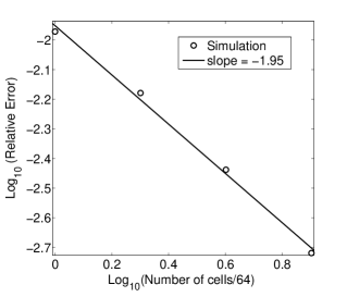
Figure 5: Relative convergence error as a function of the number of grid points. Here, the relative error is calculated by taken the mean value of the relative errors at every location grid point.

To check the convergence of the model, we simulate the Poiseuille profile for the velocity on a two-dimensional ring. For this purpose, we use the metric tensor in polar coordinates, $g_{rr}=1$, $g_{\theta\theta}=r^{2}$, and $g_{zz}=1$, where $r$ is the radial coordinate, $\theta$ is the azimuthal angle, and $z$ the axial coordinate. Thus, the non-vanishing Christoffel symbols for this metric are given by, $\Gamma^{r}_{\theta\theta}=-r$, and $\Gamma^{\theta}_{r\theta}=\Gamma^{\theta}_{\theta r}=1/r$.

Our system consists of a two-dimensional ring with inner radius $a$ and outer one $b$. On this ring, we impose a constant force $f_{a}$ in the $\theta$-direction. For the simulation we choose $\tau=0.6$. The forcing term $f_{a}$ is set to $0.05$. All numbers are expressed in numerical units. The inner radius of the ring is taken as $a=1.0$ and the outer radius as $b=1.064$. We have taken periodic boundary conditions in the direction $\theta$ and $z$, and free boundary conditions at $r=1.0$ and $r=1.064$.

To obtain a quantitative measure of the convergence we use the Richardson extrapolation method Richardson (1911); Richardson and Gaunt (1927). In this method, given any quantity $A(\delta x)$ that depends on a size step $\delta x$, we can make an estimation of order $n$ of the exact solution $A$ by using

$$A=\lim_{\delta x\rightarrow 0}A(\delta x)\approx\frac{2^{n}A\left(\frac{\delta x}{2}\right)-A(\delta x)}{2^{n}-1}+O(\delta x^{n+1})\quad,$$ (26)

with errors $O(\delta x^{n+1})$ of order $n+1$. Thus the relative error between the value $A(\delta x)$ and the “exact” solution $A$ can be calculated by

$$E_{r}(\delta x)=\left|\frac{A(\delta x)-A}{A}\right|\quad.$$ (27)

In our case, the quantity $A$ is the fluid density $\rho$, when the fluid reaches the steady state, and we set up $n=2$. Indeed, the relative error with respect to the “exact solution” decreases rapidly with increasing grid resolution (see Fig. 5) and we can see that the present scheme exhibits a near second-order convergence. This is basically in line with the convergence properties of classical LB schemes.

Appendix G Validation

To provide numerical validation of our model we study the Taylor-Couette instability, which develops between two concentric rotating cylinders. We calculate the critical Reynolds number, $Re_{c}$, which characterizes the transition between stable Couette flow and Taylor vortex flow. To this purpose, we use the metric tensor for cylindrical coordinates $(r,\theta,z)$, $g_{rr}=1$, $g_{\theta\theta}=r^{2}$, and $g_{zz}=1$, where $r$ is the radial coordinate, $\theta$ is the azimuthal angle, and $z$ the axial coordinate. Thus, the non-vanishing Christoffel symbols for this metric are given by $\Gamma^{r}_{\theta\theta}=-r$, and $\Gamma^{\theta}_{r\theta}=\Gamma^{\theta}_{\theta r}=1/r$.

In our system, the inner cylinder has radius $a$ and the outer one radius $b$. We performed several simulations, by varying the Reynolds number for different aspect ratios $\eta=a/b$. The Reynolds number, assuming that the outer cylinder is fixed, can be defined as $Re=(a\delta/\nu)d\theta/dt$ where $d\theta/dt$ is the angular speed of the inner cylinder and $\delta=b-a$. The inner radius $a$ is always set to $a=1$, and for a given value of $\eta$, the outer radius $b$ and $\delta$ are calculated. In order to vary $Re$, at fixed $\eta$, we change the angular velocity of the inner cylinder. For this simulation, we use a rectangular lattice of $128\times 1\times 256$ cells and choose $\tau=1$ (all values are given in numerical units). We use periodic boundary conditions in the $\theta$ and $z$ coordinates. At $r=a$ and $r=b$ boundaries, we have used free boundary conditions, together with a condition to impose the respective angular velocity at each boundary by evaluating the equilibrium function with those values. Note that the boundary conditions can be implemented as if they referred to a cartesian geometry, due to the use of contravariant coordinates, leading to an approximation-free representation of curved geometries. For smooth manifolds, the new scheme is about three times slower than a standard cartesian version, which is mainly due to the calculation of the metric and curvature terms, as well as to the use of third order equilibria to enhance stability. Clearly, the advantage of the present scheme lies in the treatment of complex manifolds which would require very high cartesian grid resolution.

In Fig. 2, we can observe the critical Reynolds number as a function of $\eta$, as predicted by the simulation and compared with the theoretical values from Ref. Di Prima and Swinney (1985), finding excellent agreement. We have implemented the same simulation using a lattice size $64\times 1\times 256$ cells in order to study the influence of the boundary conditions, and we found an error of around $2.5\%$ respect to the theoretical values, which is a clear evidence of the sensitivity to the boundary condition implementation. We have been able to simulate Reynolds number of around $7000$ by using $\tau=0.55$. Note that our model works in contravariant coordinates and due to the presence of a metric tensor, the time step is not necessarily unity. For this reason, even when the relaxation time is not small, the computed kinematic viscosity can achieve very small values, leading to large Reynolds numbers.

For the case of two rotating spheres, we consider the inner sphere with radius $a$ and the outer one with radius $b$. We use standard spherical coordinates $(r,\phi,\theta)$, being $r$ the radial, $\phi$ the azimuthal, and $\theta$ the polar coordinates. The non-vanishing components of the metric tensor are $g_{rr}=1$, $g_{\phi\phi}=r^{2}\sin^{2}(\theta)$, and $g_{\theta\theta}=r^{2}$. The Christoffel symbols can be calculated from the metric tensor by using standard differential geometry relations. Note that our simulation region does not include the poles because there, the determinant of the metric tensor becomes zero and therefore it is not possible to calculate its inverse. To circumvent this problem, we simulate the region $\theta\in(\pi/6,5\pi/6)$. We set $\tau=0.8$ and use a lattice of size $32\times 1\times 384$. In order to vary the Reynolds number, we change the azimuthal velocity $d\phi/dt$. The boundary conditions have been chosen periodic for the case of $\phi$, and fixed for the case of $r$ and $\theta$. In the inset (left) of Fig. 2, we show the critical Reynolds number for different configurations which is in good agreement with the experimental values given in Ref.  Schrauf (1986). In this figure, we can also observe the radial and polar components of the velocity, and see that there are two small vortices located at the equator and two large ones at high and low latitudes, in agreement with experiments and other numerical simulations Schrauf (1986); Bartels (1982a); Marcus and Tuckerman (1987).

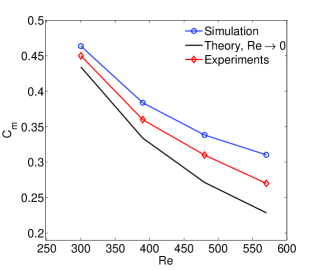
Figure 6: Torque coefficient as a function of the Reynolds number for the case of two concentric rotating spheres. The theoretical result has been taken from Ref. Wimmer (1976), and the experimental data have been collected from Ref. Wimmer (1976); Bartels (1982b).

We have also measured the torque coefficient defined by,

$$T_{r}=2\pi a^{3}\int_{0}^{\pi}\sigma_{r\phi}\sin^{2}(\theta)d\theta\quad,$$ (28)

where $\sigma_{r\phi}$ is the shear stress tensor, which in the context of lattice kinetic theory can be calculated by,

$$\sigma^{\alpha\beta}=\left(1-\frac{1}{2\tau}\right)\sum_{\lambda}^{41}(f_{\lambda}-f_{\lambda}^{\rm eq})c_{\lambda}^{\alpha}c_{\lambda}^{\beta}\quad.$$ (29)

The torque coefficient is then computed via the following relation Bartels (1982b)

$$C_{m}=\frac{T_{r}}{\frac{1}{2}\rho a^{5}\left(\frac{d\phi}{dt}\right)^{2}}\quad.$$ (30)

In Fig. 6, we show the comparison between our results, the theory for $Re\rightarrow 0$, and the experiments. We find good agreement with the experiments. The small discrepancy can be due to the approximation taken in Eq. (29) and the implementation of the boundary condition.

In order to study the Taylor-Couette instability for the case of two concentric rotating tori, which to our knowledge has never been done before, we use a lattice of size $64\times 128\times 64$ cells in the orthogonal coordinate system of the torus, $(r,u,v)$, being $r$ the radial, $u$ the axial, and $v$ the tangential coordinates. The Christoffel symbols and the components of the metric tensor can be readily calculated from differential geometry relations. The major radius of the tori has been taken as $4.0$, in numerical units. The other parameters are the same as in the previous simulations, and to vary the Reynolds number we change the tangential velocity $dv/dt$. In this case, $a$ and $b$ are the minor radii of the inner and outer tori, respectively. We use periodic boundary conditions for the coordinates $u$ and $v$, and fixed boundaries for $r$. In addition, the critical Reynolds numbers for different configurations can be observed in Fig. 2, showing values around $10\%$ larger than for the case of cylinders.

References

- Landau and Lifshitz (1962) L. D. Landau and E. M. Lifshitz, The classical theory of fields, by L. D. Landau and E. M. Lifshitz., rev. 2d ed. ed. (Pergamon Press; Addison-Wesley Pub. Co., Oxford, Reading, Mass.,, 1962) p. 404 p.
- Seychelles et al. (2008) F. Seychelles, Y. Amarouchene, M. Bessafi, and H. Kellay, Phys. Rev. Lett. 100, 144501 (2008).
- Priest (1984) E. Priest, Solar magneto-hydrodynamics, Geophysics and astrophysics monographs (D. Reidel Pub. Co., 1984).
- Mullin and Blohm (2001) T. Mullin and C. Blohm, Phys. of Fluids 13, 136 (2001).
- Di Prima and Swinney (1985) R. Di Prima and H. Swinney, in Hydrodynamic Instabilities and the Transition to Turbulence, Topics in Applied Physics, Vol. 45, edited by H. Swinney and J. Gollub (Springer Berlin / Heidelberg, 1985) pp. 139–180.
- Bartels (1982a) F. Bartels, J. Fluid Mech. 119, 1 (1982a).
- Schrauf (1986) G. Schrauf, Journal of Fluid Mechanics 166, 287 (1986).
- Hirsch and Hirsch (2007) C. Hirsch and C. Hirsch, Numerical Computation of Internal and External Flows: Fundamentals of Computational Fluid Dynamics, Butterworth Heinemann No. Bd. 1 (Butterworth-Heinemann, 2007).
- Chen et al. (2003) H. Chen, S. Kandasamy, S. Orszag, R. Shock, S. Succi, and V. Yakhot, Science 301, 633 (2003).
- Marcus and Tuckerman (1987) P. Marcus and L. Tuckerman, J. Fluid Mech. 185 (1987).
- Baumgarte and Shapiro (1998) T. W. Baumgarte and S. L. Shapiro, Phys. Rev. D 59, 024007 (1998).
- Schnetter et al. (2004) E. Schnetter, S. H. Hawley, and I. Hawke, Classical and Quantum Gravity 21, 1465 (2004).
- (13) See Supplemental Material at.
- Love and Cianci (2011) P. J. Love and D. Cianci, Philosophical Transactions of the Royal Society A: Mathematical, Physical and Engineering Sciences 369, 2362 (2011).
- Sinitsyn et al. (2011) A. Sinitsyn, E. Dulov, and V. Vedenyapin, Kinetic Boltzmann, Vlasov and Related Equations (Elsevier, 2011).
- Wimmer (1976) M. Wimmer, J. Fluid Mech. 78, 317 (1976).
- Bartels (1982b) F. Bartels, J. Fluid Mech. 119, 1 (1982b).
- Bini et al. (2009) D. Bini, R. T. Jantzen, and L. Stella, Classical and Quantum Gravity 26, 055009 (2009).
- Bini et al. (2012) D. Bini, D. Gregoris, and S. Succi, EPL (Europhysics Letters) 97, 40007 (2012).
- Mendoza et al. (2010) M. Mendoza, B. M. Boghosian, H. J. Herrmann, and S. Succi, Phys. Rev. Lett. 105, 014502 (2010).
- Mendoza et al. (2011) M. Mendoza, H. J. Herrmann, and S. Succi, Phys. Rev. Lett. 106, 156601 (2011).
- Grad (1949) H. Grad, Communications on Pure and Applied Mathematics 2, 325 (1949).
- Martys et al. (1998) N. S. Martys, X. Shan, and H. Chen, Phys. Rev. E 58, 6855 (1998).
- Shan and He (1998) X. Shan and X. He, Phys. Rev. Lett. 80, 65 (1998).
- Chikatamarla and Karlin (2009) S. S. Chikatamarla and I. V. Karlin, Phys. Rev. E 79, 046701 (2009).
- Karlin et al. (1998) I. V. Karlin, A. N. Gorban, S. Succi, and V. Boffi, Phys. Rev. Lett. 81, 6 (1998).
- Richardson (1911) L. F. Richardson, Philosophical Transactions of the Royal Society of London. Series A, Containing Papers of a Mathematical or Physical Character 210, 307 (1911).
- Richardson and Gaunt (1927) L. F. Richardson and J. A. Gaunt, Philosophical Transactions of the Royal Society of London. Series A, Containing Papers of a Mathematical or Physical Character 226, 299 (1927).