Zon-Cohen singularity and negative inverse temperature in a trapped particle limit

Abstract

We study a Brownian particle on a moving periodic potential. We focus on the statistical properties of the work done by the potential and the heat dissipated by the particle. When the period and the depth of the potential are both large, by using a boundary layer analysis, we calculate a cumulant generating function and a biased distribution function. The result allows us to understand a Zon-Cohen singularity for an extended fluctuation theorem from a view point of rare trajectories characterized by a negative inverse temperature of the biased distribution function.

I Introduction

In 1993, the fluctuation theorem was discovered Evans1993 . The theorem claims a symmetry property of the fluctuation of entropy production and provides us with a deep understanding of nonequilibrium physics Gallavotti_cohen ; Kurchan_fluctuation ; Maes_fluctuation ; Crooks_fluctuation ; Lebowitz_Spohn . The first verification of the theorem in real experiments was done by Wang et al in 2001 Wang . They used a Brownian particle dragged by an optical tweezer, and checked the fluctuation theorem for the work done by the tweezer. See also Ref. Zon-Cohen1 for the detailed analysis of the system. In the stationary state, the expectation values of the work done by the tweezer and the heat dissipated by the particle are equal to each other. However, Zon and Cohen Zon-Cohen2 ; Zon-Cohen3 predicted that the fluctuations of the work and the heat were different. They pointed out that the fluctuation theorem for the heat was modified, while the fluctuation theorem for the work was valid. They called the modified relation an extended fluctuation theorem. See Refs. Garnier ; Bonetto ; Baiesi1 ; Visco ; Harris ; Rakos ; Puglis ; Noh-Park for recent studies of the extended fluctuation theorem.

In order to examine the extended fluctuation theorem, let us consider a cumulant generating function,

$$G(h)=\frac{1}{t}\log\left\langle e^{hQ(t)}\right\rangle,$$ (1)

and a biased distribution function,

$$P_{h}(x,t)=e^{-tG(h)}\left\langle\delta(x(t)-x)e^{hQ(t)}\right\rangle,$$ (2)

where $Q(t)$ is the accumulated heat from $t=0$ to $t=t$ and $x(t)$ is the position of the particle at time $t$. The parameter $h$ is called a biasing field, because one may understand that the right-hand side of (2) is an expectation value of $\delta(x(t)-x)$ with respect to a path probability given by multiplying the original path probability by a biasing factor $e^{hQ(t)-tG(h)}$. A hardly measurable trajectory, from which we evaluate a large value of $Q(t)$, has a larger weight in (2) with $h>0$ than in the original distribution function [(2) with $h=0$]. This indicates that the biasing field is related to rare trajectories. Indeed, the large deviation theory connects rare trajectories with biasing fields more directly Dembo ; Touchette .

The extended fluctuation theorem was equivalent to a singularity of the cumulant generating function (1) Zon-Cohen2 ; Zon-Cohen3 . When $|h|$ is larger than a special value $h_{c}$, $G(h)$ becomes singular. In this paper, we call the singularity a Zon-Cohen singularity. The fact that the Zon-Cohen singularity emerges when the biasing field is larger than $h_{c}$ indicates that the singularity is related to rare trajectories. However, the relationship between the singularity and the behavior of the particle in hardly measurable trajectories is still unclear. Since the significance of fluctuation in nonequilibrium physics has been recognized recently, it is important to study the relationship using a systematic method and investigate whether the same kind of singularity occurs not only for the heat but also for the other quantities.

In this paper, we consider a Brownian particle on a moving periodic potential. The model is the overdamped case of the model studied by Lebowitz and Spohn in Ref. Lebowitz_Spohn . By using a boundary layer analysis, we calculate a cumulant generating function and a biased distribution function when the period and the depth of the potential are both large. As the result, we find that the biased distribution function becomes a canonical distribution function, where the inverse temperature is modified by $h$. When $|h|>h_{c}$, the inverse temperature becomes negative and the two limiting operations, which are the trapped particle limit and a limit of large observation time, become non-interchangeable. This non-interchangeability corresponds to the Zon-Cohen singularity. We also check a conditional distribution function given $Q(t)/t=q$. It allows us to understand how hardly measurable trajectories cause the singularity. The discussion might indicate that the same kind of singularity exists in the other quantities.

The organization of the paper is the following. In Section II, we define a model and introduce a biased process. In Section III and IV, we state main results and derive them. Finally, Section V is devoted to concluding remarks. The Boltzmann constant $k_{\rm B}$ is set to unity throughout the paper.

II Set up

II.1 Model

We consider a one-dimensional Brownian particle. The temperature of the solvent is denoted by $T$. The position of the particle is denoted by $x(t)\in\bf\mathbb{R}$. A force $-\partial U(x)/\partial x$ is exerted on the particle, where $U(x)$ is a periodic potential. The period of the potential is $2L$. That is, $U(x)$ satisfies

$$U(x)=U(x+2nL)$$ (3)

for $n=\pm 1,\pm 2,\cdots$. We move the potential with a constant velocity $v$ toward the negative direction of $x$. The motion of the particle is described by the Langevin equation

$$\dot{x}(t)=-\frac{1}{\gamma}\frac{\partial}{\partial y}U(y)\bigg{|}_{y=x(t)+vt}+\sqrt{\frac{2T}{\gamma}}\xi(t),$$ (4)

where $\xi(t)$ is the Gaussian white noise that satisfies $\left\langle\xi(t)\right\rangle=0$ and $\left\langle\xi(t)\xi(s)\right\rangle=\delta(t-s)$, and $\gamma$ is a friction constant. In order to make the analysis easy, we introduce a new variable $y(t)$ as the position of the particle measured within a reference frame that moves with the periodic potential. Concretely, $y(t)$ is defined as

$$y(t)\equiv x(t)+vt-2nL,$$ (5)

where $n$ is an integer determined by $-L\leq x(t)+vt-2nL<L$. Note that $y(t)$ is confined to $[-L,L)$. From (4), we obtain the Langevin equation for $y(t)$ as

$$\dot{y}(t)=-\frac{1}{\gamma}\frac{\partial}{\partial y}U\left(y(t)\right)+v+\sqrt{\frac{2T}{\gamma}}\xi(t).$$ (6)

This system can be realized in real experiments. See, for example, Ref. Brownian_optical_tweezer . Recently, the system has been used for experimental tests of some nonequilibrium relations Bechinger ; Ciliberto ; Toyabe .

We consider periodic potentials $U(x)$ that satisfy the following condition

$$\lim_{L\rightarrow\infty}\frac{\partial U(y)}{\partial y}\bigg{|}_{y=YL}=\infty$$ (7)

for $0<|Y|\leq 1$. A harmonic potential

$$U_{\rm harmo}(x)=\frac{1}{2}k(x-2nL)^{2},$$ (8)

and a quartic potential

$$U_{\rm quart}(x)=\frac{1}{4}k_{4}(x-2nL)^{4},$$ (9)

where $n$ is an integer determined by an inequality $-L\leq x-2nL<L$, are the examples that satisfy (7). We mention that a linear potential

$$U_{\rm linear}(x)=k_{1}|x-2nL|$$ (10)

does not satisfy (7). We display (8) in Fig. 1.

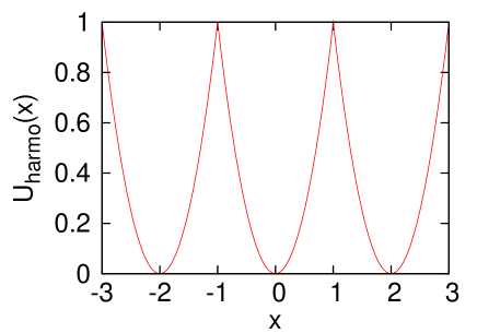
Figure 1: (Color online) A periodic potential that satisfies (7). We drew (8) by setting $k=2$ and $L=1$.

We consider the work $W(t)$ done by the periodic potential. Since the periodic potential exerts the force $-\partial U(y)/\partial y|_{y=x(t)+vt}$ on the particle and moves with the constant velocity $-v$, we find that $\dot{W}(t)$ is calculated as

$$\dot{W}(t)=(-v)\left[-\frac{\partial}{\partial y}U(y)\bigg{|}_{y=x(t)+vt}\right].$$ (11)

Next, we consider the heat $Q(t)$ dissipated by the particle. According to Sekimoto’s argument Sekimoto , the rate of the heat dissipation is evaluated as

$$\dot{Q}(t)=\dot{x}\circ\left[\gamma\dot{x}-\sqrt{2\gamma T}\xi(t)\right],$$ (12)

where the multiplication $\circ$ represents the Stratonovich interpretation Gardiner . We can immediately check that the first law of thermodynamics is satisfied. That is,

$$\int_{t_{1}}^{t_{2}}dt\left(\dot{W}(t)-\dot{Q}(t)\right)=U(x(t_{2})+vt_{2})-U(x(t_{1})+vt_{1}).$$ (13)

We also express (11) and (12) by using $y(t)$. The result is

$$\dot{W}(t)=v\frac{\partial}{\partial y}U\left(y(t)\right),$$ (14)

$$\dot{Q}(t)=\frac{1}{\gamma}\left(\frac{\partial U(y)}{\partial y}\right)^{2}-\sqrt{\frac{2T}{\gamma}}\frac{\partial U(y)}{\partial y}\circ\xi(t).$$ (15)

We denote by $\left\langle\,\right\rangle_{p}$ the expectation value over the noise $(\xi(s))_{s=0}^{\infty}$ with an initial distribution function $p(y_{0})=\left\langle\delta(y(0)-y_{0})\right\rangle$. By using the notation, we define a joint distribution function by

$$P(y_{0},y,t|p)=\left\langle\delta(y(0)-y_{0})\delta(y(t)-y)\right\rangle_{p}.$$ (16)

II.2 Biased process and cumulant generating functions

We introduce a biased process. We consider a function $f(t)$, which depends on the trajectory of the particle $(y(s))_{s=0}^{t}$. We define the expectation value of $f(t)$ in the biased process by

$$\begin{split}&\left\langle f(t)\right\rangle^{h_{w},h_{q}}_{p}\equiv e^{-tG(h_{w},h_{q},t|p)}\left\langle f(t)e^{W(t)h_{w}+Q(t)h_{q}}\right\rangle_{p},\end{split}$$ (17)

where $G(h_{w},h_{q},t|p)$ is a cumulant generating function defined by

$$G(h_{w},h_{q},t|p)=\frac{1}{t}\log\left\langle e^{W(t)h_{w}+Q(t)h_{q}}\right\rangle_{p}.$$ (18)

We note that the cumulant generating function corresponds to a thermodynamic free energy according to the thermodynamic formalism Ruelle . The two parameters $h_{w}$ and $h_{q}$ are called biasing fields. When we set $h_{w}=h_{q}=0$, the biased expectation value (17) returns to the original expectation value and the cumulant generating function (18) becomes $0$. By using (17), we define a biased joint distribution function as

$$\begin{split}&P_{h_{w},h_{q}}(y_{0},y,t|p)=\left\langle\delta(y(t)-y)\delta(y(0)-y_{0})\right\rangle^{h_{w},h_{q}}_{p}.\end{split}$$ (19)

In order to analyze the large $t$ behavior of the cumulant generating function, we define two types of functions. The first one is

$$G_{\rm scaled}(h_{w},h_{q})=\lim_{t\rightarrow\infty}G(h_{w},h_{q},t|p).$$ (20)

The second one is

$$H_{\rm ex}(h_{w},h_{q}|p)=\lim_{t\rightarrow\infty}t\left[G(h_{w},h_{q},t|p)-G_{\rm scaled}(h_{w},h_{q})\right].$$ (21)

(20) is called a scaled cumulant generating function Touchette . (21) is an excess quantity of the cumulant generating function, which was used for the calculation of an excess heat in Ref. Sagawa-Hayakawa . We call it an excess cumulant generating function. Since the excess cumulant generating function depends on the initial distribution function $p$, we explicitly indicated it in (21). By using (20) and (21), we may express $G(h_{w},h_{q},t|p)$ as

$$G(h_{w},h_{q},t|p)\simeq G_{\rm scaled}(h_{w},h_{q})+\frac{1}{t}H_{\rm ex}(h_{w},h_{q}|p).$$ (22)

We note that the difference of the left-hand side and the right-hand side of (22) is $O(e^{-at})$, where $a$ is a positive constant. See (66).

II.3 Biased distribution function and conditional distribution function

Here, we show a useful relation between the biased distribution function and a conditional distribution function. Let us consider a joint distribution function of $y(0)$, $y(t)$, and $Q(t)/t$, which is defined by

$$\begin{split}&P(y_{0},y,q,t|p)\\ &\equiv\left\langle\delta(y(0)-y_{0})\delta(y(t)-y)\delta(Q(t)/t-q)\right\rangle_{p}.\end{split}$$ (23)

By using this definition in the right-hand side of (19), we obtain a relation

$$\begin{split}&\log P_{0,h_{q}}(y_{0},y,t|p)+tG(0,h_{q},t|p)\\ &=\log\int dqP(y_{0},y,q,t|p)e^{tqh_{q}}.\end{split}$$ (24)

Then, we define a function $I(y_{0},y,q,t|p)$ by

$$I(y_{0},y,q,t|p)\equiv-\frac{1}{t}\log P(y_{0},y,q,t|p).$$ (25)

For $I(y_{0},y,q,t|p)$, we assume the following asymptotic form

$$\begin{split}&I(y_{0},y,q,t|p)=I_{0}(q)+\frac{1}{t}I_{1}(y_{0},y,q|p)+o(1/t)\end{split}$$ (26)

when $t$ is large. (26) corresponds to a large deviation property, and $I_{0}(q)$ is a large deviation function for $Q(t)/t$. By using the asymptotic form and a saddle point method, we calculate the right-hand side of (24). The result is

$$\begin{split}&t\max_{q}\left[h_{q}q-I_{0}(q)\right]-I_{1}(y_{0},y,q^{*}|p)+\frac{1}{1/t}o(1/t),\end{split}$$ (27)

where $q^{*}$ is defined as

$$q^{*}\equiv\underset{q}{\rm argmax}\left[h_{q}q-I_{0}(q)\right].$$ (28)

From (22), (24), and (27), we thus obtain

$$G_{\rm scaled}(0,h_{q})=\max_{q}\left[h_{q}q-I_{0}(q)\right],$$ (29)

and

$$\begin{split}&\log P_{0,h_{q}}(y_{0},y,t|p)+H_{\rm ex}(0,h_{q}|p)\\ &=-I_{1}(y_{0},y,q^{*}|p)+\frac{1}{1/t}o(1/t).\end{split}$$ (30)

Here, (29) is a well-known relation between a large deviation function and a scaled cumulant generating function Dembo ; Touchette . By combining (30) with (26) and noticing the normalization condition for $P_{0,h_{q}}(y_{0},y,t|p)$, we arrive at

$$P_{0,h_{q}}(y_{0},y,t|p)=\frac{P(y_{0},y,q^{*},t|p)}{P(q^{*},t|p)}+\frac{1}{1/t}o(1/t),$$ (31)

where $P(q^{*},t|p)$ is a normalization constant defined by

$$P(q^{*},t|p)\equiv\int dy_{0}dyP(y_{0},y,q^{*},t|p).$$ (32)

Since $P(q,t|p)$ is the distribution function of $Q(t)/t$, we find that the biased distribution function is nothing but the conditional distribution function of $y(0)$ and $y(t)$ given $Q(t)/t=q^{*}$.

III Results

We denote the stationary distribution function of $y$ by $p_{\rm st}^{U,v,\beta}(y)$, where the superscripts $U$, $v$, and $\beta$ indicate the periodic potential, the moving velocity of the potential, and the inverse temperature of the solvent, respectively. Then, we define a canonical distribution function $p_{\rm can}^{U,v,\beta}(y)$ by

$$p_{\rm can}^{U,v,\beta}(y)\equiv\frac{1}{Z(v,\beta)}e^{-\beta U(y)+\gamma v\beta y},$$ (33)

where $Z(v,\beta)$ is a normalization constant determined by

$$Z(v,\beta)=\int_{-L}^{L}dye^{-\beta U(y)+\gamma v\beta y}.$$ (34)

The first result is that $p_{\rm st}^{U,v,\beta}(y)$ approaches $p_{\rm can}^{U,v,\beta}(y)$ when $L$ is large:

$$p_{\rm st}^{U,v,\beta}(y)\sim p_{\rm can}^{U,v,\beta}(y)$$ (35)

for $y=YL$ ($-1<Y<1$). The definition of the symbol $\sim$ is the following. For functions $A(Y)$ and $B(Y)$, which depend on $L$, we define $A(Y)\sim B(Y)$ for $-1<Y<1$ as $\lim_{L\rightarrow\infty}(1/L)\log[A(Y)/B(Y)]=0$ for each fixed $Y$. We use the symbol $\sim$ throughout the paper.

The second result is about the scaled cumulant generating function $G_{\rm scaled}(h_{w},h_{q})$. The function always becomes a quadratic function in the limit $L\rightarrow\infty$. That is,

$$\lim_{L\rightarrow\infty}G_{\rm scaled}(h_{w},h_{q})=\gamma v^{2}(h_{w}+h_{q})+T\gamma v^{2}(h_{w}+h_{q})^{2}.$$ (36)

It should be stressed that the result is always valid whenever the periodic potential satisfies (7). From (22) and (36), we notice that

$$\begin{split}&\lim_{L\rightarrow\infty}\lim_{t\rightarrow\infty}G(h_{w},h_{q},t|p)\\ &=\gamma v^{2}(h_{w}+h_{q})+T\gamma v^{2}(h_{w}+h_{q})^{2}\end{split}$$ (37)

for any $h_{w}$ and $h_{q}$. The system under consideration was analyzed in Ref Lebowitz_Spohn by Lebowitz and Spohn. They proved the fluctuation theorem in this system. The theorem is written as

$$G_{\rm scaled}(h_{w},h_{q})=G_{\rm scaled}(-h_{w},-\beta-h_{q})|_{v\rightarrow-v},$$ (38)

where $|_{v\rightarrow-v}$ means that the sign of $v$ is reversed. We will re-derive (38) in Section IV for the sake of completeness. From (38), we obtain

$$\begin{split}&\lim_{L\rightarrow\infty}\lim_{t\rightarrow\infty}G(h_{w},h_{q},t|p)\\ &=\lim_{L\rightarrow\infty}\lim_{t\rightarrow\infty}G(-h_{w},-\beta-h_{q},t|p)|_{v\rightarrow-v},\end{split}$$ (39)

which can also be verified by using (37) directly.

Hereafter, we focus on the case in which the initial distribution function $p(y)$ is equal to a stationary distribution function $p_{\rm st}^{U,v^{\prime},\beta^{\prime}}(y)$, where $\beta^{\prime}(>0)$ and $v^{\prime}$ represent an inverse temperature and a velocity in another system. The third result is about the behavior of the biased joint distribution function $P_{h_{w},h_{q}}(y_{0},y,t|p_{\rm st}^{U,v^{\prime},\beta^{\prime}})$ when $t$ and $L$ are both large. That is,

$$\begin{split}&P_{h_{w},h_{q}}(y_{0},y,t|p_{\rm st}^{U,v^{\prime},\beta^{\prime}})\\ &\sim p_{\rm can}^{U,v_{\rm i},\beta_{\rm i}}(y_{0})p_{\rm can}^{U,v_{\rm f},\beta_{\rm f}}(y)+O(e^{-at})\end{split}$$ (40)

for $y_{0}=Y_{0}L$, $y=YL$ $(-1<Y_{0},Y<1)$ with

$$\beta_{\rm i}=\beta^{\prime}-h_{q},$$ (41)

$$v_{\rm i}=\frac{v^{\prime}\beta^{\prime}+v(h_{q}+h_{w})}{\beta^{\prime}-h_{q}},$$ (42)

$$\beta_{\rm f}=\beta+h_{q},$$ (43)

$$v_{\rm f}=\frac{v(\beta+h_{q}+h_{w})}{\beta+h_{q}}.$$ (44)

From (41) and (43), we notice that the inverse temperatures of the canonical distribution functions in (40) can become negative values. It turns out that the excess cumulant generating function has different asymptotic behaviors according to whether the inverse temperature is negative or not. This is the fourth result. Concretely, when we set $L$ to be large, the excess cumulant generating function $H_{\rm ex}(h_{w},h_{q}|p_{\rm st}^{U,v^{\prime},\beta^{\prime}})$ satisfies

$$H_{\rm ex}(h_{w},h_{q}|p_{\rm st}^{U,v^{\prime},\beta^{\prime}})=O(U(L))$$ (45)

for $\beta_{i}<0$ or $\beta_{f}<0$, and

$$H_{\rm ex}(h_{w},h_{q}|p_{\rm st}^{U,v^{\prime},\beta^{\prime}})=O(1)$$ (46)

for $\beta_{i}>0$ and $\beta_{f}>0$. From (22), (45), and (46), we find

$$\begin{split}&\lim_{t\rightarrow\infty}\lim_{L\rightarrow\infty}G(h_{w},h_{q},t|p)=\infty\end{split}$$ (47)

for $\beta_{i}<0$ or $\beta_{f}<0$, and

$$\begin{split}&\lim_{t\rightarrow\infty}\lim_{L\rightarrow\infty}G(h_{w},h_{q},t|p)=\lim_{L\rightarrow\infty}\lim_{t\rightarrow\infty}G(h_{w},h_{q},t|p)\end{split}$$ (48)

for $\beta_{i}>0$ and $\beta_{f}>0$. (48) shows that the two limiting operations, which are $L\rightarrow\infty$ and $t\rightarrow\infty$, are interchangeable and the symmetry property of the fluctuation theorem is satisfied when $\beta_{\rm i}$ and $\beta_{\rm f}$ are both positive. However, when $\beta_{\rm i}$ or $\beta_{\rm f}$ is negative, the two limiting operations become non-interchangeable. If we take $t\rightarrow\infty$ first, the cumulant generating function satisfies the fluctuation theorem (39). On the other hand, if we take $L\rightarrow\infty$ first, the cumulant generating function diverges as shown in (47). This divergence corresponds to the Zon-Cohen singularity Zon-Cohen2 ; Zon-Cohen3 .

III.1 The negative inverse temperature and the Zon-Cohen singularity

By substituting the explicit expression of the scaled cumulant generating function (38) into (28) and (29), we obtain a relation between $q^{*}$ and $h_{q}$ as

$$h_{q}=\frac{q^{*}-\gamma v^{2}}{2T\gamma v^{2}}.$$ (49)

From (31), (49), and the third result stated above, we also obtain an expression of the joint conditional distribution function. That is,

$$\frac{P(y_{0},y,q,t|p_{\rm st}^{U,v^{\prime}\beta^{\prime}})}{P(q,t|p_{\rm st}^{U,v^{\prime}\beta^{\prime}})}\sim p_{\rm can}^{U,\tilde{v}_{\rm i},\tilde{\beta}_{\rm i}}(y_{0})p_{\rm can}^{U,\tilde{v}_{\rm f},\tilde{\beta}_{\rm f}}(y)+\frac{1}{1/t}o(1/t)$$ (50)

for $y_{0}=Y_{0}L$, $y=YL$ $(-1<Y_{0},Y<1)$ with

$$\tilde{\beta}_{\rm i}=\beta^{\prime}-\frac{q-\gamma v^{2}}{2T\gamma v^{2}},$$ (51)

$$\tilde{v}_{\rm i}=\frac{v^{\prime}\beta^{\prime}+(q-\gamma v^{2})/(2T\gamma v)}{\beta^{\prime}-(q-\gamma v^{2})/(2T\gamma v^{2})},$$ (52)

$$\tilde{\beta}_{\rm f}=\beta+\frac{q-\gamma v^{2}}{2T\gamma v^{2}},$$ (53)

$$\tilde{v}_{\rm f}=v.$$ (54)

From (50), (51), and (53), we find that the particle tends to climb up the potential and to reach the top of the potential at time $t$ if $Q(t)/t$ is smaller than $-\gamma v^{2}$ [or to climb down the potential from the top at time $0$ if $Q(t)/t$ is larger than $\gamma v^{2}(2\beta^{\prime}/\beta+1)$]. Here, we show that one can obtain the singularity from these rare trajectories by using an intuitive argument.

Now, let us imagine that we measure trajectories and evaluate $G(0,h_{q},t|p_{\rm st}^{U,v^{\prime},\beta^{\prime}})$ from the trajectories. We set $t$ to be sufficiently large. Then, from (29), the trajectories required for the calculation of $G(0,h_{q},t|p_{\rm st}^{U,v^{\prime},\beta^{\prime}})$ must satisfy $Q(t)/t=q^{*}$, where $q^{*}$ was given by (49). Here, we consider the case that $\beta_{\rm f}$ is negative. It indicates that the trajectories for the calculation of $G(0,h_{q},t|p_{\rm st}^{U,v^{\prime},\beta^{\prime}})$ also satisfy $y(t)=L$ because of the negative inverse temperature. Here, by using Jensen’s inequality, we obtain

$$\begin{split}&G(h_{w},h_{q},t|p_{\rm st}^{U,v^{\prime},\beta^{\prime}})\\ &\geq\frac{1}{t}\int_{0}^{t}dt\left[h_{q}\left\langle\dot{Q}(t)\right\rangle_{p_{\rm st}^{U,v^{\prime},\beta^{\prime}}}+h_{w}\left\langle\dot{W}(t)\right\rangle_{p_{\rm st}^{U,v^{\prime},\beta^{\prime}}}\right]\\ &=-\frac{h_{q}}{t}\left\langle U(y(t))-U(y(0))\right\rangle_{p_{\rm st}^{U,v^{\prime},\beta^{\prime}}}\\ &+\frac{h_{w}+h_{q}}{t}\int_{0}^{t}dt\left\langle\dot{W}(t)\right\rangle_{p_{\rm st}^{U,v^{\prime},\beta^{\prime}}},\end{split}$$ (55)

where we used (13) at the last line. We evaluate the expectation value in the right-hand side by using the trajectories discussed above. The first term is approximated as $-h_{q}U(L)/t$. The second term can be omitted by assuming that the particle moves around the bottom of the potential during most of the time, then suddenly climbs up the potential just before the time $t$ and reaches the top of the potential at the time $t$ [$y(t)=y$]. Thus, we have

$$G(h_{w},h_{q},t|p)\gtrsim-\frac{h_{q}}{t}U(L).$$ (56)

This yields (47). We note that the case that $\beta_{\rm i}$ is negative can also be discussed by following the same argument above. The difference is that the particle goes down to the bottom of the potential from the top instead of climbing up. From these arguments, we understand how hardly measurable trajectories cause the singularity.

IV Derivation

Here, we derive the results. In the first subsection, we analyze the system with $L$ fixed. Then, in the second subsection, we perform a boundary layer analysis by considering the limit $L\rightarrow\infty$. Finally, in the third subsection, we derive the main results of the paper.

IV.1 The method of the largest eigenvalue problem and the Cole-Hopf transformation

We define an operator $\mathcal{L}_{h_{w},h_{q}}^{(y)}$ by

$$\begin{split}&\mathcal{L}^{(y)}_{h_{w},h_{q}}\cdot\varphi\\ &=-\frac{\partial}{\partial y}\left[\left(-\frac{1}{\gamma}\frac{\partial}{\partial y}U(y)+v\right)\varphi\right]+h_{w}v\left(\frac{\partial}{\partial y}U(y)\right)\varphi\\ &+h_{q}\left[\frac{1}{\gamma}\left(\frac{\partial U(y)}{\partial y}\right)^{2}-\frac{T}{\gamma}\frac{\partial^{2}}{\partial y^{2}}U(y)\right]\varphi+\frac{T}{\gamma}\frac{\partial^{2}}{\partial y^{2}}\varphi\\ &+\frac{T}{\gamma}\left(\frac{\partial U(y)}{\partial y}\right)^{2}(h_{q})^{2}\varphi+\frac{2T}{\gamma}h_{q}\frac{\partial}{\partial y}\left[\frac{\partial U(y)}{\partial y}\varphi\right].\end{split}$$ (57)

We denote the eigenfunctions of the operator by $\psi_{n}$ $(n=0,1,2,...)$ and the corresponding eigenvalues by $\mu_{n}$ $(n=0,1,2,...)$. Here, the eigenvalues are labeled such that ${\rm Re}(\mu_{n})\leq{\rm Re}(\mu_{m})$ for $n>m$, where Re$(a)$ is the real part of $a$. We also consider the adjoint operator of $\mathcal{L}_{h_{w},h_{q}}^{(y)}$, which is given by

$$\begin{split}&\mathcal{L}^{(y)\dagger}_{h_{w},h_{q}}\cdot\varphi\\ &=\left(-\frac{1}{\gamma}\frac{\partial}{\partial y}U(y)+v\right)\frac{\partial}{\partial y}\varphi+h_{w}v\left(\frac{\partial}{\partial y}U(y)\right)\varphi\\ &+h_{q}\left[\frac{1}{\gamma}\left(\frac{\partial U(y)}{\partial y}\right)^{2}-\frac{T}{\gamma}\frac{\partial^{2}}{\partial y^{2}}U(y)\right]\varphi+\frac{T}{\gamma}\frac{\partial^{2}}{\partial y^{2}}\varphi\\ &+\frac{T}{\gamma}\left(\frac{\partial U(y)}{\partial y}\right)^{2}(h_{q})^{2}\varphi-\frac{2T}{\gamma}h_{q}\left(\frac{\partial U(y)}{\partial y}\right)\frac{\partial}{\partial y}\varphi.\end{split}$$ (58)

We denote the eigenfunctions of $\mathcal{L}_{h_{w},h_{q}}^{(y)\dagger}$ by $\phi_{n}$ $(n=0,1,2,...)$ and the corresponding eigenvalues by $\nu_{n}$ $(n=0,1,2,...)$. Generally, we may set

$$\nu_{n}=(\mu_{n})^{*}.$$ (59)

The largest eigenvalues of $\mathcal{L}_{h_{w},h_{q}}^{(y)\dagger}$ and $\mathcal{L}_{h_{w},h_{q}}^{(y)}$ are real and do not degenerate, which indicates

$$\nu_{0}=\mu_{0}.$$ (60)

We also note that the eigenfunctions corresponding to the largest eigenvalue are real. These results come from the Perron-Frobenius theory. See the Appendix B of Ref. Nemoto-Sasa2 . The orthonormal conditions for the eigenfunctions are

$$\int_{-L}^{L}dy(\phi_{n}(y))^{*}\psi_{m}(y)=\delta_{n,m}$$ (61)

$(n,m=0,1,2,...)$, where $\delta_{n,m}$ is the Kronecker $\delta$.

Here, we define $q_{h_{w},h_{q}}(y_{0},y,t|p)$ by

$$q_{h_{w},h_{q}}(y_{0},y,t|p)=e^{tG(h_{w},h_{q},t|p)}P_{h_{w},h_{q}}(y_{0},y,t|p).$$ (62)

As shown in Appendix A, $\mathcal{L}_{h_{w},h_{q}}^{(y)}$ turns out to be the time evolution operator of $q_{h_{w},h_{q}}(y_{0},y,t|p)$. That is,

$$\frac{\partial}{\partial t}q_{h_{w},h_{q}}(y_{0},y,t|p)=\mathcal{L}_{h_{w},h_{q}}^{(y)}\cdot q_{h_{w},h_{q}}(y_{0},y,t|p).$$ (63)

We expand $q_{h_{w},h_{q}}(y_{0},y,t|p)$ by the eigenfunctions $(\psi_{n}(y))_{n=0}^{\infty}$ and solve the time evolution equation (63) with the initial condition $q_{h_{w},h_{q}}(y_{0},y,0|p)=p(y_{0})\delta(y-y_{0})$. The result is

$$q_{h_{w},h_{q}}(y_{0},y,t|p)=p(y_{0})\sum_{n=0}^{\infty}\left(\phi_{n}(y_{0})\right)^{*}\psi_{n}(y)e^{\mu_{n}t}.$$ (64)

Then, we consider the large $t$ behavior of $q_{h_{w},h_{q}}(y_{0},y,t|p)$. The $n=0$ term becomes dominant in the right-hand side of (64). By combining the result with the definition (62), we obtain

$$\begin{split}&P_{h_{w},h_{q}}(y_{0},y,t|p)\\ &=e^{\left(\mu_{0}-G(h_{w},h_{q},t|p)\right)t}\\ &\times\left[p(y_{0})\phi_{0}(y_{0})\psi_{0}(y)+O\left(e^{-(\mu_{0}-{\rm Re}(\mu_{1}))t}\right)\right].\end{split}$$ (65)

Furthermore, by integrating (65) with respect to $y_{0}$ and $y$, and taking the logarithm of it, we also obtain

$$\begin{split}&G(h_{w},h_{q},t|p)\\ &=\mu_{0}+\frac{1}{t}\log c_{0}\tilde{c}_{0}+O\left(e^{-(\mu_{0}-{\rm Re}(\mu_{1}))t}\right),\end{split}$$ (66)

where $c_{0}$ and $\tilde{c}_{0}$ are defined by

$$c_{0}=\int_{-L}^{L}dy\phi_{0}(y)p(y),$$ (67)

$$\tilde{c}_{0}=\int_{-L}^{L}dy\psi_{0}(y).$$ (68)

By comparing (22) with (66), we arrive at

$$G_{\rm scaled}(h_{w},h_{q})=\mu_{0},$$ (69)

$$H_{\rm ex}(h_{w},h_{q}|p)=\log c_{0}\tilde{c}_{0}.$$ (70)

Here, (69) is a well-known result Dembo ; Touchette . There have been a lot of applications in which (69) was used. See Ref. Lebowitz_Spohn , for example. The result (70) was used for the calculation of an excess heat in Ref. Sagawa-Hayakawa . From (69) and (70), we find that the expression (65) indicates that the biased joint distribution function becomes $p(y_{0})\phi_{0}(y_{0})\psi_{0}(y)e^{-H_{\rm ex}(h_{w},h_{q}|p)}$ when $t$ is large. Essentially the same result was discussed in Ref. Jack .

Next, we use the Cole-Hopf transformation in the largest eigenvalue problems $\mathcal{L}_{h_{w},h_{q}}^{(y)}$ and $\mathcal{L}_{h_{w},h_{q}}^{(y)\dagger}$, and convert the largest eigenvalue problems to a non-linear eigenvalue problem. Here, we only see the results. We define a non-linear operator $\mathcal{M}_{h,v}$ by

$$\begin{split}\mathcal{M}_{h,v}\cdot\varphi=&2Thv\frac{\partial U}{\partial y}+\frac{1}{2\gamma}\varphi^{2}\\ &+\left(-\frac{1}{\gamma}\frac{\partial U}{\partial y}+v\right)\varphi+\frac{T}{\gamma}\frac{\partial}{\partial y}\varphi.\end{split}$$ (71)

Then, we consider a non-linear eigenvalue problem

$$\mathcal{M}_{h,v}\cdot w_{h,v}=K_{h,v},$$ (72)

where the constant $K_{h,v}$ and the periodic function $w_{h,v}(y)$ are simultaneously determined from the boundary condition $w_{h,v}(-L)=w_{h,v}(L)$ and the normalization condition

$$\int_{-L}^{L}dyw_{h,v}(y)=0.$$ (73)

We introduce a potential function of $w_{h,v}(y)$ by

$$V_{h,v}(y)=-\int_{0}^{y}dzw_{h,v}(z)+\rm const.$$ (74)

From these preparations, we can show following relations

$$\phi_{0}(y)=\frac{1}{C}\exp\left[h_{q}U(y)-\frac{V_{h_{q}+h_{w},v}(y)}{2T}\right],$$ (75)

$$\psi_{0}(y)=\frac{1}{\tilde{C}}\exp\left[-\left(h_{q}+\beta\right)U(y)-\frac{V_{-\beta-h_{q}-h_{w},-v}(y)}{2T}\right],$$ (76)

$$G_{\rm scaled}(h_{w},h_{q})=\frac{K_{h_{q}+h_{w},v}}{2T},$$ (77)

where the coefficients $(C)^{*}\tilde{C}$ are determined from the normalization condition (61). The derivation of these relations is shown in Appendix B. We note that the similar arguments were presented in Refs. Nemoto-Sasa1 ; Nemoto-Sasa2 .

IV.2 Boundary layer analysis with large $L$ limit

Here, we evaluate the asymptotic behavior of $w_{h,v}(y)$ and $K_{h,v}$ when $L$ is large. In this calculation, we use the condition (7).

We use a boundary layer analysis boundarylayer in the non-linear eigenvalue problem (72). First, we define $\tilde{w}_{h,v}(Y)$ by

$$\tilde{w}_{h,v}(Y)\equiv w_{h,v}(LY),$$ (78)

where $-1\leq Y\leq 1$. By using $\tilde{w}_{h,v}(Y)$, we rewrite the left-hand side of (72) as

$$\begin{split}&2Thv\frac{\partial U(YL)}{\partial y}+\frac{1}{2\gamma}(\tilde{w}_{h,v})^{2}\\ &+\left(-\frac{1}{\gamma}\frac{\partial U(YL)}{\partial y}+v\right)\tilde{w}_{h,v}+\frac{1}{L}\frac{T}{\gamma}\frac{\partial}{\partial Y}\tilde{w}_{h,v}.\end{split}$$ (79)

Now, we treat $L^{-1}$ as a perturbation parameter. Since the coefficient in front of $\partial\tilde{w}_{h,v}/\partial Y$ is $O(L^{-1})$, we expect that there exists a certain region $I_{\rm b}$ in which $\tilde{w}_{h,v}(Y)$ changes rapidly to satisfy the periodic boundary condition and the normalization condition. That is,

$$\left|\frac{\partial\tilde{w}_{h,v}(Y)}{\partial Y}\right|\gg\left|\tilde{w}_{h,v}(Y)\right|$$ (80)

for $Y\in I_{\rm b}$. When the width of the region $I_{\rm b}$ becomes 0 in the limit $L\rightarrow\infty$, the region is called the boundary layer. We assume the existence of the boundary layer in this problem. The basic strategy of the boundary layer analysis is the following: (i) constructing the solutions inside the boundary layer (called inner solution) and outside the boundary layer (called outer solution), and (ii) asymptotically matching those solutions so that the continuity and the boundary conditions are satisfied. See Ref. boundarylayer for more details. In this paper, we consider only the outer solution and obtain the leading order of $\tilde{w}_{h,v}(Y)$ by using some assumptions. We state the result here. The derivation is shown in Appendix C.

When $L$ is large, by utilizing the condition (7), we obtain

$$\begin{split}&\tilde{w}_{h,v}(Y)\\ &=\begin{cases}2T\gamma hv\quad&-1\leq Y\leq a_{-}\\ 2\gamma\left[-v(1+Th)+(1/\gamma)\partial U(YL)/\partial y\right]\quad&a_{-}\leq Y\leq 1\end{cases}\end{split}$$ (81)

for $hv\leq 0$ and

$$\begin{split}&\tilde{w}_{h,v}(Y)\\ &=\begin{cases}2\gamma\left[-v(1+Th)+(1/\gamma)\partial U(YL)/\partial y\right]\quad&-1\leq Y\leq a_{+}\\ 2T\gamma hv\quad&a_{+}\leq Y\leq 1\end{cases}\end{split}$$ (82)

for $hv\geq 0$. The coefficients $a_{+}$ and $a_{-}$ are determined from the condition (73). That is,

$$\gamma va_{-}\left(1+2Th\right)-\gamma v+\frac{U(L)-U(a_{-}L)}{L}=0$$ (83)

and

$$\gamma va_{+}\left(1+2Th\right)+\gamma v-\frac{U(La_{+})-U(-L)}{L}=0.$$ (84)

The examples of (81) for the potentials $U_{\rm harmo}$ and $U_{\rm quart}$ are displayed as green dashed lines and purple dotted lines in Fig. 2. We also evaluate $\tilde{w}_{h,v}(Y)$ by numerically solving (72). The numerical method is the same as the one used in Ref. Nemoto-Sasa2 . The obtained lines are displayed as red solid lines in Fig. 2. The figure shows that (81) agrees with the numerical results.

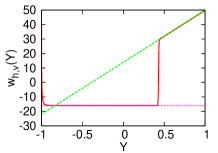
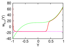
Figure 2: (Color online) $\tilde{w}_{h,v}(Y)$ for potentials $U_{\rm harmo}(y)=(k/2)y^{2}$ (left) and $U_{\rm quart}(y)=(k_{4}/4)y^{4}$ (right). Quantities are converted to dimensionless forms by setting $\gamma=T=v=1$. We fixed $k=1$, $k_{4}=1$ and $h=-8$. We set $L=18$ for $U_{\rm harmo}(y)$ and $L=3$ for $U_{\rm quart}(y)$. The green dashed lines and purple dotted lines are obtained from (81). These lines correspond to $14+36Y$ and $-16$ for $U_{\rm harmo}(y)$, and $14+54Y^{3}$ and $-16$ for $U_{\rm quart}(y)$. The red solid lines are numerical results. It can be seen that (81) agrees with the numerical results.

Next, since (72) is valid in the region that $\tilde{w}_{h,v}(Y)=2T\gamma hv$, we obtain $K_{h,v}$ as

$$K_{h,v}=2T\left(\gamma v^{2}h+T\gamma v^{2}h^{2}\right),$$ (85)

which leads to

$$G_{\rm scaled}(h_{w},h_{q})=\gamma v^{2}(h_{w}+h_{q})+T\gamma v^{2}(h_{w}+h_{q})^{2}.$$ (86)

We also check (85) by comparing it with numerical results. See Fig 3. It should be stressed that (86) is always valid under general periodic potentials, as long as the condition (7) is satisfied.

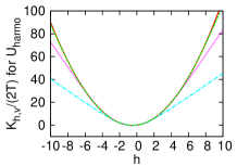
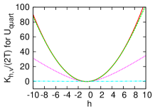
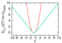
Figure 3: (Color online) $K_{h,v}/(2T)$ for potentials $U_{\rm harmo}(y)=(k/2)y^{2}$, $U_{\rm quart}(y)=(k_{4}/4)y^{4}$, and $U_{\rm linear}(y)=k_{1}|y|$. Quantities are converted to dimensionless forms by setting $\gamma=T=v=1$. We fixed $k=1$, $k_{4}=1$ and $k_{1}=1$ and numerically evaluated $K_{h,v}/(2T)$. In each figure, dashed dotted line (aqua blue), dotted line (purple), and dashed line (green) correspond to $L=6$, $L=12$ and $L=18$ for $U_{\rm harmo}$, $L=1$, $L=2$ and $L=3$ for $U_{\rm quart}$, and $L=5$, $L=25$ and $L=50$ for $U_{\rm linear}$. The red solid lines in all figures denote $h+h^{2}$, which is predicted by (85). As $L$ becomes large, $K_{h,v}$ approaches $h+h^{2}$ for $U_{\rm harmo}$ and $U_{\rm quart}$, but does not for $U_{\rm linear}$. Since $U_{\rm harmo}$ and $U_{\rm quart}$ satisfy (7) but $U_{\rm linear}$ does not, these results are consistent with our formulation.

IV.3 Derivation of the main results of the paper

From (83) and (84), we find

$$\lim_{L\rightarrow\infty}a_{\pm}=\mp 1,$$ (87)

which indicates

$$\lim_{L\rightarrow\infty}\tilde{w}_{h,v}(Y)=2T\gamma hv$$ (88)

for fixed $Y$ ($-1<Y<1$). From (88), we calculate $V_{h_{q}+h_{w},v}(y)$ and $V_{-\beta-h_{q}-h_{w},-v}(y)$ as

$$\begin{split}&\lim_{L\rightarrow\infty}V_{h_{q}+h_{w},v}(YL)/L\\ &=-\lim_{L\rightarrow\infty}\frac{1}{L}\left[\int_{0}^{YL}dzw_{h_{q}+h_{w},v}(z)+{\rm const}.\right]\\ &=-2T\gamma v(h_{q}+h_{w})Y+{\rm const}.\end{split}$$ (89)

for fixed $Y$ $(-1<Y<1)$ and

$$\begin{split}&\lim_{L\rightarrow\infty}V_{-\beta-h_{q}-h_{w},-v}(y)/L\\ &=-\lim_{L\rightarrow\infty}\frac{1}{L}\left[\int_{0}^{YL}dzw_{-\beta-h_{q}-h_{w},-v}(z)+{\rm const}.\right]\\ &=-2T\gamma v(\beta+h_{q}+h_{w})Y+{\rm const}.\end{split}$$ (90)

for fixed $Y$ $(-1<Y<1)$. By substituting these expressions into (75) and (76), we thus obtain $p(y_{0})\phi_{0}(y_{0})$ and $\psi_{0}(y)$ as

$$\begin{split}&p(y_{0})\phi_{0}(y_{0})\\ &\sim\frac{1}{C^{\prime}}\exp\left[h_{q}U(y_{0})+\log p(y_{0})+\gamma v\left(h_{q}+h_{w}\right)y_{0}\right]\end{split}$$ (91)

for $y_{0}=Y_{0}L$ $(-1<Y_{0}<1)$ and

$$\psi_{0}(y)\sim\frac{1}{\tilde{C}^{\prime}}\exp\left[-\left(\beta+h_{q}\right)U(y)+\gamma v(\beta+h_{q}+h_{w})y\right]$$ (92)

for $y=YL$ $(-1<Y<1)$, where $C^{\prime}$ and $\tilde{C}^{\prime}$ are constants determined by the normalization condition (61).

Now, we derive the results in Section III. We recall that the biased distribution function becomes the original distribution function when we set $h_{w}=h_{q}=0$. By substituting (92) into (65), we find that the stationary distribution function of this system $p_{\rm st}^{U,v,\beta}(y)$ satisfies (35).

By recalling (86), we obtain (36). Furthermore, because of (75) and (76), we have

$$\phi_{0}(y)=\psi_{0}(y)|_{(h_{w},h_{q},v)\rightarrow(-h_{w},-\beta-h_{q},-v)}.$$ (93)

Then, by utilizing (60) and (69), we obtain the fluctuation theorem for the scaled cumulant generating function as

$$G_{\rm scaled}(h_{w},h_{q})=G_{\rm scaled}(-h_{w},-\beta-h_{q})|_{v\rightarrow-v}.$$ (94)

This is (38).

Here, we consider the case in which the initial distribution function is equal to the stationary distribution function $p_{\rm st}^{U,v^{\prime},\beta^{\prime}}(y)$. By substituting (91) and (92) into (65), we obtain (40).

Finally, we derive (45) and (46). By substituting (75) and (76) into (70), and noticing the normalization condition (61), we obtain

$$\begin{split}&H_{\rm ex}(h_{w},h_{q}|p)\\ &=\log\int_{-L}^{L}dy\exp\left[h_{q}U(y)+\log p(y)-\frac{V_{h_{q}+h_{w},v}(y)}{2T}\right]\\ &+\log\int_{-L}^{L}dy\exp\left[-\left(h_{q}+\beta\right)U(y)-\frac{V_{-\beta-h_{q}-h_{w},-v}(y)}{2T}\right]\\ &-\log\int_{-L}^{L}dy\\ &\times\exp\left[-\beta U(y)-\frac{1}{2T}\left(V_{h_{q}+h_{w},v}(y)+V_{-\beta-h_{q}-h_{w},-v}(y)\right)\right].\end{split}$$ (95)

By using (89) and (90) in this expression, we obtain

$$\begin{split}H_{\rm ex}(h_{w},h_{q}|p)\simeq H+\tilde{H}+Z,\end{split}$$ (96)

where

$$\begin{split}&H\\ &\equiv\log\int_{-L}^{L}dy\exp\left[h_{q}U(y)+\log p(y)+\gamma v\left(h_{q}+h_{w}\right)y\right],\end{split}$$ (97)

$$\begin{split}&\tilde{H}\\ &\equiv\log\int_{-L}^{L}dy\exp\left[-\left(h_{q}+\beta\right)U(y)+\gamma v(\beta+h_{q}+h_{w})y\right],\end{split}$$ (98)

and

$$Z\equiv-\log\int_{-L}^{L}dy\exp\left[-\beta U(y)+\gamma v(\beta+2h_{q}+2h_{w})y\right].$$ (99)

$Z$ is always $O(1)$:

$$Z=O(1).$$ (100)

$\tilde{H}$ depends on the sign of $h_{q}+\beta$. It becomes $O(1)$ for $h_{q}+\beta>0$, but $O(U(L))$ for $h_{q}+\beta<0$. That is,

$$\tilde{H}=\begin{cases}\mathcal{O}(1)\quad&h_{q}>-\beta\\ O(U(L))\quad&h_{q}<-\beta.\end{cases}$$ (101)

$H$ depends on the initial distribution function $p(y)$. In order to see it, we introduce a parameter $\beta_{p}$

$$\beta_{p}\equiv\lim_{L\rightarrow\infty}\frac{-\log p(L)}{U(L)},$$ (102)

which can take a value from $0$ to $\infty$. It represents an effective temperature of the initial distribution function. By using $\beta_{p}$, we have

$$H=\begin{cases}O(U(L))\quad&h_{q}>\beta_{p}\\ \mathcal{O}(1)\quad&h_{q}<\beta_{p}.\end{cases}$$ (103)

From (100), (101) and (103), we arrive at the conclusion

$$H_{\rm ex}(h_{w},h_{q}|p)=\begin{cases}O(U(L))\quad&h_{q}<-\beta\\ O(1)\quad&-\beta<h_{q}<\beta_{p}\\ O(U(L))\quad&h_{q}>\beta_{p}.\end{cases}$$ (104)

By setting $p=p_{\rm st}^{U,v^{\prime},\beta^{\prime}}(y)$ in it, we obtain (45) and (46).

V Concluding remarks

In this paper, we studied the fluctuation of the work and the heat for a Brownian particle on a moving periodic potential. We considered a trapped particle limit and discussed the Zon-Cohen singularity for an extended fluctuation theorem. As the result, we found that a conditional distribution function given $Q(t)/t=q$, where $Q(t)/t$ was the rate of the heat dissipation, became a canonical distribution function. When $q$ was larger (or smaller) than a value, the inverse temperature of the canonical distribution function became negative. This indicated that the particle climbed up (climbed down) the potential. It turned out that this behavior of the particle caused the Zon-Cohen singularity.

Before ending the paper, we touch on a possibility that the singularity takes place not only for the heat but also for the other quantities. We showed that the singularity occurred because of the non-interchangeability of two types of limits. The first one was the limit of large observation time and the second one was the trapped particle limit. These limits become non-interchangeable since there exist rare trajectories in which the particle reaches the top of the potential (or climbs down the potential from the top). Aside from the heat of trapped particle systems, there might exist a system in which the same kind of singularity appears, if the system is defined by a limit and the limit is non-interchangeable with the limit of large observation time. We would like to explore such a system for a deeper understanding of fluctuation in nonequilibrium physics.

VI Acknowledgement

The author thanks S. Sasa for carefully reading this paper and providing useful comments. He also thanks S. Ito, K. Kawaguchi, M. Miyama, T. Sagawa and H. Tasaki for related discussions. This study was supported by a Grant-in-Aid for JSPS Fellows, No. 247538.

Appendix A Derivation of (63)

Here, we derive (63). We consider a joint distribution function of $y(0)$, $y(t)$, $W(t)$ and $Q(t)$, which is defined by

$$\begin{split}&P(y_{0},y,W,Q,t|p)\\ &=p(y_{0})\left\langle\delta(y(t)-y)\delta(W(t)-W)\delta(Q(t)-Q)\right\rangle_{y_{0}}.\end{split}$$ (105)

From the Langevin equations (6), (14), and (15), we have the Fokker-Planck equation for $P(y_{0},y,W,Q,t|p)$ as

$$\frac{\partial P}{\partial t}=\mathcal{L}_{\rm FP}^{(y,W,Q)}\cdot P,$$ (106)

where the Fokker-Planck operator $\mathcal{L}_{\rm FP}^{(y,W,Q)}$ is defined by

$$\begin{split}&\mathcal{L}^{(y,W,Q)}_{\rm FP}\cdot\varphi\\ &=-\frac{\partial}{\partial y}\left[\left(-\frac{1}{\gamma}\frac{\partial}{\partial y}U(y)+v\right)\varphi\right]-v\left(\frac{\partial}{\partial y}U(y)\right)\frac{\partial}{\partial W}\varphi\\ &-\left[\frac{1}{\gamma}\left(\frac{\partial U(y)}{\partial y}\right)^{2}-\frac{T}{\gamma}\frac{\partial^{2}}{\partial y^{2}}U(y)\right]\frac{\partial}{\partial Q}\varphi+\frac{T}{\gamma}\frac{\partial^{2}}{\partial y^{2}}\varphi\\ &+\frac{T}{\gamma}\left(\frac{\partial U(y)}{\partial y}\right)^{2}\frac{\partial^{2}}{\partial Q^{2}}\varphi-\frac{2T}{\gamma}\frac{\partial^{2}}{\partial Q\partial y}\left[\frac{\partial U(y)}{\partial y}\varphi\right].\end{split}$$ (107)

By multiplying (107) by $e^{Wh_{w}+Qh_{q}}$, integrating it with respect $W$ and $Q$, and noticing the definitions (19) and (62), we obtain (63).

Appendix B Derivation of (75), (76), and (77) with the Cole-Hopf transformation

Here, we derive (75), (76), and (77) from the largest eigenvalue problems of $\mathcal{L}_{h_{w},h_{q}}^{(y)}$ and $\mathcal{L}_{h_{w},h_{q}}^{(y)\dagger}$. Similar calculations were done in Refs. Nemoto-Sasa1 ; Nemoto-Sasa2 .

First, we consider the largest eigenvalue problem of $\mathcal{L}_{h_{w},h_{q}}^{(y)\dagger}$,

$$\mathcal{L}_{h_{w},h_{q}}^{(y)\dagger}\cdot\phi_{0}=\nu_{0}\phi_{0}.$$ (108)

By dividing this by $\phi_{0}$ and performing some calculations, we obtain

$$\begin{split}&\nu_{0}=(h_{q}+h_{w})v\frac{\partial U}{\partial y}+\frac{T}{\gamma}\left[\frac{\partial}{\partial y}\left(\log\phi_{0}-h_{q}U\right)\right]^{2}\\ &+\left(-\frac{1}{\gamma}\frac{\partial}{\partial y}U+v\right)\frac{\partial}{\partial y}\left(\log\phi_{0}-h_{q}U\right)\\ &+\frac{T}{\gamma}\frac{\partial}{\partial y}\left[\frac{\partial}{\partial y}\left(\log\phi_{0}-h_{q}U\right)\right].\end{split}$$ (109)

Then, we introduce a potential function $V_{0}(y)$ by

$$V_{0}(y)=-2T\left(\log\phi_{0}(y)-h_{q}U(y)\right).$$ (110)

This transformation is called the Cole-Hopf transformation. By substituting (110) into (109) and combining it with (60) and (69), we obtain

$$\mathcal{M}_{h_{w}+h_{q},v}\cdot\left(-\frac{\partial V_{0}}{\partial y}\right)=2TG_{\rm scaled}(h_{w},h_{q}),$$ (111)

Next, we consider the largest eigenvalue problem of $\mathcal{L}_{h_{w},h_{q}}^{(y)}$,

$$\mathcal{L}_{h_{w},h_{q}}^{(y)}\cdot\psi_{0}=\mu_{0}\psi_{0}.$$ (112)

We divide this by $\psi_{0}$. Then, after some calculations, we obtain

$$\begin{split}&\mu_{0}=-\left(\frac{1}{T}+h_{q}+h_{w}\right)(-v)\frac{\partial U}{\partial y}\\ &+\frac{T}{\gamma}\left[\frac{\partial}{\partial y}\left(\log\psi_{0}+\left(h_{q}+\frac{1}{T}\right)U\right)\right]^{2}\\ &+\left(-\frac{1}{\gamma}\frac{\partial U}{\partial y}-v\right)\frac{\partial}{\partial y}\left[\log\psi_{0}+\left(h_{q}+\frac{1}{T}\right)U\right]\\ &+\frac{T}{\gamma}\frac{\partial}{\partial y}\left[\frac{\partial}{\partial y}\left(\log\psi_{0}+\left(h_{q}+\frac{1}{T}\right)U\right)\right].\end{split}$$ (113)

Thus, by defining

$$\tilde{V}_{0}(y)=-2T\left[\log\psi_{0}(y)+\left(h_{q}+\frac{1}{T}\right)U(y)\right],$$ (114)

substituting it into (113), and combining it with (69), we obtain

$$\mathcal{M}_{-\beta-h_{w}-h_{q},-v}\cdot\left(-\frac{\partial\tilde{V}_{0}}{\partial y}\right)=2TG_{\rm scaled}(h_{w},h_{q}),$$ (115)

Note that the sign of the velocity in the left-hand side of (115) is reversed. This reflects a reversed protocol of moving the periodic potential.

From (110), (111), (114), and (115), we obtain (75), (76), and (77). We mention that the uniqueness of the solution of the non-linear eigenvalue problem (72) is guaranteed by the Perron-Frobenius theory, because (72) can be rewritten as the same form as (108) by following the same calculation from (111) to (108).

Appendix C Derivation of (81) and (82) by using Boundary layer analysis

Here, we derive (81) and (82). We consider the outer solution $\tilde{w}_{h,v}^{{\rm o}}(Y)$ of (72), which satisfies

$$\left|\frac{\partial\tilde{w}_{h,v}^{{\rm o}}(Y)}{\partial Y}\right|\approx\left|\tilde{w}_{h,v}^{{\rm o}}(Y)\right|,$$ (116)

where $\approx$ means that the left-hand side and the right-hand side are of the same order of magnitude. We recall that (72) is a quadratic equation for $\tilde{w}_{h,v}(Y)$. Then, by solving this, we obtain the following identity:

$$\begin{split}\tilde{w}_{h,v}(Y)&=\gamma\Bigg{[}-v+\frac{1}{\gamma}\frac{\partial U(YL)}{\partial y}\\ &\qquad\pm\left|v(1+2Th)-\frac{1}{\gamma}\frac{\partial U(YL)}{\partial y}\right|\sqrt{1+R(Y)}\Bigg{]},\end{split}$$ (117)

where $R(Y)$ is defined by

$$\begin{split}R(Y)\equiv&\frac{-v^{2}4Th(1+Th)+2K_{h,v}/\gamma}{\left[v(1+2Th)-(1/\gamma)\partial U(YL)/\partial y\right]^{2}}\\ &+\frac{-2T/(\gamma^{2}L)\partial\tilde{w}_{h,v}/\partial Y}{\left[v(1+2Th)-(1/\gamma)\partial U(YL)/\partial y\right]^{2}}.\end{split}$$ (118)

Here, we set $\tilde{w}_{h,v}(Y)=\tilde{w}_{h,v}^{{\rm o}}(Y)$ in the right-hand side of (118). From (116) and (7), we find that the second term of it is negligible. Then, we assume that $K_{h,v}$, which is equal to $2TG_{\rm scaled}(h_{w},h_{q})|_{h_{w}+h_{q}=h}$, is $O(1)$. By combining this assumption with (7), we also find that the first term of (118) is negligible. Therefore, we omit the term $R(Y)$ in (117). The result leads to an expression of the outer solution $\tilde{w}_{h,v}^{{\rm o}}(Y)$,

$$\begin{split}&\tilde{w}_{h,v}^{{\rm o}}(Y)=\begin{cases}2T\gamma hv\\ 2\gamma\left[-v(1+Th)+(1/\gamma)\partial U(YL)/\partial y\right].\end{cases}\end{split}$$ (119)

Now, in order to connect these two solutions, we use following assumptions. First, we may treat the boundary layer of this problem as a connection between these two outer solutions. Second, the number of the connecting points should be minimized. Third, the one of the connecting points must be $Y=\pm 1$ Commentappendix . By combining these assumptions with the normalization condition (73), we can uniquely determine the solution $\tilde{w}_{h,v}(Y)$ as (81) and (82).

References

- (1) D. J. Evans, E. G. D. Cohen, and G. P. Morriss, Phys. Rev. Lett. 71, 2401 (1993).
- (2) G. Gallavotti and E. G. D. Cohen, Phys. Rev. Lett. 74, 2694 (1995).
- (3) J. Kurchan, J. Phys. A 31, 3719 (1998).
- (4) C. Maes, J. Stat. Phys. 95, 367 (1999).
- (5) G. E. Crooks, Phys. Rev. E 60, 2721 (1999).
- (6) J. L. Lebowitz and H. Spohn, J. Stat. Phys. 95, 333 (1999).
- (7) G. M. Wang, E. M. Sevick, E. Mittag, D. J. Searles, and D. J. Evans, Phys. Rev. Lett. 89, 050601 (2002).
- (8) R. van Zon and E. G. D. Cohen, Phys. Rev. E 67, 046102 (2003).
- (9) R. van Zon and E. G. D. Cohen, Phys. Rev. Lett. 91, 110601 (2003).
- (10) R. van Zon and E. G. D. Cohen, Phys. Rev. E 69, 056121 (2004).
- (11) N. Garnier and S. Ciliberto, Phys. Rev. E 71, 060101(R) (2005).
- (12) F. Bonetto, G. Gallavotti, A. Giuliani, and F. Zamponi, J. Stat. Phys. 123, 39 (2006).
- (13) M. Baiesi, T. Jacobs, C. Maes, and N. S. Skantzos, Phys. Rev. E 74, 021111 (2006).
- (14) P. Visco, J. Stat. Mech. (2006) P06006.
- (15) R. J. Harris, A. Rákos and G. M. Schűtz, Europhys. Lett. 75, 227 (2006).
- (16) A. Rákos and R. J. Harris, J. Stat. Mech. (2008) P05005.
- (17) A. Puglisi, L. Rondoni and A. Vulpiani, J. Stat. Mech. (2006) P08010.
- (18) J. D. Noh and J.-M. Park, Phys. Rev. Lett. 108, 240603 (2012).
- (19) H. Touchette, Phys. Rep. 478, 1, (2009).
- (20) A. Dembo and O. Zeitouni, Large Deviations Techniques and Applications (Springer, New York, 1998).
- (21) L. P. Faucheux, G. Stolovitzky, and A. Libchaber, Phys. Rev. E, 51, 5239 (1995).
- (22) V. Blickle, T. Speck, C. Lutz, U. Seifert, and C. Bechinger, Phys. Rev. Lett. 98, 210601 (2007).
- (23) J. R. Gomez-Solano, A. Petrosyan, S. Ciliberto, R. Chetrite, and K. Gawȩdzki, Phys. Rev. Lett. 103, 040601 (2009).
- (24) S. Toyabe, T. Sagawa, M. Ueda, E. Muneyuki, and M. Sano, Nat. Phys. 6, 988 (2010).
- (25) K. Sekimoto, Stochastic Energetics Lecture Notes in Physics, Vol. 799 (Springer, Berlin, 2010).
- (26) C. W. Gardiner, Handbook of Stochastic Methods for Physics, Chemistry, and the Natural Sciences (Springer-Verlag, Berlin, 1983).
- (27) D. Ruelle, Thermodynamic Formalism (Addison-Wesley, Reading, 1978).
- (28) T. Sagawa and H. Hayakawa, Phys. Rev. E 84, 051110 (2011).
- (29) T. Nemoto and S.-i. Sasa, Phys. Rev. E 84, 061113 (2011).
- (30) R. Jack and P. Sollich, Prog. Theor. Phys. Supp. 184, 304 (2010).
- (31) T. Nemoto and S.-i. Sasa, Phys. Rev. E 83, 030105(R) (2011).
- (32) C. M. Bender and S. A. Orszag, Advanced Mathematical Methods for Scientists and Engineers (McGraw-Hill, New York,1978).
- (33) The location of the point might depend on where the derivative of the potential has discontinuity. In the cases of and , the derivatives of have discontinuities at and the one of the connecting point is located at .