The Redshift Evolution of the Relation between Stellar Mass,
Star Formation Rate, and Gas Metallicity of Galaxies

Abstract

We investigate the relation between stellar mass ($M_{\star}$), star formation rate (SFR), and metallicity ($Z$) of galaxies, so called the fundamental metallicity relation, in the galaxy sample of the Sloan Digital Sky Survey Data Release 7. We separate the galaxies into narrow redshift bins and compare the relation at different redshifts, and find statistically significant ($>99$%) evolution. We test various observational effects that might cause seeming $Z$ evolution, and find it difficult to explain the evolution of the relation only by the observational effects. In the current sample of low redshift galaxies, galaxies with different $M_{\star}$ and SFR are sampled from different redshifts, and there is degeneracy between $M_{\star}$/SFR and redshift. Hence it is not straightforward to distinguish a relation between $Z$ and SFR from a relation between $Z$ and redshift. The separation of the intrinsic relation from the redshift evolution effect is a crucial issue to understand evolution of galaxies.

1. INTRODUCTION

Stellar mass ($M_{\star}$), star formation rate (SFR), and metallicity ($Z$) of galaxies are essential parameters to understand evolution of galaxies (e.g., Kauffmann et al., 2003a; Brinchmann et al., 2004; Tremonti et al., 2004; Salim et al., 2007). The relation between $M_{\star}$ and $Z$ has been studied at various redshifts (e.g., Tremonti et al., 2004; Savaglio et al., 2005; Erb et al., 2006; Liu et al., 2008). Ellison et al. (2008) added the 3rd parameter to the $M_{\star}$–$Z$ relation, and found the 3D correlation between $M_{\star}$, SFR, and $Z$ of field star forming galaxies at low redshifts ($z\sim 0.1$) in the Sloan Digital Sky Survey (SDSS) galaxy sample. Recently, Mannucci et al. (2010, hereafter M10) and Lara-López et al. (2010) showed that high redshift galaxies ($z\lesssim 3$) agree with the extrapolation of the $M_{\star}$–SFR–$Z$ relation defined at low redshifts (so called the fundamental metallicity relation).

The no-evolution of the $M_{\star}$–SFR–$Z$ relation with redshift suggests existence of a physical process which affects evolution of galaxies in the wide range of redshift behind the relation. Some models are already proposed to explain the origin of the $M_{\star}$–SFR–$Z$ relation (Davé et al., 2012; Dayal et al., 2012; Yates et al., 2012)

Although the correlation between $M_{\star}$, SFR, and $Z$ is tested at various redshifts (M10; Lara-López et al., 2010; Richard et al., 2011; Yabe et al., 2011; Nakajima et al., 2012; Cresci et al., 2012; Wuyts et al., 2012), galaxies observed at different redshifts typically have different $M_{\star}$ and SFR. Hence the comparison of galaxy metallicities at different redshifts in a same range of $M_{\star}$ and SFR is hardly done. Thus it is currently difficult to distinguish a fundamental relation between $M_{\star}$, SFR, and $Z$ that stands in wide range of redshift, from a series of the $M_{\star}$–$Z$ relations at various redshifts.

In this study, we separate the low redshift galaxy sample ($z<0.3$) in which the $M_{\star}$–SFR–$Z$ relation is defined into narrow redshift bins, and investigate redshift evolution of the relation. Throughout this paper, we assume the fiducial cosmology with $\Omega_{\Lambda}=0.7$, $\Omega_{m}=0.3$, and $H_{0}=$ 70 km s^-1 Mpc^-1.

2. THE GALAXY SAMPLE

We draw galaxies for our analysis from the SDSS MPA-JHU Data Release 7 catalog (hereafter the MPA-JHU catalog), with similar selection criteria to that in M10 as follows. We select galaxies (1) at redshifts between 0.07 and 0.3, (2) the signal-to-noise ratio (S/N) of H$\alpha$ line $>25$, (3) $A_{V}<2.5$, (4) H$\alpha$ to H$\beta$ flux ratio (H$\alpha$/H$\beta$) $>2.5$, and (5) not strongly affected by active galactic nuclei (AGN) according to Kauffmann et al. (2003b). These selection criteria are identical to those in M10.

The target galaxy selection method for the spectroscopic observation in the SDSS provides highly uniform and complete sample of galaxies above applied magnitude limit that is $r$-band Petrosian magnitude $m_{r,{\rm Pet}}\leq 17.77$ (Strauss et al., 2002). However, galaxies fainter than this limit which have been selected by different selection methods (e.g. luminous red galaxy sample, Eisenstein et al., 2001) are also included in the MPA-JHU catalog. To avoid possible selection effect in those galaxies, we impose following selection criteria in addition to the M10 criteria. Galaxies in our sample (6) have $m_{r,{\rm Pet}}\leq 17.77$, (7) are selected for spectroscopic targets as galaxy candidates (Stoughton et al., 2002), and (8) spectroscopically confirmed as galaxies by the SDSS spectroscopic pipeline (see the SDSS DR7 website for detail). Finally $\sim 110000$ galaxies are left in our sample. We note that $\sim$ 90% of the galaxies in our sample is at $z<0.15$, although we collect galaxies at redshifts up to 0.3.

We use $M_{\star}$ and SFR of galaxies listed in the MPA-JHU catalog (Kauffmann et al., 2003a; Brinchmann et al., 2004; Salim et al., 2007), and measure metallicity of the galaxies using empirical method by Maiolino et al. (2008). Following M10, we use $R_{23}=$ ([OII]$\lambda$3727+[OIII]$\lambda$4958,5007)/H$\beta$, and [NII]$\lambda$6584/H$\alpha$ as the indicators of metallicity. The line flux ratios are corrected for extinctions using H$\alpha$/H$\beta$ and the extinction curve given by Cardelli et al. (1989). When both indicators are applicable to a galaxy, we use mean of the 12 + log(O/H) values given by the two indicators, as far as the two values agree with each other within 0.25 dex. When the two indicators disagree, we remove the galaxy from our sample. Only 3% of galaxies in our sample is rejected here, similarly to the case in M10.

3. CORRELATION OF SFR AND METALLICITY

Figure 1.— The correlation between SFR and $Z$ of the galaxies with log $M_{\star}/M_{\odot}=11.0\pm 0.05$, $10.75\pm 0.05$, $10.5\pm 0.05$, $10.25\pm 0.05$, and $10.0\pm 0.05$ from top to bottom, respectively. The data points connected with solid lines (black) represents the median metallicity of the galaxies in the whole range of redshift $0.07<z<0.3$ in each SFR bin. The data points connected with dashed (blue) and dotted (red) lines represent the median metallicities of the low and high redshift samples. The vertical error bars represent the error of mean of the metallicity distribution in each bin (the scatter of the sample divided by the square root of the sample number). The horizontal error bars represent the width of the SFR bin. The low and high redshift data points are slightly shifted sideway for visibility. The grey dots represent individual galaxies. A colored version of the figure is available in the online journal.

We show the correlation between SFR and metallicity of the galaxies in mass ranges log $M_{\star}/M_{\odot}=10.0\pm 0.05$, $10.25\pm 0.05$, $10.5\pm 0.05$, $10.75\pm 0.05$, and $11.0\pm 0.05$ in figure 1. We separate the galaxies into SFR bins with $\Delta$log SFR = 0.1 dex, and measure median of metallicities in each bin. The correlation between SFR and metallicity is not clear among the galaxies with log $M_{\star}/M_{\odot}\gtrsim 10.5$ (the top three panels). On the other hand, among the galaxies with log $M_{\star}/M_{\odot}\lesssim 10.25$, higher SFR galaxies have lower metallicity than lower SFR galaxies (the bottom two panels), consistently to the results of M10.

We also separate the galaxies into redshift bins with $\Delta z$ = 0.02, and compare the SFR–$Z$ relations at different redshifts (figure 1). The plotted redshift bins are different in different mass ranges, due to the difference of redshift distribution of the galaxies in each mass range (the top panel of figure 2). Each data point in figure 1 contains more than 50 galaxies. Although systematic difference of the SFR–$Z$ relation at different redshifts is not clear in the mass ranges log $M_{\star}/M_{\odot}\gtrsim 10.75$, the galaxies with with log $M_{\star}/M_{\odot}\lesssim 10.5$ show redshift evolution of the SFR–$Z$ relation.

In the mass ranges log $M_{\star}/M_{\odot}\lesssim 10.5$, galaxies with higher SFR shows larger chemical evolution. Making the negative correlation between SFR and $Z$ steeper at higher redshift. The low redshift sample of galaxies with log $M_{\star}/M_{\odot}=10.5$ shows a positive correlation between SFR and $Z$ which is consistent to the results of Yates et al. (2012), while the high redshift galaxies with the same mass range shows the negative correlation similarly to the case in lower mass ranges.

As discussed in Brisbin & Harwit (2012), the extent of the metallicity evolution with redshift shown in figure 1 is small ($\lesssim 0.05$ dex) due to the narrow redshift range we can investigate with our sample. However, most datapoints which show the redshift evolution in figure 1 have the error of mean $<0.01$ dex indicating that the evolution is statistically significant. We discuss statistical significance of the evolution of the relation further in § 4.1.

It should be noted that a combination effect of fiber covering fraction and metallicity gradient in a galaxy may cause seeming metallicity evolution with redshift. In the SDSS, galaxy spectra are obtained only in the 3 arcsec fiber aperture. The fiber aperture can contain larger area of a target galaxy at higher redshifts, while galaxies tend to have lower metallicity in their outskirt than at their center (e.g., Zaritsky et al., 1994). We discuss this issue in § 4.2. There are also other observational effects that may affect the redshift evolution of the $M_{\star}$–SFR–$Z$ relation. The limiting magnitude of the SDSS spectroscopic target selection $m_{r,{\rm Pet}}\leq 17.77$ and/or the H$\alpha$ S/N $>25$ threshold in our sample selection may cause some redshift dependent sampling bias. The larger noise in galaxy spectra at higher redshift is also a possible source of artificial redshift effect. We discuss these effects in § 4.3 and § 4.4, respectively.

In figure 1, the galaxies with log $M_{\star}/M_{\odot}\gtrsim 10.5$ and log SFR [$M_{\odot}$yr^-1] $\lesssim 0.5$ show possible negative evolution of metallicity (higher metallicity at higher redshift), although the error of mean is large (the sample size is small). One possible explanation for the negative chemical evolution of the low SFR galaxies is decrease of SFR in galaxies with high SFR and low metallicity. When SFR and metallicity are negatively correlated, some of high-SFR low-metallicity galaxies may decrease their SFR before significant chemical evolution decreasing the median metallicity of low SFR galaxies, while others continue star formation undergoing chemical enrichment and increasing the median metallicity of high SFR galaxies.

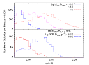
Figure 2.— Top panel: the redshift distribution of the galaxies in our sample with stellar mass: log $M_{\star}/M_{\odot}=10.0\pm 0.05$, $10.5\pm 0.05$, and $11.0\pm 0.05$. Bottom panel: the redshift distributions of the log $M_{\star}/M_{\odot}=10.5$ galaxies, with log SFR [$M_{\odot}$yr^-1] = $0.2\pm 0.05$ and $0.8\pm 0.05$.

To investigate the redshift evolution further, we plot the median metallicities of the galaxies with log $M_{\star}/M_{\odot}=10.5\pm 0.05$ and various SFR as functions of redshift in figure 3. The metallicities of the high SFR galaxies (log SFR [$M_{\odot}$yr^-1] $\gtrsim 0.5$) is lower at higher redshifts, while the metallicities of the low SFR galaxies shows negative or no evolution, confirming the results in figure 1.

In the bottom panel of figure 2, we show redshift distributions of the galaxies with log $M_{\star}/M_{\odot}=10.5$, and log SFR [$M_{\odot}$yr^-1] $=0.2$ & 0.8. The galaxies with different SFR are sampled from different redshifts, as well as in the case of different $M_{\star}$ shown in the top panel. In figure 1, the SFR–$Z$ relations for the whole redshift range ($0.07<z<0.3$) follows the low redshift relation in the low SFR end, while metallicity of the high SFR galaxies follows the high redshift relation, consistently to the difference of the redshift distributions between the low and high SFR galaxies.

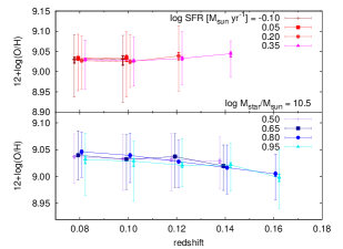
Figure 3.— The metallicity evolution of the galaxies with log $M_{\star}/M_{\odot}=10.5\pm 0.05$. The data points represent the median, the 1$\sigma$ scatter (thin error bars), and the error of mean (thick error bars) of the galaxy metallicities. The width of each bin is 0.02 dex and 0.1 dex for redshift and SFR, respectively. The data points are slightly shifted sideway for visibility.

4. DISCUSSION

4.1. Kolmogorov-Smirnov Test

To examine the significance of the redshift evolution we find in § 3, we perform the two-sample Kolmogorov-Smirnov (KS) test, which calculates the probability that two samples can be drawn from a same probability distribution function. In figure 4, we show metallicity distributions of the galaxies with the four sets of $M_{\star}$ and SFR, which show notable redshift evolution in figure 1, at two different redshifts each.

The positive metallicity evolution (lower-metallicity at higher-redshift) in the mass ranges log $M_{\star}/M_{\odot}\lesssim 10.5$ is statistically significant to high confidence level $>99$% (the top 3 panels of figure 4). The statistical significance of the evolution of the galaxies with log $M_{\star}/M_{\odot}\sim 10.25$ and 10.5 is very high with the KS test probability $P_{\rm KS}=7.7\times 10^{-13}$ and $2.1\times 10^{-7}$.

Although the statistical significance of the evolution of the galaxies with log $M_{\star}/M_{\odot}=10.0$ is lower than in the cases of the galaxies with log $M_{\star}/M_{\odot}\sim 10.25$ and 10.5 due to the very narrow range of redshift where we can investigate log $M_{\star}/M_{\odot}=10.0$ galaxies, the evolution in this mass range is also larger than statistical error ($P_{\rm KS}=1.5\times 10^{-3}$). The extent of the evolution of the galaxies with log $M_{\star}/M_{\odot}=10.0$ is similar to that of the log $M_{\star}/M_{\odot}=10.5$ galaxies ($\sim 0.03$ dex), although the redshift range investigated is 3 times smaller. This suggests that less massive galaxies are more rapidly evolving in metallicity, consistently to the findings of previous studies (e.g., Savaglio et al., 2005, but see also Lamareille et al. 2009).

The possible negative metallicity evolution of the high-mass, low-SFR galaxies is statistically less significant than the positive evolution of the high SFR galaxies (the bottom panel of figure 4), as expected from the large error of mean in figure 1.

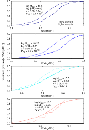
Figure 4.— The cumulative metallicity distributions of the galaxies with the four sets of $M_{\star}$ and SFR, at low and high redshifts. The top 3 panels show the high SFR galaxies whose metallicity is lower at higher redshift, while the bottom panel shows the low SFR galaxies whose metallicity is (possibly) higher at higher redshift. In each panel, solid and dashed histograms represent low and high redshift samples, respectively. The plotted redshifts are different for different set of $M_{\star}$ and SFR, due to the difference of the redshift distributions of the galaxies with different $M_{\star}$ and SFR (see figure 2).

4.2. The Effect of Fiber Covering Fraction

The combination effect of fiber covering fraction and metallicity gradient in a galaxy may cause seeming metallicity evolution with redshift. The SDSS spectroscopic fiber (3 arcsec) contains larger area of a target galaxy at higher redshift, and galaxies tend to have lower metallicity in their outskirt than at their center (e.g., Zaritsky et al., 1994).

We show the relation between the fiber covering fraction (the fiber to total flux ratio in $r$-band) and the derived metallicity of the galaxies with log $M_{\star}/M_{\odot}=10.5$ and log SFR [$M_{\odot}$yr^-1] $=0.8$ in figure 5. The galaxies with larger covering fraction have higher-metallicity, contrary to what is expected from the metallicity gradient. This trend may be a result of the negative correlation between galaxy radius and metallicity found by Ellison et al. (2008). The absence of the expected negative correlation between the fiber covering fraction and the metallicity suggests that the fiber covering fraction is determined by intrinsic size of galaxies rather than their redshift. We note that the galaxies have significant variation of radus (6–15 kpc, Petrosian) even in the narrow bin of $M_{\star}$ and SFR.

It should be noted that the gradient effect may be hidden in figure 5 canceled by the effect of the radius–metallicity correlation, and hence the absence of the gradient effect in the plot doesn’t completely rule out the effect. However, if the redshift evolution of metallicity results from the effect of the metallicity gradient, we expect larger evolution for galaxies with larger radius and the gradient. Considering that galaxies with larger $M_{\star}$ tend to have larger radius, and dwarf galaxies have flatter metallicity gradient than spirals (e.g., Lee et al., 2006), the finding of the metallicity evolution only in high specific SFR galaxies is opposite to the expected trend in the case of the gradient effect. Hence we consider it is difficult to explain the metallicity evolution found in this study only by the effect of the metallicity gradient.

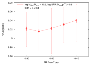
Figure 5.— The median, the 1$\sigma$ scatter, and the error of mean of the galaxy metallicities with log $M_{\star}/M_{\odot}=10.5$ and log SFR [$M_{\odot}$yr^-1] $=0.8$, as a function of the fiber covering fraction. Here the fiber covering fraction is the ratio of flux in fiber to total flux of the object measured in $r$-band. The width of the fiber covering fraction bins is 0.1 dex.

4.3. Continuum and H$\alpha$ Line Luminosity Limits

As mentioned in § 2, the SDSS spectroscopic target galaxies are magnitude limited $m_{r,{\rm Pet}}\leq 17.77$, and we select galaxies with H$\alpha$ S/N $>25$ for this study. Hence the broad band limiting magnitude and/or the H$\alpha$ flux limit may cause some redshift dependent sampling bias.

In figure 6, we plot $M_{r}$ and H$\alpha$ luminosity distributions of the galaxies with log $M_{\star}/M_{\odot}=10.5$ and log SFR [$M_{\odot}$yr^-1] $=0.8$ at redshift 0.08 and 0.14. With the fixed $M_{\star}$ and SFR, the galaxies at $z=0.14$ are clearly brighter than the $z=0.08$ galaxies in $r$-band, suggesting that the $r$-band limiting magnitude plays an important role in this sample. On the other hand, the H$\alpha$ luminosity distributions at the two different redshifts are not largely different. We note that galaxies with log SFR [$M_{\odot}$yr^-1] $=0.8$ typically have H$\alpha$ S/N $\sim 60$ at $z=0.14$, and hence few galaxies in this SFR range are rejected by the H$\alpha$ S/N limit by the H$\alpha$ S/N threshold.

To discuss the effect of the limiting magnitude, we plot distributions of the galaxies with log $M_{\star}/M_{\odot}=10.5$ in some redshift bins on the SFR versus $r$-band mass-to-luminosity ratio ($M_{\star}/L_{\nu,r}$) plane and the metallicity versus $M_{\star}/L_{\nu,r}$ plane in figure 7.

In the left panel of figure 7, $M_{\star}/L_{\nu,r}$ of the galaxies clearly correlates with SFR, causing the difference of redshift distribution between the galaxy samples with different SFR (the bottom panel of figure 2). On the other hand, no clear correlation between metallicity and $M_{\star}/L_{\nu,r}$ is seen in the right panel. Furthermore, it is also notable that galaxies at higher redshifts have systematically lower metallicity than lower redshift galaxies with similar $M_{\star}/L_{\nu,r}$.

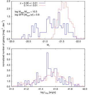
Figure 6.— Top panel: the $r$-band luminosity distribution of the galaxies with log $M_{\star}/M_{\odot}=10.5$ and log SFR [$M_{\odot}$yr^-1] $=0.8$ sampled from the two different redshifts. Bottom panel: same as the top panel, but the H$\alpha$ luminosity distribution.

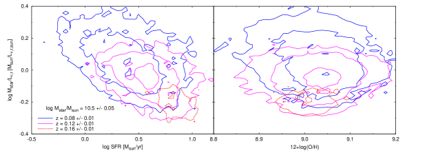
Figure 7.— Left panel: the distribution of the galaxies with log $M_{\star}/M_{\odot}=10.5$, on the SFR versus mass-to-luminosity ratio plane. The distributions of the galaxies at $z=0.08,0.12$ and $0.16\pm 0.01$ are shown with solid (blue), dashed (magenta), and dotted (red) contours, respectively. The contours indicates $d^{2}n_{\rm gal}/d{\rm logSFR}d{\rm log}(M_{\star}/L_{\nu,r})=1,3,9\ldots$ [dex^-2]. The $r$-band solar luminosity is $L_{\nu,r,\odot}=5.9\times 10^{18}$ erg sec^-1 Hz^-1 (Blanton et al., 2003). Right panel: same as the left panel, but on the metallicity versus mass-to-luminosity ratio plane.

To test the effect of the limiting magnitude further, we separate the galaxies with log $M_{\star}/M_{\odot}=10.5$ and log SFR [$M_{\odot}$yr^-1] $=0.8$ at redshift 0.08 into two subsamples. One is bright ($M_{r}<-21.5$), and the other is faint ($M_{r}\geq 21.5$). We compare the metallicity distributions of the bright/faint samples at $z=0.08$ and the sample at $z=0.14$ in figure 8. The galaxies in the bright sample at $z=0.08$ have similar $M_{r}$ to the galaxies at $z=0.14$. Although the bright sample is small, the KS test between the bright sample and the $z=0.14$ sample indicates the metallicity distributions of the two sample is significantly different ($P_{\rm KS}=0.037$), while the faint sample and the bright sample is broadly consistent ($P_{\rm KS}=0.31$). Hence it is unlikely that the limiting magnitude effect is the primary source of the redshift evolution of the $M_{\star}$–SFR–$Z$ relation.

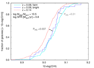
Figure 8.— The cumulative metallicity distributions of the galaxies with log $M_{\star}/M_{\odot}=10.5$ and log SFR [$M_{\odot}$yr^-1] $=0.8$, at the two different redshifts. The low redshift sample is separated into the bright ($M_{r}<-21.5$) and the faint ($M_{r}\geq 21.5$) subsamples. The galaxies in the bright sample have similar $M_{r}$ to that of the high redshift sample, where faint galaxies are not selected as spectroscopic targets. The KS test probabilities between the distributions are indicated together.

4.4. Noise Effect and Mean Spectra

With similar $M_{\star}$ and SFR, spectra of high redshift galaxies would have lower S/N than those of low redshift galaxies. This expected trend possibly affect the metallicity estimate in a redshift dependent way. We also note that figure 6 suggests that high redshift galaxies have smaller H$\alpha$ equivalent width than low redshift galaxies, and hence it is possible that high redshift galaxies suffer more from uncertainties of the continuum subtraction than low redshift galaxies. To reduce the noise effect, we compose mean spectra of the galaxies with log $M_{\star}/M_{\odot}=10.5\pm 0.05$ and log SFR [$M_{\odot}$yr^-1] $=0.8\pm 0.05$ at redshifts $0.08\pm 0.01,\ 0.10\pm 0.01,\ 0.12\pm 0.01,\ 0.14\pm 0.01$, and $0.16\pm 0.01$, and measure [NII]$\lambda$6584/H$\alpha$ and $R_{23}$ of the mean spectrum at each redshift.

We average spectra collected from the SDSS data archive server after shifting wavelength to the center of each redshift bin. To reduce the effect of stellar absorption lines on the emission line measurement, we fit continuum of the mean spectra with stellar spectral energy distribution (SED) models, and subtract the stellar component models form the mean spectra. We perform the SED fitting with the SEDfit software package (Sawicki, 2012; Sawicki & Yee, 1998) which utilize the population synthesis models of Bruzual & Charlot (2003). We examine five cases of star formation history: simple stellar population, constant star formation, and exponentially decaying star formation with $\tau=$ 0.2, 1.0, and 5.0 Gyr assuming stellar metallicity to be $Z_{\odot}$.

Two mean spectra and their best fit stellar SED models are shown in the left panel of figure 9. The mean spectra achieves very high S/N (typically $\sim$ 100 in the highest redshift bin). The best fit parameters of the stellar SED models indicate smaller $M_{\star}$ and SFR than log $M_{\star}/M_{\odot}=10.5$ and log SFR [$M_{\odot}$yr^-1] $=0.8$, but we note that the spectra only represents stellar populations in the spectroscopic fiber. In the right panel of figure 9, we show a close up view of high order Balmer lines in the mean spectra. Although the center of each absorption line is affected by the corresponding emission line, the stellar SED models reproduce Balmer absorption lines in their wings.

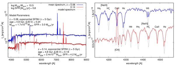
Figure 9.— Left panel: the mean spectra of the galaxies with log $M_{\star}/M_{\odot}=10.5$ and log SFR [$M_{\odot}$yr^-1] $=0.8$, at $z=$ 0.08 and 0.14. The model stellar spectra are plotted together with the model parameters indicated. Right panel: a close up view of high order Balmer lines in the mean spectra shown in the left panel.

After subtracting the stellar SED models, we fit each line with linear continuum plus single gaussian to measure flux of each line (we fit [OII]$\lambda$3727 doublet with linear continuum plus double gaussian). We show the line fittings at $z=$ 0.08 and 0.14 in figure 10 and 11. When normalized to the peaks of the gaussian models of H$\alpha$, the spectrum at $z=0.08$ has slightly stronger [NII]$\lambda$6584 than the spectrum at $z=0.14$ (figure 10). We also fit [NII]$\lambda$6548 to avoid that the line affects the estimate of the residual continuum, although we don’t use the line as a metallicity indicator. One can also find that [OII]$\lambda$3727 is slightly weaker at $z=0.08$ than at $z=0.14$ (figure 11), contrary to the case of [NII]$\lambda$6584. We note that the continuum level underneath [OII]$\lambda$3727 may be affected by high order Balmer emission lines whose peaks are not resolved in the mean spectra, and it may affect $R_{23}$, while [NII]/H$\alpha$ is free from this effect.

The line fluxes obtained by the gaussian fit are listed in table 1 after corrected for extinction using H$\alpha$/H$\beta$ ratio and the Cardelli et al. (1989) extinction curve. The redshift evolution of the metal indicating line ratios is plotted in figure 12, together with the median line ratios of the galaxies with the same $M_{\star}$, SFR, and redshift to those of the mean spectra. Note that the line fluxes of the mean spectra are obtained by our gaussian fit, while the median line ratios are obtained using the line fluxes listed in the MPA-JHU catalog.

Galaxies at higher redshifts show smaller [NII]/H$\alpha$ and larger $R_{23}$, in their mean spectra. The relations between the line ratios and $Z$ are $d{\rm log([NII]/H\alpha)}/d{\rm log}Z=0.81$ and $d{\rm log}R_{23}/d{\rm log}Z=-1.5$ at 12 + log(O/H) = 9.0 (Maiolino et al., 2008), and hence the evolution of the line ratios in figure 12 is broadly consistent to the metallicity evolution found in § 3. The median line ratios also evolve with similar manner to the line ratios of the mean spectra, although they indicate smaller metal-to-hydrogen line ratio than the results with the mean spectrum, possibly due to the difference of spectrum fitting method. Thus we conclude that the metallicity evolution is not a result of noise effect.

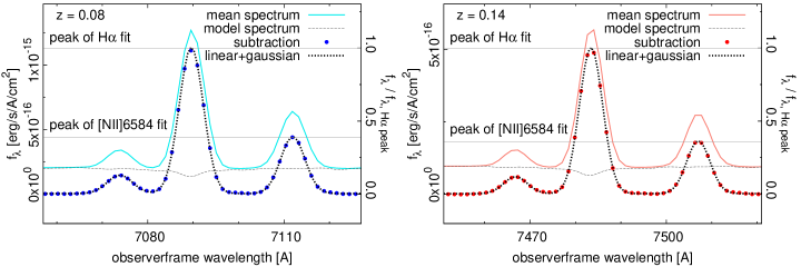
Figure 10.— [NII] and H$\alpha$ lines in the mean spectra at $z=$ 0.08 and 0.14. Solid and dashed curves are the mean spectra and the model spectra which are shown in figure 9. The model subtracted spectra are plotted as data points (filled circle), to which we perform the linear continuum plus gaussian fitting. Note that the noise level is too small to plot. The results of the line fittings are shown with dotted lines. The peaks of the gaussian models of H$\alpha$ and [NII]$\lambda$6584 lines are indicated with horizontal lines. The right vertical axis in each panel indicates $f_{\lambda}$ normalized to the peak of the gaussian fit of H$\alpha$ line.

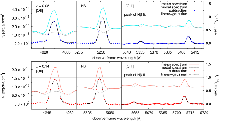
Figure 11.— Same as figure 10, but for $R_{23}$ lines. The right vertical axis indicates $f_{\lambda}$ normalized to the peak of H$\beta$ line.

Table 1The Emission Lines in the Mean Spectra

redshift	[OII]$\lambda$3727	H$\beta$	[OIII]$\lambda$4959	[OIII]$\lambda$5007	H$\alpha$	[NII]$\lambda$6584
0.08	$2.72\times 10^{-14}$	$1.50\times 10^{-14}$	$1.50\times 10^{-15}$	$4.15\times 10^{-15}$	$3.86\times 10^{-14}$	$1.51\times 10^{-14}$
0.10	$1.91\times 10^{-14}$	$9.98\times 10^{-15}$	$9.95\times 10^{-16}$	$2.88\times 10^{-15}$	$2.57\times 10^{-14}$	$9.80\times 10^{-15}$
0.12	$1.34\times 10^{-14}$	$6.86\times 10^{-15}$	$7.32\times 10^{-16}$	$2.10\times 10^{-15}$	$1.78\times 10^{-14}$	$6.40\times 10^{-15}$
0.14	$9.18\times 10^{-15}$	$4.76\times 10^{-15}$	$5.38\times 10^{-16}$	$1.46\times 10^{-15}$	$1.24\times 10^{-14}$	$4.46\times 10^{-15}$
0.16	$8.14\times 10^{-15}$	$3.58\times 10^{-15}$	$4.37\times 10^{-16}$	$1.27\times 10^{-15}$	$9.36\times 10^{-15}$	$3.31\times 10^{-15}$

Note. — The extinction corrected line fluxes of the mean spectra of the galaxies with log $M_{\star}/M_{\odot}=10.5\pm 0.05$ and log SFR [$M_{\odot}$yr^-1] $=0.8\pm 0.05$. The units are [erg s^-1 cm^-2].

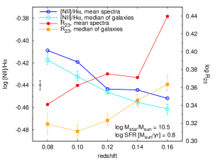
Figure 12.— The redshift evolution of the metal indicating line ratios of the mean spectra. The median line ratios of the galaxies with the same $M_{\star}$, SFR, and redshift are plotted together. Each line is detected with S/N = 100–1000 in the mean spectra, where the vertical error bar in the left corresponds to S/N = 100. The vertical error bars of the median line ratios indicate the error of mean.

5. SUMMARY

We have investigated the evolution of the $M_{\star}$–SFR–$Z$ relation at $z<0.3$. Although the redshift range we investigated is narrow, we found metallicity of the high SFR galaxies (log SFR [$M_{\odot}$yr^-1] $\gtrsim 0.5$) with log $M_{\star}/M_{\odot}\lesssim 10.5$ is evolving with $>99$% statistical significance. We have examined the observational effects which may cause seeming evolution of metallicity: the fiber aperture effect, the sampling bias by the limiting magnitude, and the noise in the spectra. We found it is difficult to explain the evolution of the $M_{\star}$–SFR–$Z$ relation only by the observational effects, although some effects are not completely ruled out.

In the current galaxy sample at low redshifts, galaxies with different $M_{\star}$ and SFR are sampled with different redshift distributions, and there is a degeneracy between $M_{\star}$/SFR, and redshift. Hence it is difficult to clearly separate SFR dependence of metallicity from redshift dependence. The metallicity evolution of galaxies with same $M_{\star}$ and SFR at $z<0.3$ found in this study suggests that the currently known $M_{\star}$–SFR–$Z$ relation arises from a combination of the intrinsic relation and the redshift evolution effect. Previous studies (e.g., M10; Lara-López et al., 2010) showed that $z>0.5$ galaxies agree with the extrapolation of the relation defined by $z<0.3$ galaxies, suggesting that the relation is not evolving with redshift. However, if the redshift evolution effect is included in the relation at $z<0.3$, the agreements of high redshift galaxies don’t necessarily mean that the relation is not evolving. The agreements may result from the extrapolation of the redshift evolution effect.

We need to investigate metallicity distribution of galaxies with same $M_{\star}$ and SFR at different redshifts, to distinguish the intrinsic relation from the redshift evolution effect. However, it is currently possible only for narrow range of $M_{\star}$, SFR, and redshift. The extent of the evolution we find in the current sample is very small due to the very narrow range of redshift we can investigate. Hence it is difficult to robustly exclude possibility of systematic effects in our results.

Deeper wide field spectroscopic survey which covers wider range of redshift is necessary to test the evolution effect more robustly. For example, to study similar range of $M_{\star}$ and SFR at $z\sim 1$ with a comparable sample number (or a survey volume, $\gtrsim$ 10%) to this study, the limiting magnitude must be 5 magnitude deeper than the SDSS sample ($m\lesssim 23$), and the survey field must be $\gtrsim$ 20 deg² (0.3% of the SDSS DR7 field). Note that the comoving volume element is $\sim$ 37 times larger at $z=1$ than at $z=0.1$. Future spectroscopic surveys, such as Subaru Measurement of Images and Redshifts (SuMIRe) project, will achieve such requirements. At redshifts $z<1$, the limiting magnitude can be brighter but the survey field must be wider. The robust separation of the intrinsic $M_{\star}$–SFR–$Z$ relation from its evolution will open a new way to understand galaxy evolution.

References

- Blanton et al. (2003) Blanton, M. R., et al. 2003, ApJ, 592, 819
- Brinchmann et al. (2004) Brinchmann, J., Charlot, S., White, S. D. M., Tremonti, C., Kauffmann, G., Heckman, T., & Brinkmann, J. 2004, MNRAS, 351, 1151
- Brisbin & Harwit (2012) Brisbin, D., & Harwit, M. 2012, ApJ, 750, 142
- Bruzual & Charlot (2003) Bruzual, G., & Charlot, S. 2003, MNRAS, 344, 1000
- Cardelli et al. (1989) Cardelli, J. A., Clayton, G. C., & Mathis, J. S. 1989, ApJ, 345, 245
- Cresci et al. (2012) Cresci, G., Mannucci, F., Sommariva, V., Maiolino, R., Marconi, A., & Brusa, M. 2012, MNRAS, 421, 262
- Davé et al. (2012) Davé, R., Finlator, K., & Oppenheimer, B. D. 2012, MNRAS, 421, 98
- Dayal et al. (2012) Dayal, P., Ferrara, A., & Dunlop, J. S. 2012, arXiv:1202.4770
- Eisenstein et al. (2001) Eisenstein, D. J., et al. 2001, AJ, 122, 2267
- Ellison et al. (2008) Ellison, S. L., Patton, D. R., Simard, L., & McConnachie, A. W. 2008, ApJ, 672, L107
- Erb et al. (2006) Erb, D. K., Shapley, A. E., Pettini, M., Steidel, C. C., Reddy, N. A., & Adelberger, K. L. 2006, ApJ, 644, 813
- Kauffmann et al. (2003a) Kauffmann, G., et al. 2003a, MNRAS, 341, 33
- Kauffmann et al. (2003b) —. 2003b, MNRAS, 346, 1055
- Lamareille et al. (2009) Lamareille, F., et al. 2009, A&A, 495, 53
- Lara-López et al. (2010) Lara-López, M. A., et al. 2010, A&A, 521, L53
- Lee et al. (2006) Lee, H., Skillman, E. D., & Venn, K. A. 2006, ApJ, 642, 813
- Liu et al. (2008) Liu, X., Shapley, A. E., Coil, A. L., Brinchmann, J., & Ma, C.-P. 2008, ApJ, 678, 758
- Maiolino et al. (2008) Maiolino, R., et al. 2008, A&A, 488, 463
- Mannucci et al. (2010) Mannucci, F., Cresci, G., Maiolino, R., Marconi, A., & Gnerucci, A. 2010, MNRAS, 408, 2115
- Nakajima et al. (2012) Nakajima, K., et al. 2012, ApJ, 745, 12
- Richard et al. (2011) Richard, J., Jones, T., Ellis, R., Stark, D. P., Livermore, R., & Swinbank, M. 2011, MNRAS, 413, 643
- Salim et al. (2007) Salim, S., et al. 2007, ApJS, 173, 267
- Savaglio et al. (2005) Savaglio, S., et al. 2005, ApJ, 635, 260
- Sawicki (2012) Sawicki, M. 2012, accepted for publication in PASP (arXiv:1210.0285)
- Sawicki & Yee (1998) Sawicki, M., & Yee, H. K. C. 1998, AJ, 115, 1329
- Stoughton et al. (2002) Stoughton, C., et al. 2002, AJ, 123, 485
- Strauss et al. (2002) Strauss, M. A., et al. 2002, AJ, 124, 1810
- Tremonti et al. (2004) Tremonti, C. A., et al. 2004, ApJ, 613, 898
- Wuyts et al. (2012) Wuyts, E., Rigby, J. R., Sharon, K., & Gladders, M. D. 2012, arXiv:1202.5267
- Yabe et al. (2011) Yabe, K., et al. 2011, arXiv:1112.3704
- Yates et al. (2012) Yates, R. M., Kauffmann, G., & Guo, Q. 2012, MNRAS, 422, 215
- Zaritsky et al. (1994) Zaritsky, D., Kennicutt, Jr., R. C., & Huchra, J. P. 1994, ApJ, 420, 87