Spatial Coherence of a polariton condensate in 1D acoustic lattice

Abstract

Several mechanisms are discussed which could determine the spatial coherence of a polariton condensate confined to a one dimensional wire. The mechanisms considered are polariton-polariton interactions, disorder scattering and non-equilibrium occupation of finite momentum modes. For each case, the shape of the resulting spatial coherence function $g^{(1)}\left(x\right)$ is analysed. The results are compared with the experimental data on a polariton condensate in an acoustic lattice from [E. A. Cerda-Mendez et al, Phys. Rev. Lett. 105, 116402 (2010)]. It is concluded that the shape of $g^{(1)}\left(x\right)$ can only be explained by non-equilibrium effects, and that $\sim 10$ modes are occupied in the experimental system.

I Introduction

The fabrication of planar (2D) microcavities has provided experimental access to the strong coupling regime between light and matter in a spatially extended system Weisbuch . The excitations of the coupled modes are polaritons, quasi-particles which are bosons with a very small effective mass, typically $10^{-4}$ times that of an electron. This makes it possible to study quantum effects in a solid state system at a relatively high temperatures SkolnickFischerWhittaker . The short life time of the polaritons, $\sim 5$ ps Balili , means that the system has to be constantly pumped to observe Bose-Einstein condensation (BEC). It can be achieved either resonantly Stevenson or non-resonantly Kasprzak producing condensates with long coherence times Love and long range spatial coherence Balili ; Kasprzak ; Wertz . These have been shown to exhibit interesting nonlinear and many-body phenomena, such as vortex formation Lagoudakis08 ; Krizhanovskiivortex , solitons AmoSoliton and superfluid-like flow AmoSuperfluid .

In recent experiments Wertz ; Krizhanovskii , microcavity polaritons have been confined in wire like geometries, to study the peculiar interaction effects of bosons in a 1D system as well as a step to the realisation of polariton circuits Liew . The extra confinement was provided in two different ways: by etching of the whole planar structure to form a wire Wertz and by excitation of surface acoustic waves (SAW) to form a dynamic 1D lattice Krizhanovskii . It is the spatial coherence measurements in the latter setup that are the subject of the present paper. In the experiment, the same sample area was studied with and without the SAW, so it was possible to measure how the coherence length changed when the 1D confinement was introduced. Without confinement, the entire 2D emission spot was coherent, that is, the coherence length was the same as the spot size Krizhanovskii ; Deng2007 . With confinement it was observed that the coherence length in the direction perpendicular to the SAW wavefronts was reduced to the SAW wavelength, as the condensates confined in the individual minima became decoupled. However, there was also a significant reduction in the coherence length measured parallel to the wavefronts Krizhanovskii , along the ‘wires’, which is less easily explained.

In this paper we analyse possible mechanisms for the reduction of the spatial coherence along the 1D wires. We consider the effect polariton_phonon of polariton-polariton interactions, disorder, and finite momentum modes occupation in a harmonic trap on the first order correlation function $g^{(1)}\left(x\right)$. The theoretical predictions are compared with the experimentally measured $g^{(1)}\left(x\right)$ exp_data which has a Gaussian shape up to the noise floor. This shape can only be reproduced by the non-equilibrium occupation of a set of the finite momentum modes. Performing a more quantitative fit, using the occupation numbers as fitting parameters, we find that the number of the excited modes in the experiment Krizhanovskii is $\sim 10$.

The rest of the paper is organised as follows. In Section 2 we formulate the model of the 1D polariton system with different types of interactions. In Section 3 we calculate the spatial dependence of the coherence function $g^{(1)}\left(x\right)$ when finite momentum modes are occupied in a harmonic trap. Section 4 contains discussion of the Anderson localisation due to disorder in a 1D system. In Section 5 we discuss the effect of the short range polariton-polarion interaction on $g^{(1)}\left(x\right)$. Section 6 contains the fitting of the experimental data with the theoretical predictions from the previous sections.

II Model

We consider one dimensional polaritons formed by the equal mixture of exciton and photon at the zero momentum following the experimental setup of Krizhanovskii .

The motion of photons in $z-$direction is restricted by a planar microcavity which is formed by a pair of Bragg mirrors giving a small mass to the 2D photons $C_{\mathbf{k}}$. Excitons are bound electron-hole pairs, they are bosons $X_{\mathbf{k}}$, which are confined to the same 2D plane by a quantum well, see the scheme in Fig. 1. The eigenmodes of a strongly interacting $X_{\mathbf{k}}$ and $C_{\mathbf{k}}$ are two hybrid particles, Lower and Upper polarions (LP and UP). We will consider only the LP branch as bosons $a_{\mathbf{k}}$ with a parabolic dispersion and mass $m_{LP}$ assuming that the photons and the excitons are at resonance at $\mathbf{k}=0$, e. g. a LP around the zero momentum consists of equal mixture of the exciton and the photon $a_{\mathbf{k}}=\left(X_{\mathbf{k}}+C_{\mathbf{k}}\right)/\sqrt{2}$.

Bosonic nature of these polaritons allows a macroscopic occupation of the single zero momentum state that leads to a long-range phase coherence in the system. Access to this regime is not straightforward as the short lived polaritons do not have time to relax at low momenta due to a slow emission of the low energy phonons forming a relaxation bottleneck and forbidding formation of the truly equilibrium condensate. This difficulty can be overcome in a nonequilibrium regime under a strong pumping when the $\mathbf{k}=0$ state is populated directly or indirectly by employing an optical parametric oscillator (OPO).

In the OPO scheme the system is excited by the pump at a finite momentum $\mathbf{k}_{p}$ and energy $E_{p}$. Due to the polariton-polariton interactions the $\mathbf{k}_{p}$ excitations can scatter fast to a low momentum. Above a threshold density of the directly pumped polaritons the interaction becomes strong enough to reach the zero momentum state $\mathbf{k}_{s}=0$, signal, which also forms a significant population in the idler state $\mathbf{k}_{i}$ due to the conservation of the energy $E_{i}+E_{s}=E_{p}$ and the momentum $\mathbf{k}_{i}+\mathbf{k}_{s}=\mathbf{k}_{p}$ by the scattering process. Above the threshold the systems locks only to these three states Stevenson with a significant population of the signal state at $\mathbf{k}_{s}=0$. This approach is more advantageous than the direct pumping as in the OPO regime the pump at a finite $\mathbf{k}_{p}$ does not obstruct the emission from the condensate at $\mathbf{k}_{s}=0$.

The 2D polaritons are constrained further to a set of 1D wires by an in-plane surface acoustic wave propagating along $y$-direction, see the scheme in Fig. 1. The $y$-component of the momentum belongs to the lowest energy subband leaving the only motion along $x$-axis unconstrained. The polaritons are detected though the photonic part which constantly escapes the system forming a spatial distribution of the electric field outside of the cavity that contains information about the polaritons inside the structure,

$$E\left(x\right)=\sum_{k}\sqrt{\frac{\epsilon_{k}}{L}}\left(\varphi_{k}^{*}\left(x\right)C_{k}^{\dagger}-\varphi_{k}\left(x\right)C_{k}\right),$$ (1)

and can be registered by a detector. Here $\varphi_{k}\left(x\right)$ are the eigenmodes of the external potential in $x$-direction, e. g. $\varphi_{k}\left(x\right)=e^{ikx}$ if the there is no extra potential along $x$-axis, $\epsilon_{k}$ is the dispersion of the electro-magnetic modes, and $L$ is the length of the wire.

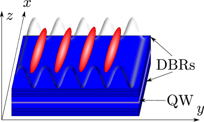
Figure 1: Scheme of the microcavity (DBRs) with a quantum well inside (QW), and the surface acoustic wave (red elongated ellipses are the polariton 1D wires).

We consider three possible mechanisms that can affect spatial coherence of free polaritons in the signal, $a_{k}^{\dagger}$ around $k_{s}=0$. First is a confining potential originating from a finite size of the excitation spot. We assume that the single particle potential is harmonic,

$$U_{\textrm{harmonic}}=\frac{m_{LP}\omega^{2}x^{2}}{2},$$ (2)

where the frequency $\omega$ defines the system size as $L=\sqrt{2\hbar/\left(m_{LP}\omega\right)}$. Second is a disorder potential that has a finite correlation length $l_{0}$,

$$\overline{U_{\textrm{disorder}}\left(x\right)U_{\textrm{disorder}}\left(x^{\prime}\right)}=F\left(\frac{x-x^{\prime}}{l_{0}}\right)$$ (3)

where $F\left(y\right)$ is a function that vanished when $\left|x-x^{\prime}\right|\gg l$, i. e. $F\left(0\right)=U_{0}$ and $F\left(y\gg 1\right)=0$. And the third mechanism is the pair polariton-polariton interaction. It has a short range interaction potential as the polaritons have zero electric charge with the interaction strength $V_{0}$.

We neglect the interaction of polariton with phonons mechanism for decoherence as it is ineffective at low momenta. The polariton-phonon scattering time is $\sim 100$ ps Tassone which is much longer than the polariton life time $\sim 5$ ps. The latter is due to detuning chosen in the experiment Krizhanovskii where the polaritons at $\mathbf{k}\approx 0$ consist of the equal mixture of the exciton and the photon.

To analyse the spatial coherence that is observed via the photonic part of the LP we consider the first order correlation function,

$$g^{(1)}\left(x\right)=\frac{\left\langle\hat{N}\left[E^{\dagger}\left(x\right)E\left(-x\right)\right]\right\rangle}{\left\langle\hat{N}\left[E^{\dagger}\left(0\right)E\left(0\right)\right]\right\rangle},$$ (4)

where $\hat{N}\left[\dots\right]$ is the normal ordering operator that eliminates the vacuum fluctuations of the quantised electro-magnetic field and $\left\langle\dots\right\rangle$ is the average with respect to a state of the system.

The eigenstates of the free polariton Hamiltonian are plain waves. The expectation value over the zero momentum state occupied by many polaritons gives an infinite range coherence, $g^{(1)}\left(x\right)=1$. In the next three sections we analyse each of the possible mechanisms separately to see how they restrict this behaviour.

III Finite momentum modes in a trap

Here we obtain the single particle eigenstates of polaritons in the harmonic trap. Then we evaluate $g^{(1)}\left(x\right)$ as the expectation value with respect to a density matrix assuming a non-equilibrium distribution of the polariton occupation numbers around the zero momentum state.

The single particle Hamiltonian for a polariton in a harmonic potential,

$$H=\frac{p^{2}}{2m_{LP}}+U_{\textrm{harmonic}},$$ (5)

is the one of the quantum harmonic oscillator. It is a well known and solved model.

Following the standard approach to the diagonalisation problem we search for a solution in form of a polynomial Schiff . The eigenfunction problem for the model Eq. (5) leads to Hermite’s differential equation which is solved by

$$\psi_{k}\left(x\right)=\frac{1}{\sqrt{2^{k}k!}}\left(\frac{2}{\pi}\right)^{\frac{1}{4}}\frac{1}{\sqrt{L}}e^{-x^{2}/L^{2}}H_{k}\left(\frac{\sqrt{2}x}{L}\right),$$ (6)

where $H_{k}\left(z\right)=\left(-1\right)^{k}e^{z^{2}}d^{k}e^{-z^{2}}/dz^{k}$ are the Hermite polynomials, $L=\sqrt{2\hbar/\left(m_{LP}\omega\right)}$ is the size of the system, and $k$ is the number of the energy level that describes a finite momentum state of the 1D polariton. The complementary eigenvalue problem can be solved via a Taylor expansion. As a result the eigenenergies of the finite momentum states $k\neq 0$ have a linear spectrum

$$E_{k}=\omega\left(k+\frac{1}{2}\right).$$ (7)

A many polariton state, which is created in a pumping process, is described by a density matrix. The expectation value in the correlation function Eq. (4) has to be evaluated as an ensemble average,

$$\left\langle\dots\right\rangle=\textrm{Tr}\hat{\rho}\dots,$$ (8)

where $\hat{\rho}$ is a density matrix.

In a continuous wave experiment the signal is accumulated on the time scale of seconds. The phase coherence of a polariton condensate is limited by few hundreds of pico-seconds Love which partitions the long accumulation interval into a large ensemble of many very short measurements. Thus the total signal is averaged over many realisations with different distribution of the polariton occupation numbers and the total number of polaritons which also changes slightly in time due to the power fluctuation in the pumping laser Love . As the phase coherence is lost between different realisations the density matrix, which describes such an ensemble, is diagonal in the representation of the polariton occupation numbers,

$$\hat{\rho}=\sum_{n_{0}n_{1}\dots}\rho_{n_{0}n_{1}\dots}\left|n_{0}n_{1}\dots\left\rangle\right\langle n_{0}n_{1}\dots\right|$$ (9)

Here $\left|n_{0}n_{1}\dots\right\rangle$ is a state with $n_{0}$ polaritons at the momentum $k=0$, $n_{1}$ polaritons at the momentum $k=1$, etc and $\rho_{n_{0}n_{1}\dots}$ are the diagonal matrix elements that describe a non-equilibrium distribution of the boson occupation numbers.

Substituting Eqs. (8) in Eq. (4) and using the eigenfunction Eq. (6) we obtain the first order coherence function as sum over a set of finite momentum modes,

$$g^{(1)}\left(x\right)=\sum_{k=0}^{\infty}\psi_{k}\left(x\right)\psi_{k}\left(-x\right)p_{k},$$ (10)

where $p_{k}=\sum_{n_{0}n_{1}\dots}n_{k}\rho_{n_{0}n_{1}\dots}/\sum_{n_{0}n_{1}\dots}\rho_{n_{0}n_{1}\dots}$ are weight factors, e. g. in thermal equilibrium they are given by the Bose-Einstein distribution function. Note that $p_{k}$ are not completely equivalent to the occupation number of the polaritons, $n_{k}$, due to the normalisation of the correlation function in Eq. (4).

When only a few low momenta modes are excited with probabilities that are approximately equal, $p_{k}\simeq p_{l}$, the shape of the correlation function is almost Gaussian with a reduced system size $\tilde{L}<L$, $g^{(1)}\left(x\right)\simeq e^{-x^{2}/\tilde{L}^{2}}$. When many modes are excited with an arbitrary $p_{k}$ the shape is arbitrary as polynomials in Eq. (6) of a high order $k\gg 1$ can approximate a wide range of different functions.

IV Anderson Localisation

Polaritons are subject to a random potential which originates from two sources. One is disorder of the quantum well that influences the exciton component of polaritons. And another is imperfections of the cavity mirrors that influences the photon component Kavokin2003 ; Keeling2004 . Here we consider a simplified model of the disorder characterised by a single correlation length Eq. (3) and we assume that the wave length of the surface acoustic wave is smaller then the correlation length of disorder potential in the 2D heterostructure to model the strictly 1D system. If the latter is not true the polariton wire becomes a quasi-1D system which would give a longer localisation length. In this section we also neglect interplay between disorder and polariton-polariton interactions which can lead to a many body metal-insulator transition above a finite temperature Paul ; Aleiner and consider the low temperature case only.

Scaling analysis of the potential disorder problem scaling shows that conductance of a 1D system is zero at low temperatures as all of the zero momentum states become localised when the system size increases to infinity. The lowest energy eigenstates of the single particle model,

$$H=\frac{p^{2}}{2m_{LP}}+U_{\textrm{disorder}},$$ (11)

are localised with the exponential tails $\left|\psi\left(x\right)\right|\sim e^{\left(-\left|x\right|/\xi\right)}$, for example see a review EversMirlin . Therefore the first order correlation function in Eq. (4) evaluated with respect to these states gives a finite coherence length with the same exponential tail,

$$g^{(1)}\left(x\right)\sim e^{-|x|/\xi},$$ (12)

where, in general, the localisation length $\xi$ is not equal to the correlation length of the random potential $l_{0}$.

Here we do not perform a more detailed study of the features that are specific to the disorder in the polariton systems, e.g. Malpuech , but only use the exponential tails of the correlation function as a characteristic feature of the localisation mechanism.

V Polariton-Polariton interactions

The Mermin-Wagner theorem MerminWagner states that a long range order in a 1D system is absent due to any finite-range exchange interaction which results in a large long-range quantum fluctuations. In this section we discuss the manifestation of this general statement in the specific system of interacting 1D polaritons.

The exciton component of a polariton has zero charge but a finite dipole moment. Neglecting the photonic non-linearity, interaction between two polaritons has dipole-dipole nature thus it is short range. This interaction limits temporal coherence of the polariton condensate Love . The spatial coherence, within the model of density-density interaction with the delta-function interaction, was was analysed in details in CarusottoCuiti ; WoutersCarusotto .

It was shown that the coherence length is finite which is manifested by the exponential tails of the coherence function,

$$g^{(1)}\left(x\right)\sim e^{-x/l_{c}},$$ (13)

in accordance with the general Mermin-Wagner theorem MerminWagner that forbids an infinite range order in the 1D systems. It was also shown in WoutersCarusotto that the coherence length decreases with increase of the interaction constant, $l_{c}\sim 1/V_{0}$. For a typical GaAlAs microcavity the estimate of $l_{c}$ was given as few hundred micrometers in an optimal regime.

Note that the functional form of the coherence function due to the polariton interactions Eq. (13) and due to disorder Eq. (12) coincides in the tails.

VI Fitting of experimental data

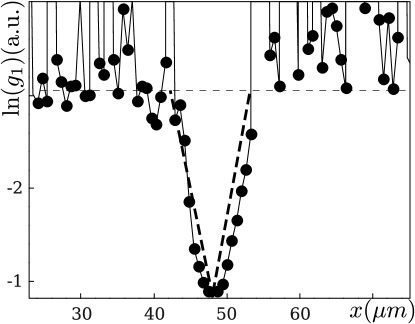
Figure 2: Coherence function $g^{(1)}$ measured along 1D wire on the logarithmic scale. The thin dashed line marks the noise floor and the thick dashed line is an exponential function.

Figure 3: Coherence function $g^{(1)}$ measured along 1D wire on the normal scale. Thick line is the numerical fit using the Eq. (3) with $p_{k}$ as the fitting parameters. Thin dashed line is the plot of Eq. (3) with $p_{k}$ given by full triangles in Fig. 4.

Figure 4: Occupation numbers $p_{k}$ in Eq. (10) to fit the experimentally measured $g^{(1)}$ : full ellipsis - result of a numerical fit (think solid in Fig. 3), full triangle - a set of $p_{k}$ chosen by hand to occupy approximately $10$ modes (thin dashed line in Fig. 3).

Here we analyse experimental data Krizhanovskii ; exp_data on the coherence of polariton condensate along 1D wires.

In this experiment the 2D spot of the pumping laser defines the system size and, therefore, limits the coherence length of the polaritons. Then the microwave radiation is applied to confine the polaritons to a wire-like geometry. It was observed that the coherence length in the direction perpendicular to the wavefront was reduced from the system size to the wave length of the surface acoustic wave but, unlike it was expected, the coherence length in the unconstrained direction, parallel to the wavefront, was also reduced.

We start from the qualitative analysis of the shape of the measured coherence function, $g^{(1)}$, to identify the main mechanism that reduces the coherence length along the wires. The data on $g^{(1)}$ is presented in Fig. 2 on a logarithmic scale. The thick dashed lines marks an exponential function, which would correspond to the Anderson localisation or polariton-polariton interaction mechanisms from Sections 4 and 5, and serve as guides for the eye. Investigating both tails simultaneously, starting from the noise flow marked by the thin dashed line in Fig. 2, we find that the measured function has a super-linear character away from the maximum point symm . Thus we conclude that the main mechanism is the non-equilibrium occupation of a set of the finite momentum modes from Section 3.

Having identified the mechanism we perform a more quantitative fitting. We extract the 2D spot size from the data on $g^{(1)}$ which was measured without the surface acoustic wave exp_data . Gaussian fit gives the system size $L=16.3\;\mu m$. Then we fit the data on $g^{(1)}$, which was measured with the surface acoustic wave, by the correlation function from Eq. (10) using $p_{k}$ as the fitting parameters. The gradient descent method gives the thick full line in Fig. 3. The set of $p_{k}$ for the thick line, which is presented by filled ellipses in Fig. 4, shows that approximately ten modes are occupied.

This fitting of a single function with many parameters is not unique. Another set of $p_{k}$ that is chosen ad hoc to occupy approximately the same number of modes, triangles in Fig. 4, also fits satisfactory the experimental data, thin dashed line in Fig. 3. It is not possible to extract the set of $p_{k}$ from the data on $g^{(1)}$ uniquely but characteristic number of the occupied modes is determinable.

We also analyse distribution of $p_{k}$ at thermal equilibrium. Bose-Einstein distribution,

$$n_{k}=\frac{1}{e^{\epsilon_{k}\beta}-1}$$ (14)

where $\epsilon_{k}$ is the single particle spectrum of a harmonic oscillator from Eq. (7) and $\beta$ is an inverse temperature, at low temperatures gives the distribution of the occupation numbers as $p_{k}\sim 1/k$. It does not fit a satisfactory the experimental data. Thus we can conclude that polaritons are not in thermal equilibrium. This reflect the strong out-of-equilibrium nature of the constantly pumped polariton system.

VII Conclusions

We have analysed different mechanisms that can limit the spatial coherence of a polaritonic condensate in 1D wires formed by the surface acoustic wave and have compared their predictions with the shape of the first order coherence function $g^{(1)}\left(x\right)$ measured in Krizhanovskii . From a qualitative analysis of the experimental data we have found that the main mechanism is the non-equilibirum occupation of a set of the finite momentum modes. Out of the three effects that we considered: Anderson localisation and the polariton-polariton interaction give an exponential tails of $g^{(1)}\left(x\right)$, the finite momentum modes occupation gives a Gaussian shape. In the experimental data exp_data the shape is Gaussian, up to the noise floor. Performing a more quantitative fit, using the occupation number as the fitting parameters, we have found that the number of the excited modes in the experiment Krizhanovskii is $\sim 10$.

From the analysis in the present paper it is advised to use a static method of the polariton confinement to extend the spatial coherence in the 1D geometry. The finite momentum modes are most probably excited due to dynamical nature of the acoustic lattice that interacts with the zero momentum polaritons, populated indirectly in the OPO setup, and scatters them to finite momenta. Therefore, for example, etching the whole planar structure to form a wire will remove the main source of dephasing that limits currently the coherence in the spatial domain. Such structures were recently produced Wertz and a coherent propagation over a long distance of tenth of micrometers in these structures was reported Wertz .

Acoustic lattice induced regime of a 1D condensate, which was identified in Section 6, opens a new way to study distinct non-equilibirum properties of the polaritons. A better insight can be obtain in more complex frameworks, such as eastham2001 ; carusotto2007 ; savona2008 , that can capture finer details and can provide a further understanding of the non-equilibirum processes in microcavities.

VIII Acknowledgements

We thank M. S. Skolnick and D. N. Krizhanovskii for discussions and for their experimental data on the spatially resolved $g^{(1)}$ function which was communicated to us. This work was supported by the EPSRC Programme Grant EP/G001642/1.

References

- (1) C. Weisbuch, M. Nishioka, A. Ishikawa, and Y. Arakawa, Phys. Rev. Lett. 69, 3314 (1992).
- (2) M. S. Skolnick, T. A. Fisher, and D. M. Whittaker, Semicond. Sci. Technol. 13, 645 (1998).
- (3) R. Balili, V. Hartwell, D. Snoke, L. Pfeiffer, and K. West, Science 316, 1007 (2007).
- (4) R. M. Stevenson, V. N. Astratov, M. S. Skolnick, D. M. Whittaker, M. Emam-Ismail, A. I. Tartakovskii, P. G. Savvidis, J. J. Baumberg, and J. S. Roberts, Phys. Rev. Lett. 85, 3680 (2000).
- (5) A. P. D. Love, D. N. Krizhanovskii, D. M. Whittaker, R. Bouchekioua, D. Sanvitto, S. Al Rizeiqi, R. Bradley, M. S. Skolnick, P. R. Eastham, R. Andr, and Le Si Dang, Phys. Rev. Lett. 101, 067404 (2008).
- (6) J. Kasprzak, M. Richard, S. Kundermann, A. Baas, P. Jeambrun, J. M. J. Keeling, F. M. Marchetti, M. H. Szymanska, R. Andre, J. L. Staehli, V. Savona, P. B. Littlewood, B. Deveaud, and Le Si Dang, Nature (London) 443, 409 (2006).
- (7) A. Amo, J. Lefrere, S. Pigeon, C. Adrados, C. Ciuti, I. Carusotto, R. Houdre, E. Giacobino, and A. Bramati, Nature Physics 5, 805 (2009).
- (8) A. Amo, D. Sanvitto, F. P. Laussy, D. Ballarini, E. del Valle, M. D. Martin, A. Lemaitre, J. Bloch, D. N. Krizhanovskii, M. S. Skolnick, C. Tejedor, and L. Vina, Nature 457, 291 (2009).
- (9) K. G. Lagoudakis, M. Wouters, M. Richard, A. Baas, I. Carusotto, R. Andre, Le Si Dang, B. Deveaud-Pledran, Nature Physics 4, 706 (2008).
- (10) D. N. Krizhanovskii, D. M. Whittaker, R. A. Bradley, K. Guda, D. Sarkar, D. Sanvitto, L. Vina, E. Cerda, P. Santos, K. Biermann, R. Hey, and M. S. Skolnick, Phys. Rev. Lett. 104, 126402 (2010).
- (11) T. C. H. Liew, A. V. Kavokin, and I. A. Shelykh, Phys. Rev. Lett. 101, 016402 (2008).
- (12) E. Wertz, L. Ferrier, D. D. Solnyshkov, R. Johne, D. Sanvitto, A. Lemaitre, I. Sagnes, R. Grousson, A. V. Kavokin, P. Senellart, G. Malpuech, and J. Bloch, Nature Physics 6, 860 (2010).
- (13) E. A. Cerda-Mendez, D. N. Krizhanovskii, M. Wouters, R. Bradley, K. Biermann, K. Guda, R. Hey, P. V. Santos, D. Sarkar, and M. S. Skolnick, Phys. Rev. Lett. 105, 116402 (2010).
- (14) H. Deng, G. S. Solomon, R. Hey, K. H. Ploog, and Y. Yamamoto, Phys. Rev. Lett. 99, 126403 (2007).
- (15) We do not consider the effect of polariton-phonon interactions on the polariton coherence as this interaction is slow ps Tassone compared to the system life-time ps Balili .
- (16) We are thankful to M. S. Skolnick and D. N. Krizhanovskii for their experimental data on which was communicated to us.
- (17) F. Tassone, C. Piermarocchi, V. Savona, A. Quattropani, and P. Schwendimann, Phys. Rev. B 56, 7554 (1997).
- (18) N. D. Mermin and H. Wagner, Phys. Rev. Lett. 17, 1133 (1966).
- (19) L. I. Schiff, Quantum Mechanics, McGraw-Hill Book Company (1949).
- (20) E. Abrahams, P. W. Anderson, D. C. Licciardello, and T. V. Ramakrishnan, Phys. Rev. Lett. 42, 673 (1979).
- (21) A. Kavokin, G. Malpuech, F. P. Laussy, Physics Letters A 306, 187 (2003).
- (22) J. Keeling, P. R. Eastham, M. H. Szymanska, and P. B. Littlewood, Phys. Rev. Lett. 93, 226403 (2004).
- (23) T. Paul, Patricio Leboeuf, N. Pavloff, K. Richter, and P. Schlagheck, Phys. Rev. A 72, 063621 (2005).
- (24) I. L. Aleiner, B. L. Altshuler, and G. V. Shlyapnikov, Nature Physics 6, 900 (2010).
- (25) F. Evers and A. D. Mirlin, Rev. Mod. Phys. 80, 1355 (2008).
- (26) G. Malpuech and D. Solnyshkov, arXiv:1204.2151 (2012).
- (27) I. Carusotto and C. Ciuti, Phys. Rev. B 72, 125335 (2005).
- (28) M. Wouters and I. Carusotto, Phys. Rev. B 74, 245316 (2006).
- (29) Note that noticeable skewness in the measured in Figs. 2 and 3 is a spurious artefact of the measurement. The conclusion about the super-exponential character of the tails was drawn after a symmetrisation.
- (30) P. R. Eastham and P. B. Littlewood, Phys. Rev. B 64, 235101 (2001).
- (31) L. Giorgetti, I. Carusotto, and Y. Castin, Phys. Rev. A 76, 013613 (2007).
- (32) D. Sarchi and V. Savona, Phys. Rev. B 77, 045304 (2008).