Non-Gaussian statistics, Maxwellian derivation and stellar polytropes

Abstract

In this letter we discuss two aspects of non-Gaussian statistics. In the first, we show that Maxwell’s first derivation of the stationary distribution function for a dilute gas can be extended in the context of Kaniadakis statistics. In the second, by investigating the stellar system, we study the Kaniadakis analytical relation between the entropic parameter $\kappa$ and the stellar polytrope index $n$. We compare also the Kaniadakis relation $n=n(\kappa)$ with $n=n(q)$ proposed in the Tsallis framework.

I Introduction

Nonextensive statistical mechanics (NSM) tsallis1 and extensive generalized power-law statistics k01 ; k02 ; k03 ; review ; k10 ; k11 are based on the mathematical generalization of the Boltzmann exponential distribution, namely:

$$f\sim\exp(-Energy/Thermal\quad energy).$$ (1)

Whereas in tsallis1 , the power-law distribution, $f\sim[1-(1-q)Energy/Thermal\quad energy]^{1/(1-q)}$, obeys the Tsallis distribution of NSM tsallis1 , the so-called $\kappa$-statistics k01 ; k02 ; k03 ; review ; k10 ; k11 provides a power-law distribution function and the $\kappa$-entropy which emerges in the context of the special relativity and in the kinetic interaction principle. Formally, the $\kappa$-framework is defined by considering the expressions

$$\exp_{\kappa}(f)=(\sqrt{1+{\kappa}^{2}f^{2}}+{\kappa}f)^{1/{\kappa}},$$ (2)

$$\ln_{\kappa}(f)={{f^{\kappa}-f^{-\kappa}\over 2\kappa}},$$ (3)

where the $\kappa$-entropy associated with $\kappa$-statistics is given by k01 ; k02 ; k03 ; review ; k10 ; k11

$$S_{\kappa}=-\int d^{3}pf\ln_{\kappa}f=-\langle{\ln_{\kappa}(f)\rangle}.$$ (4)

The expressions above reduce to the standard results in the limit $\kappa=0$.

$\kappa$-statistics lead to a generalized framework with interesting mathematical properties pla01 ; phya02 ; physicaa02 , as well as a connection with the generalized Smoluchowski equation chavanis04 and the relativistic nuclear equation of state for nuclear matter pereira09 . It was also shown that it is possible to obtain a consistent form for the entropy which is linked with a two-parameter deformation of the logarithm function and generalizes the Tsallis, Abe and Kaniadakis logarithm behaviours k4 . Some physical systems are well approximated by a distribution that maximizes Kaniadakis’ entropy, namely, cosmic ray flux, rain events in meteorology k02 , quark-gluon plasma Teweldeberhan03 , kinetic models describing a gas of interacting atoms and photons rossani04 , fracture propagation phenomena Cravero04 , and construct financial models Rajaonarison05 . In the theoretical front, some studies on the canonical quantization of a classical system have also been investigated scarfone05 , as well as the $H$-theorem in relativistic and non-relativistic domain silva06 ; silva2006 .

In the astrophysical domain, the first application has been the simulation in relativistic plasmas. In this regard, the power-law energy distribution provides a strong argument in favour of the Kaniadakis statistics lapenta07 . Additionally, the viability of non-Gaussian statistics has been investigated from a stellar astrophysics viewpoint: the distributions of projected rotational velocity measurements of stars in the Pleiades open cluster carvalho08 , in the main sequence field stars carvalho09 , and in the estimation of the mean angle of inclination of the rotational axes of the stars in the Orion Nebula Cloud soares11 , as well as the strong dependence between the stellar-cluster ages and the power-law distributions epl10 .

The aim of this letter is twofold. First, to show that the Maxwell’s first derivation of the stationary distribution function for a dilute gas can be extended in the context of Kaniadakis statistics; Second, considering the principle of maximum entropy for a stellar self-gravitating system, to investigate an analytical relation between entropic parameter $\kappa$ and stellar polytrope index $n$. It is also show that the function $n=n(\kappa)$ has a similar behaviour to Tsallis expression $n=n(q)$ plastino93 ; plastino05 .

This letter is organized as follows. In Section 2, we show the correspondence between the $\kappa$-statistics introduced by Kaniadakis and the velocity distribution for a Maxwellian gas, by assuming a non-Gaussian generalization of the separability hyphothesis originally proposed by Maxwell maxwell60 . In Section 3, we discuss a connection between Kaniadakis statistics and the polytropic index in the context of the self-gravitating system and we compare our results with ones studied in Ref. plastino93 ; plastino05 . Finally, Section 4 is devoted to conclusions and discussion.

II Non-Gaussian Maxwellian distribution function

In this section, in order to introduce the generalization of the Maxwell distribution in the context of Kaniadakis framework. Let us consider a spatially homogeneous gas, assumed to be in equilibrium (or in stationary state) at temperature $T$, in such a way that $F(v)d^{3}v$ is the number of particles with velocity $v$ in the volume element $d^{3}v$ around $v$. In Maxwell’s derivation, the 3-dimensional distribution is factorized and depends only on the magnitude of the velocity maxwell60 ; sommerfeld93

$$F(v)d^{3}v=f(v_{x})f(v_{y})f(v_{z})dv_{x}dv_{y}dv_{z}\;\;,$$ (5)

where $v=\sqrt{v_{x}^{2}+v_{y}^{2}+v_{z}^{2}}$ and $F(v)$ is the standard Maxwellian distribution function, given by

$$F(v)=A\exp(-{mv^{2}/k_{B}T}),$$ (6)

where $A=\left({m\over 2\pi k_{B}T}\right)^{3/2}$ is the normalization constant.

In reality, in the $\kappa$-statistics context described by (4), the starting basic hypothesis (5), which takes into account the isotropy of all velocity directions, must somewhat be modified. From a statistical viewpoint, Maxwell’s ansatz assumes that the three components of the velocity are statistically independent. However, this property does not hold in the systems endowed with long range interactions, or statistically dependent, where Kaniadakis distribution has been observed carvalho08 ; carvalho09 . Notice that the Maxwell ansatz is equivalent to expressing $\ln F$ as the sum of the logarithms of the one dimensional distribution functions associated with each velocity component. A simple and natural way to generalize this procedure within the Kaniadakis framework, would be to introduce statistical dependence between the velocity components, e.g., to replace the usual product between $f(v_{x})$, $f(v_{y})$ and $f(v_{z})$ by a $\kappa$-exponential of the sum of $\ln_{\kappa}$ of the $f(v_{i})$, $i=x,y,z$. From a physical viewpoint, the statistical dependence allows introducing a distribution that has a better fit than the Maxwellian in the statistical description of some physical systems (See, e.g., Refs. pereira09 ; lapenta07 ; carvalho08 ; carvalho09 ; epl10 ). Therefore, in order to recover the ordinary logarithmic ansatz as a particular limiting case, it is convenient to express the power generalization in terms of the function $\ln_{\kappa}$ defined by Eq. (3), which is a combination of a power function plus appropriate constants. Mathematically, the consistent $\kappa$-generalization of (5) is given by

$$F\left(\sqrt{v_{x}^{2}+v_{y}^{2}+v_{z}^{2}}\right)d^{3}v = \exp_{\kappa}[\ln_{\kappa}{f(v_{x})}+\ln_{\kappa}{f(v_{y})}+$$ (7)

$$\hskip 5.69046pt\ln_{\kappa}{f(v_{z})}]dv_{x}dv_{y}dv_{z}\;,$$

where the $\kappa$-exponential and $\kappa$-logarithm are given by identities (2) and (3). In particular, in the limit $\kappa=0$ the standard expressionr (5) is recovered. Note also that $\ln_{\kappa}[\exp_{\kappa}(f)]=\exp_{\kappa}[\ln_{\kappa}(f)]=f$, and $\frac{d{\ln_{\kappa}(f)}}{dx}=\frac{f^{\kappa}+f^{-\kappa}}{2f}\frac{df}{dx}$ are satisfied. The logarithmic derivative of (7) with respect to $v_{i}$ is

$$\frac{\partial}{\partial v_{i}}\ln_{\kappa}F\left(\sqrt{v^{2}_{x}+v^{2}_{y}+v^{2}_{z}}\right) = \frac{\partial}{\partial v_{i}}\ln_{\kappa}\{\exp_{\kappa}[\ln_{\kappa}f(v_{x})+$$ (8)

$$\ln_{\kappa}f(v_{y})+\ln_{\kappa}f(v_{z})]\},$$

with $i=\emph{x,y,z}$.

Using the above mentioned properties we can write

$$\frac{F^{\kappa}+F^{-\kappa}}{2F}\frac{\partial}{\partial v_{i}}F\left(\sqrt{v^{2}_{x}+v^{2}_{y}+v^{2}_{z}}\right)=\frac{\partial}{\partial v_{i}}[\ln_{\kappa}f(v_{i})]\;\;.$$ (9)

Equivalently,

$$\frac{F^{\kappa}+F^{-\kappa}}{2F}\frac{F^{\prime}(\chi)}{\chi}=\frac{1}{v_{i}}\frac{\partial}{\partial v_{i}}\ln_{\kappa}f(v_{i})\;\;,$$ (10)

where $\chi=\sqrt{v^{2}_{x}+v^{2}_{y}+v^{2}_{z}}$ and a prime represents the total derivative. Now, defining

$$\Phi(\chi)=\frac{F^{\kappa}+F^{-\kappa}}{2F}\frac{F^{\prime}(\chi)}{\chi}\;\;,$$ (11)

and considering the replacement of the partial derivative by an ordinary derivative in Eq. (10) due to the partial $\kappa-\ln$ differentiation of the generalized ansatz (7) with respect to any component $v_{i}$, we obtain

$$\Phi(\chi)=\frac{1}{v_{i}}\frac{d}{dv_{i}}[\ln_{\kappa}f(v_{i})]\;\;.$$ (12)

The second member of Eq. (12) depends only on $v_{i}$, with $i=\emph{x, y or z}$. Hence, Eq. (11) can be satisfied only if all its members are equal to one and the same constant, not depending on any of the velocity components. Thus we can make $\Phi(\chi)=-m\gamma$, obtaining

$$\frac{1}{v_{i}}\frac{d}{dv_{i}}[\ln_{\kappa}f(v_{i})]=-m\gamma\;,$$ (13)

where $\gamma=\frac{1}{k_{B}T}$ .

The solution of Eq. (13) is given by

$$\ln_{\kappa}f(v_{i})=-\frac{m\gamma v_{i}^{2}}{2}\;\;,$$ (14)

which provides

$$f(v_{i})=\exp_{\kappa}\left(-\frac{mv^{2}_{i}}{2k_{B}T}\right)\;,$$ (15)

In order to calculate the complete distribution, we insert the expressions (15) into Eq. (7) to obtain

$$F(v)=\left[\sqrt{1+\kappa^{2}\left(-\frac{mv^{2}}{2k_{B}T}\right)^{2}}-\frac{\kappa mv^{2}}{2k_{B}T}\right]^{\frac{1}{\kappa}}\;.$$ (16)

If we assume the function $f(v_{i})$ to be normalizable, we can write

$$f(v_{i})={1\over Z}\exp_{\kappa}\left(-\frac{mv^{2}_{i}}{2k_{B}T}\right)\;,$$ (17)

where $1/Z$ is the $\kappa$-normalization constant.

In order to calculate the so-called $\kappa$-normalization, let us introduce the expression k02

$$Z=\int_{\mathcal{R}}d^{n}v\exp_{\kappa}\left(-\frac{mv^{2}}{2k_{B}T}\right)\;,$$ (18)

where $n$ (=1,2,3) is the number of the degree of freedom. Here, considering $n=1$, $a=\frac{m}{2k_{B}T}$ and $x=av^{2}$, we obtain

$$Z=\frac{1}{\sqrt{a}}\int_{0}^{\infty}x^{-1/2}\exp_{\kappa}(-x)dx.$$ (19)

Using the generalized gamma functions k02

$$\int_{0}^{\infty}x^{r-1}\exp_{\kappa}(-x)dx = \frac{[1+(r-2|\kappa|)|2\kappa|^{r}]}{[1-(r-1)|\kappa|]^{2}-\kappa^{2}}$$ (20)

$$\times\frac{\Gamma\left(\frac{1}{|2\kappa|}-\frac{r}{2}\right)}{\Gamma\left(\frac{1}{|2\kappa|}+\frac{r}{2}\right)}\Gamma\left(\frac{1}{2}\right),$$

and after some algebra, we obtain

$$Z=\sqrt{\frac{\pi k_{B}T}{m}}\frac{|\kappa|^{-1/2}}{\left[1-{\frac{1}{2}}|\kappa|\right]}\frac{\Gamma\left(\frac{1}{|2\kappa|}-\frac{1}{4}\right)}{\Gamma\left(\frac{1}{|2\kappa|}+\frac{1}{4}\right)}\;.$$ (21)

It is easy to see that the standard Maxwellian result $(1/Z)=(m/2\pi k_{B}T)^{1/2}$ is recovered in the gaussian limit $\kappa=0$.

Using the expression (18) for $n=3$, we can show that the normalization for the complete distribution is given by

$$\frac{1}{Z}=\left(\frac{m|\kappa|}{\pi k_{B}T}\right)^{3/2}\left[1+\frac{3}{2}|\kappa|\right]\frac{\Gamma\left(\frac{1}{|2\kappa|}+\frac{3}{4}\right)}{\Gamma\left(\frac{1}{|2\kappa|}-\frac{3}{4}\right)}\;,$$ (22)

As expected, the $\kappa$-distribution above is isotropic meaning that all velocity directions are equivalent in this generalized context. Here, we emphasize that in the limit $\kappa=0$ both the normalization and the distribution function reproduce the standard Maxwellian (6).

III Non-gaussian framework and stellar polytropes

As mentioned in the introduction, we shall discuss a connection between the Kaniadakis statistics and polytropic index in the context of the self-gravitating system. Following a procedure considered in Ref. plastino93 ; plastino05 , let us start with the Kaniadakis generalized entropy of index $\kappa$ of the form

$$S_{\kappa}(f)=-\int\frac{f^{1+\kappa}-f^{1-\kappa}}{2\kappa}d\Omega,$$ (23)

where $d\Omega=d^{3}\mbox{\boldmath$r$}d^{3}\mbox{\boldmath$v$}$, and the parameter $\kappa\neq 0$ provides a possible generalization of the Boltzmann-Gibbs entropy. The extremum entropy state can be derived by varying $S_{\kappa}$ with respect to $f$. Using the Lagrange multipliers $\alpha$ and $\beta$, the extremum solution subject to constraints $M=\int fd\Omega$ and $E=K+U={1\over 2}\int v^{2}fd\Omega+{1\over 2}\int\phi fd\Omega$ is obtained from

$$\delta S_{\kappa}-\alpha\delta M-\beta\delta E=0$$ (24)

which leads to

$$\int\left\{-\frac{1}{2\kappa}\right.[(1 + \kappa)f^{\kappa}-(1-\kappa)f^{-\kappa}]-\alpha$$ (25)

$$\left.-\beta\left({v^{2}\over 2}+\phi\right)\right\}\delta fd\Omega=0.$$

We have used the relation $\int\delta\phi fd\Omega=\int\phi\delta fd\Omega$ for derivation of above expression. Here, $\phi$ denotes gravitational potential, and the equation (24) must be satisfied independently of the choice of $\delta f$. Thus, we obtain the following distribution function

$$f(\mbox{\boldmath$r$},\mbox{\boldmath$v$})=B\left[\phi_{0}(\epsilon)-\phi(\mbox{\boldmath$r$})-{v^{2}\over 2}\right]^{1/\kappa}$$ (26)

where the constants $B$ and $\phi_{0}$ are defined by

$$B=\left({\kappa\beta\over(1+\kappa)}\right)^{1/\kappa}\;\;,$$

$$\phi_{0}(\epsilon)=\frac{-{\sqrt{\kappa^{2}(-\alpha-\beta\epsilon)^{2}+1-\kappa^{2}}-\alpha\kappa}}{\beta\kappa},$$ (27)

and $\epsilon={v^{2}\over 2}+\phi$.

In order to obtain a relation between the stellar polytrope index $n$ and entropic parameter $\kappa$, let us now introduce the polytropic sphere distribution

$$f\sim\mathcal{E}^{n-3/2},$$ (28)

where $\mathcal{E}$ is the relative energy of a star, given by binney87

$$\mathcal{E}=\Psi-{1\over 2}v^{2},$$ (29)

and $\Psi$ is the relative potential of a star associated with $\phi$. Therefore, comparing the distribution (26) with (28), we have

$$n=\frac{3}{2}+\frac{1}{\kappa}.$$ (30)

Let us now compare the expression $n=n(\kappa)$ with the Tsallis relation $n=n(q)$. In this regard, Plastino and Plastino plastino93 ; plastino05 have introduced an expression given by

$$n=\frac{3}{2}+\frac{1}{q-1},$$ (31)

which includes the isothermal situation for $n\rightarrow\infty$, i.e., the Gaussian limit $q=1$. In order to guarantee the conservation of mass and energy, the Tsallis’ parameter $q$ should be larger than 9/7.

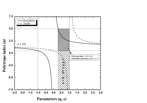
Figure 1: Polytrope index $n$ as a function of the Kaniadakis ($\kappa$) and Tsallis ($q$) parameters. The vertical dotted lines mark the limits of validity of $\kappa$-statistical ($-1\leq\kappa\leq 1$)k01 ; k02 ; k03 ; review ; k10 ; k11 .

In Figure $1$ we display the dependence between the entropic indexes ($\kappa;q$) and the polytropic index ($n$), given by Eqs. (30) and (31), respectively. We show that the polytropic index diverges for the non-Gaussian parameters $\kappa=0,q=1$, i.e., the isothermal spheres separate the polytropes into two branches. For $\kappa>0$ and $q>1$, $n$ ranges from $\infty$ to $3/2$. From $f\sim\mathcal{E}^{n-3/2}$, we see that $\mathcal{E}$ is a decreasing function of the energy and, when $n=3/2$, the distribution function becomes a constant independent of energy. On the other hand, it is well known that, for any astrophysical system, $n$ should be positive and higher than $1/2$ binney87 . Thus the intervals $0\leq q\leq 1$ and $-1\leq\kappa\leq 0$ represent forbidden regions, since the values of $n$ index tend to be smaller than $1/2$ and negative.

It is also worth observing that $\kappa<-1$ and $q<0$ also provides $n>1/2$. However this limits on $\kappa;q$ violates the validity of $\kappa$-statistics k01 ; k02 ; k03 ; review ; k10 ; k11 and the non-extensive $H$-theorem TH , respectively. As is well known, for the polytropic index $n>5$, the density falls off so slowly at large radii that the mass is infinite binney87 . Figure 1 shows that only the branches on the right-side are physically significant for $n<5$. Therefore, the physical values of the Tsallis parameter $q$ should be larger than $9/7$, and the Kaniadakis parameter $\kappa$ should be constrained to interval of validity $\kappa\in[2/7;1]$ represented by the lower dashed rectangle. It is also worth noting that the polytropic indices obtained from Kaniadakis’ statistics are restricted to the range $5/2\leq n\leq 5$, which excludes important stellar polytopes of index $n=3/2$, i.e., the models of adiabatic stars supported by pressure of a non-relativistic gas chandra .

Summing up, a close examination of Figure 1 tells us that the two distributions studied here present a similar behaviour for stellar polytropes, although Kaniadakis function is more restrictive than Tsallis. In reality, in order to know that framework is better, we should do a study based on observational data, e.g., an investigation considering the comparison between Stellar polytropes and Navarro-Frenk-White halo models for the description of dark matter halos (See Ref. navarro ). In this regard, an analysis considering this issue is currently under investigation.

IV Conclusions

In this work we have studied Kaniadakis statistics based on the generalized Maxwellian formulation for the $\kappa$-statistics and, as an application, we investigate the physical effect on the stellar polytropic system. In the first part, we conclude that there is a Kanidakis velocity distribution given by Eq. (16) that is uniquely determined by the requirements of (i) isotropy and (ii) a generalization of the factorizability condition. From the physical viewpoint, this generalization introduces statistical dependence between the velocity components, when we replace the logarithm function by a power law (a similar argument was considered in Refs. TH ; TH1 ; TH2 ; TH3 ; santos11 for the non-Gaussian generalization of molecular chaos hypothesis). In particular, Maxwell expressions are recovered in the Gaussian limit, $\kappa\rightarrow 0$.

From an application perspective, we have shown that the expressions for Tsallis and Kaniadakis, given by Eqs. (31) and (30), present similar behaviours. However, the astrophysical limit on the polytropic index $1/2<n<5$, provides the constraint $\kappa\in[2/7;1]$ and $q>9/7$ for the Kaniadakis and Tsallis parameters, respectively. It is worth mentioning that the Gaussian limit $\kappa=0$, equivalent the Tsallis expression Eq. (31) for $q=1$, reproduces Maxwellian isothermal spheres or, equivalently, $n=\infty$.

- (1) C. Tsallis, J. Stat. Phys. 52, 479 (1988)
- (2) G. Kaniadakis, Physica A 296, 405 (2001)
- (3) G. Kaniadakis, Phys. Rev. E 66, 056125 (2002)
- (4) G. Kaniadakis, Phys. Rev. E 72, 036108 (2005)
- (5) G. Kaniadakis, Eur. Phys. J. B 70 (2009)(special number)
- (6) G. Kaniadakis, Europhys. Lett. 92, 35002 (2010)
- (7) G. Kaniadakis, Phys. Lett. A 375, 356 (2011)
- (8) G. Kaniadakis, Phys. Lett. A 288, 283 (2001)
- (9) G. Kaniadakis, A.M. Scarfone, Physica A 305, 69 (2002)
- (10) G. Kaniadakis, P. Quariti, A.M. Scarfone, Physica A 305, 76 (2002)
- (11) P. H. Chavanis, P. Laurencot, M. Lemou, Physica A 341, 145 (2004)
- (12) F. I. M. Pereira, R. Silva, and J. S. Alcaniz, Nuc. Phys. A 828, 136 (2009)
- (13) G. Kaniadakis, M. Lissia, A. M. Scarfone, Phys. Rev. E 71, 046128 (2005)
- (14) A. M. Teweldeberhan, H. G. Miller, R. Tegen, Int. J. Mod. Phys. E 12, 669 (2003)
- (15) A. Rossani, A. M. Scarfone, J. Phys. A: Math. Gen. 37 4955 (2004)
- (16) M. Cravero, G. Labichino, G. Kaniadakis, E. Miraldi, A. M. Scarfone, Physica A 340, 410 (2004)
- (17) D. Rajaonarison, D. Bolduc, H. Jayet, Econ. Lett. 86 13 (2005)
- (18) A. M. Scarfone, Phys. Rev. E 71, 051103 (2005)
- (19) R. Silva, Eur. Phys. J. B 54, 499 (2006)
- (20) R. Silva, Phys. Lett. A 352 17 (2006)
- (21) G. Lapenta, S. Markidis, A. Marocchino and G. Kaniadakis, Astrophys. Journ. 666, 949 (2007)
- (22) J. C. Carvalho, R. Silva, J. D. Jr. do Nascimento, J. R. De Medeiros, Europhys. Lett. 84, 59001 (2008)
- (23) J. C. Carvalho, J. D. Jr. do Nascimento, R. Silva, J. R. De Medeiros, Astrophys. Journ. Lett. 696, L48 (2009)
- (24) B. B. Soares and J. R. P. Silva, Europhys. Lett. 96, 19001 (2011)
- (25) J. C. Carvalho, R. Silva, J. D. Jr. do Nascimento, B. B. Soares and J. R. De Medeiros, Europhys. Lett. 91, 69002 (2010)
- (26) A. Plastino, A. R. Plastino, Phys. Lett. A 174, 384 (1993)
- (27) A. R. Plastino, Europhysics News 36, 208 (2005)
- (28) J. C. Maxwell, Philos. Mag. Ser. 4, 20, 21 (1860)
- (29) A. Sommerfeld, Thermodynamics and Statistical Mechanics, Lectures on Theorethical Physics, Vol. V, Academic Press, New York (1993)
- (30) R. Silva, A. R. Plastino, J. A. S. Lima, Phys. Lett. A 249, 401 (1998)
- (31) J. Binney and S. Tremaine, Galactic Dynamics, Princeton University Press, Princeton (1987)
- (32) J. A. S. Lima, R. Silva, A. R. Plastino, Phys. Rev. Lett. 86, 2938 (2001)
- (33) S. Chandrasekhar, An Introduction to the Study of Stellar Structure, Dover Publications, New York (1967)
- (34) J. Zavala, D. Núnez, R. A. Sussman, L. G. Cabral-Rosetti, T. Matos, JCAP 06 008 (2006)
- (35) J. A. S. Lima, R. E. de Souza, Physica A 350, 303 (2005)
- (36) R. Silva, J. A. S. Lima, Phys. Rev. E 72, 057101 (2005)
- (37) R. Silva, D. H. A. L. Anselmo, J. S. Alcaniz, Europhys. Lett. 89, 10004 (2010)
- (38) R. Silva, D. H. A. L. Anselmo, J. S. Alcaniz, Europhys. Lett. 89; 59902 (2010) (Erratum)
- (39) A. P. Santos, R. Silva, J. S. Alcaniz, D. H. A. L. Anselmo, Phys. Lett. A 375, 352 (2011)