A model for sequential evolution of ligands by exponential enrichment (SELEX) data

Abstract

A Systematic Evolution of Ligands by EXponential enrichment (SELEX) experiment begins in round one with a random pool of oligonucleotides in equilibrium solution with a target. Over a few rounds, oligonucleotides having a high affinity for the target are selected. Data from a high throughput SELEX experiment consists of lists of thousands of oligonucleotides sampled after each round. Thus far, SELEX experiments have been very good at suggesting the highest affinity oligonucleotide, but modeling lower affinity recognition site variants has been difficult. Furthermore, an alignment step has always been used prior to analyzing SELEX data.

We present a novel model, based on a biochemical parametrization of SELEX, which allows us to use data from all rounds to estimate the affinities of the oligonucleotides. Most notably, our model also aligns the oligonucleotides. We use our model to analyze a SELEX experiment containing double stranded DNA oligonucleotides and the transcription factor Bicoid as the target. Our SELEX model outperformed other published methods for predicting putative binding sites for Bicoid as indicated by the results of an in-vivo ChIP-chip experiment.

abstractwidth281pt

, , , , , , and

t1Joint first authorship. t3Supported in part by NIH-R01GM075312. t4Supported in part by NSERC Grant RGPIN 356107-2009. t5The in vitro and in vivo DNA binding data were funded by the U.S. National Institutes of Health (NIH) under Grant GM704403 (to MDB and MBE). Work at Lawrence Berkeley National Laboratory was conducted under Department of Energy Contract DE-AC02-05CH11231. t6Not affiliated with Lawrence Berkeley National Laboratory now.

1 Introduction

Transcription factors are proteins that regulate gene transcription of DNA by binding to DNA sequence motifs within the genome. Mapping these DNA recognition sequences and determining the relationship between DNA sequence and transcription factor binding affinity is central to understanding the regulation of gene expression. Transcription factors comprise approximately 8% of the genes encoded in the human genome. A comprehensive understanding of the behavior of these proteins will aid in our understanding of key developmental processes, including body patterning, brain development and tissue specification.

One in-vitroassay, known as Systematic Evolution of Ligands by EXponential enrichment (SELEX), indirectly measures the affinity of a transcription factor binding to various DNA sequences. SELEX was introduced in the 1990s by Tuerk and Gold (1990) and Ellington and Szostak (1990). It has been used in a number of genomic studies [e.g., Kim et al. (2003) and Freede and Brantl (2004)] and for the purposes of drug discovery [e.g., Guo et al. (2008) and Ng et al. (2006)]. In genomic studies, SELEX has been used to identify the highest affinity recognition sequences for target proteins.

More recently there has been an emphasis on using SELEX data to estimate not just the highest affinity sequences but also a matrix for the free energy of binding. Using the free energy matrix, one can build a model which takes as input a nucleotide sequence and outputs the affinity of the sequence for the transcription factor. With a flexible model, one can scan the genome to find high to medium affinity putative binding sites. Having such a model is important since the nucleotide sequence with the highest affinity for the transcription factor might not be occupied in-vivo. For instance, due to DNA folding and histone interference, the highest affinity site may be inaccessible to the transcription factor. Also, the specificity of the site may play a role. That is, a medium affinity site surrounded by very low affinity sequences might be a functionally more important binding site than a high affinity site surrounded by other high affinity sites. Such requirements have led researchers to consider thermodynamic models for SELEX. Djordjevic and Sengupta (2006) and Zhoa, Granas and Stormo (2009) are two thermodynamic models for SELEX that precede ours. We will clearly illustrate how our model diverges from Djordjevic and Sengupta (2006) and Zhoa, Granas and Stormo (2009) in Sections 2 and 3 after we describe the SELEX experiment in detail.

Our model is a result of a large collaboration, the Berkeley Drosophila Transcription Network Project (BDTNP). The goal of the BDTNP is to understand the early developmental transcription factors in fly embryos. As part of this collaboration, in-vitro SELEX, in-vivo ChIP-chip and, most recently, in-vivo ChIP-seq have been performed on many transcription factors. Although the in-vivo ChIP-seq results are extremely important because they identify regions along the genome to which a transcription factor actually bound at an instant in time in a particular developmental stage in a specific tissue or cell lineage, we believe that the in-vitro SELEX experiment is still extremely relevant for two reasons.

First, the ChIP-seq assay is exceedingly expensive, currently at a minimum cost of $\$5\mathrm{K}$ per sample. To fully understand a developmental process, it would be necessary to conduct ChIP-seq in every tissue or cell lineage in an animal throughout its development. At $\$5\mathrm{K}$ per sample this cost is already prohibitive before we even account for the manpower required. The in-vitro binding data from SELEX allows us to reason about all locations in a genome that might be bound by the transcription factor of interest in any sample. Obviously, this can be very powerful when combined with information from other in-vivo assays, such as DNasel accessibility experiments [Li et al. (2011) and Kaplan et al. (2011)].

Second, there is great value to obtaining the qualitative, thermodynamic estimates of protein/DNA binding affinities that we model in this paper from SELEX data. Ultimately, biologists would like to understand the relationship between transcription factor binding patterns and gene expression [Ay and Arnosti (2011)]. Transcription factors have been shown to work together in complex spatial arrangements in order to modulate gene expression [Biggin (2011)] and the dynamics of these spatial configurations and their effects on transcription initiation can not be observed by ChIP-seq or any other widely utilized assay. Such critical aspects of gene regulation can, at present, on a large scale, be inputted only computationally, using models of protein/DNA binding affinities [Ravasi et al. (2010), Boyle et al. (2010) and Kaplan et al. (2011)]. Therefore, models such as the one we propose here based on SELEX data will continue to be an important area of computational biology for the foreseeable future.

2 The SELEX assay and likelihood for the model

A typical SELEX experiment begins in round one with a solution of random double stranded DNA oligonucleotides and a transcription factor. In the application presented in this paper the oligonucleotides are 16 base pairs long sequences and are flanked by additional DNA sequences.

The oligonucleotides react with the transcription factor and eventually a dynamic equilibrium is reached where the concentrations of bound oligonucleotides, unbound oligonucleotides and unbound target are constant. After equilibrium is reached, the bound oligonucleotides are separated from the solution. Next, a polymerase chain reaction (PCR) is performed on the oligonucleotides sampled from the end of round one. PCR chemically amplifies the quantity of DNA present in a way that does not significantly change the frequency distribution of oligonucleotides. At this point, a sample is taken for sequencing, and the remaining oligonucleotides are entered into round two. The main steps for round one of SELEX are depicted in Figure 1.

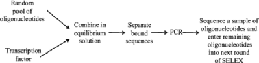
Figure 1: The main experimental steps for round one of a SELEX experiment.

Round two of SELEX proceeds exactly as round one, except that the initial pool of oligonucleotides is the set of bound oligonucleotides from round one that went through PCR but were not sequenced. Thereafter, the assay proceeds as before: the oligonucleotides react with the transcription factor and, after equilibrium is reached, the bound oligonucleotides are selected and PCR is performed. A sample is taken for sequencing and the remaining oligonucleotides are entered into round three. These steps are repeated for as many rounds as the experimenter desires; see Ogawa and Biggin (2011) for full experimental details.

The outcome of a SELEX experiment is observed by sequencing the oligonucleotides that are sampled at the end of each round. That is, after performing the assay, the results are a list of sequenced oligonucleotides and usually meta-data, such as the SELEX round in which each oligonucleotide was sequenced, the concentration of unbound transcription factor in a particular round, and/or the temperature at which the experiment was performed.

Each sequence is denoted by $S_{i}$, where $i$ enumerates over all the different sequence types. Letting $k$ represent the length of the sequences and carefully accounting for palindromes and reverse palindromes, for our double stranded DNA application $i=1,\ldots,n$ where $n=2^{k-1}+4^{k-1}$. We let $r$ identify the round number beginning with $r=0$ for the initial random pool of sequences. The number of times sequence type $S_{i}$ is observed in round $r$ is represented by $l_{i,r}$. Table 1 shows the first ten 16mers $S_{i}$ and the number of times each sequence appeared $l_{ir}$ in round $r=3$ of a SELEX experiment for the transcription factor Bicoid. Although we only show ten sequences, a total of $1324$ unique sequences $S_{i}$ were observed in round 3 of the SELEX experiment depicted in Table 1.

=220pt $\bolds{S_{i}}$ $\bolds{l_{i,3}}$ TCCCATTAATCCCACC 2 GGTGTCGGTTTAAGCG 2 CTGATTAATCCGAGTG 1 TGAGATTCCATACCCT 1 TGTGAGGATATGTTTC 1 TGGGGTTGGATTAAAG 1 GGATTAGGGTTAAGCA 1 GACCCCGGCCTAATCC 1 GGTAATCTCGGGATTA 1 TGGACGGATTACGCGG 1

Table 1: Example of first ten sequences $S_{i}$ and their frequencies $l_{i,3}$ collected after the third round of a SELEX experiment for the transcription factor Bicoid

A complicating factor of SELEX is that the length of the binding site $l$ to the transcription factor is less than the length of the sequences $k$. In the application of this paper we have $k=16$ and we estimate the binding site length of Bicoid $l$ to be at most $10$. All previous methods, including Djordjevic and Sengupta (2006) and Zhoa, Granas and Stormo (2009), for analyzing SELEX data use an alignment step prior to analyzing the SELEX data. Such aligners [e.g., Multiple Em for Motif Elicitation (MEME), Bailey et al. (2006)] are not based on the thermodynamics of binding. For each kmer, these aligners will output their “best guess” for the lmer to which the sequence $S_{i}$ is bound. We denote the lmer binding sites by $b_{j}$. For example, Table 2 shows ten aligned sequences from a SELEX experiment for the transcription factor Bicoid. The sequences are aligned for a binding site of $l=8$ using an aligner written in the Biggin lab by Stuart Davidson.

=220pt $\bolds{b_{j}}$ ATA TTAATCCG ATAAC CACCC TAAATCTT CGT TTAATCCA GCGCATCA ACCC TTAATCCC CCCA CAACC TTAATCCC TAA TCCCTCCT AATCC T TTAATCCT GATCCCC GGA TTAACTCG GATTA GAGAGG TTAATCCA CT GTAC CAAGTCAC CACA

Table 2: Ten aligned sequences from a SELEX experiment for the transcription factor Bicoid. The sequences here were aligned assuming a binding site of length $l=8$

Previous models for SELEX take the estimated binding site sequences $b_{j}$ from an aligner as input. Our model selects binding sites dynamically as part of the optimization. That is, the model takes the full kmer $S_{i}$ sequences that were sequenced after each round of the SELEX experiment as input. The likelihood (1) is parametrized in terms of $P_{r}(S_{i})$, where $P_{r}(S_{i})$ denotes the probability of selecting sequence $S_{i}$ in round $r$. In Section 3 we provide the parametrization for $P_{r}(S_{i})$ in terms of the free energy, $\Delta G$, a thermodynamic measure of affinity. Letting $R$ denote the total number of rounds for the SELEX experiment, we have

$$L(\Delta G|l_{11},\ldots,l_{nR})=\prod_{r=1}^{R}\Biggl{(}\prod_{i=1}^{n}P_{r}(S_{i})^{l_{ir}}\Biggr{)}.$$ (1)

It is easily seen from the likelihood (1) that our model for SELEX can take as input data from all rounds of a SELEX experiment. This is important, as there is evidence that a range of affinities is required to properly estimate the free energy, $\Delta G$ [see the review article Djordjevic (2007)]. Our model for SELEX is the first model to use data from all rounds of the experiment; previous models use only data from the last round which consists of high affinity sequences.

3 Parametrization of the model

Section 3.1 describes how the probability of a sequence $S_{i}$ binding to the transcription factor in round $r$, $t_{r}(S_{i})$, is parametrized in terms of the Gibbs free energy $\Delta G$. Section 3.2 provides the parametrization of the probabilities $P_{r}(S_{i})$ of drawing $S_{i}$ from round $r$. Appendix A gives the necessary chemical background.

3.1 Probability of a sequence $S_{i}$ binding

In SELEX, we have multiple oligonucleotide types $S_{i}$ in solution. At dynamic equilibrium in round $r$, the probability of any copy of type $S_{i}$ being bound at a particular instant is equal to the fraction of $S_{i}$, that is, bound, $t_{r}(S_{i})$. Letting $[\mathit{TF}\dvtx S_{i}]_{r}$ and $[S_{i}]_{r}$ represent the long term average concentrations of the bound product and unbound sequences $S_{i}$ in round $r$, we have

$$t_{r}(S_{i})=\frac{[\mathit{TF}\dvtx S_{i}]_{r}}{[\mathit{TF}\dvtx S_{i}]_{r}+[S_{i}]_{r}}.$$ (2)

We are interested in modeling the affinity of oligonucleotides that bind in a sequence specific manner to the target. Specific binding involves hydrogen bonding, van der Waals interactions and other short-range forces. Sequence independent binding also occurs. This is due in part because oligonucleotides bind weakly via electrostatic forces [see von Hipple (2007)], and because a small percentage of DNA will nonspecifically associate with the bead or non-DNA binding surfaces of the target. Thus, even oligonucleotides that do not bind to the target specifically can be present in later rounds. We make three assumptions concerning specific binding for any oligonucleotide type $S_{i}$:

[1.]

All identical copies of the same oligonucleotide type $S_{i}$ bind at the same subsequence $b_{j}$. We refer to this subsequence as the binding site.

The subsequence $b_{j}$ is assumed to be of fixed length $l$ and independent of the oligonucleotide type $S_{i}$ in which it is contained.

The binding site $b_{j}$ for each oligonucleotide type $S_{i}$ is that subsequence which has maximum affinity according to the proposed model. These correspond to the assumptions that the binding affinity of the sequence is solely a function of the binding site and that there is only one binding site per oligonucleotide.

Given these assumptions and letting $[\mathit{TF}]_{r}$ represent the long term average concentration of unbound transcription factor at dynamic equilibrium in round $r$, we can use (8), (11) and (2) to write

$$t_{r}(S_{i})=\frac{[\mathit{TF}]_{r}\exp({(-\Delta G(S_{i}))}/{(R_{\mathrm{Gas}}T)})}{1+[\mathit{TF}]_{r}\exp({(-\Delta G(S_{i}))}/{(R_{\mathrm{Gas}}T)})},$$ (3)

where $\Delta G(S_{i})\equiv\Delta G(b(S_{i}))$ and $b(S_{i})$ maximizes $\Delta G$ among all $b_{j}$’s of the length $l$ we have specified contained in $S_{i}$.

In a SELEX experiment, $t_{r}(S_{i})$ can also be viewed as the conditional probability that a particular molecule of the species $S_{i}$ is bound at the end of round $r$ given that it is present at the beginning of round $r$. Formally,

$$t_{r}(S_{i})\equiv P[S_{i}\mbox{ bound at the end of }r|\mbox{it is present in }r].$$ (4)

Defining $\widehat{[\mathit{TF}]}_{r}$ to be the concentration of the transcription factor at a particular instant, we obtain $\widehat{t_{r}}(S_{i})$,

$$\widehat{t_{r}}(S_{i})=\frac{\widehat{[\mathit{TF}]_{r}}\exp({(-\Delta G(S_{i}))}/{(RT)})}{1+\widehat{[\mathit{TF}]_{r}}\exp({(-\Delta G(S_{i}))}/{(RT)})},$$ (5)

which is an estimate of $t_{r}(S_{i})$. We expect that the instantaneous concentrations $\widehat{[\mathit{TF}]}_{r}$, $\widehat{[\mathit{TF}\dvtx S]}_{r}$ and $\widehat{[S]}_{r}$ will vary within $5\%$ of their long term average concentrations $[\mathit{TF}]$, $[\mathit{TF}\dvtx S]$ and $[S]$.

It is very difficult to measure the amount of transcription factor that is “active” in a binding reaction, versus denatured or otherwise nonfunctional. Hence, we do not have measurements for $\widehat{[\mathit{TF}]_{r}}$ and this causes an identifiability problem when estimating $\Delta G$. The problem is easily remedied by estimating $\Delta\Delta G$ instead. See Appendix B.1 for further discussion.

Although the notation differs, our formulation for the probability of a sequence type $S_{i}$ binding in round $r$, $\widehat{t_{r}}(S_{i})$, resembles the parametrization first introduced by Djordjevic and Sengupta (2006) and later used by Zhoa, Granas and Stormo (2009). The thermodynamic formulation (3) includes competitive binding between oligonucleotides $S_{i}$ since the $S_{i}$ are all competing for the unbound transcription factor. As we search all possible binding sites of each oligonucleotide type $S_{i}$ for the optimal site, our model takes alignment into account implicitly, unlike Djordjevic and Sengupta (2006) and Zhoa, Granas and Stormo (2009) which either use a pre-alignment step as in Table 2 or work on data with $k=l$.

3.2 Probability of drawing a sequence $S_{i}$

Next we express the distribution of bound sequences in terms of (5). We first assume that each sequence is present in an initial amount $C_{0}$ in round zero. We then make the assumption that each PCR step replicates each molecule of type $S_{i}$ $A_{r}$ times on average in round $r$. Then, after the $r$th round of selection the amount of $S_{i}$ is

$$C_{0}\prod^{\bar{r}}_{r=1}A_{r}\widehat{t_{r}}(S_{i}).$$

Dividing the total amount of $S_{i}$ after round $\bar{r}$ by the total amount of all sequences after round $\bar{r}$ gives an estimate of the frequency distribution of bound sequences at the end of round $\bar{r}$. Formally,

$$\qquad P_{\bar{r}}(S_{i})=P[S_{i}\mbox{ is sequenced in round }\bar{r}]=\frac{\prod_{r=1}^{\bar{r}}\widehat{t_{r}}(S_{i})}{\sum_{\mathrm{all\ }S_{j}}\prod_{r=1}^{\bar{r}}\widehat{t_{r}}(S_{j})}.$$ (6)

Djordjevic and Sengupta (2006) assume that all the sequences they see in the last round bound the protein and all the sequences they do not see did not bind. Hence, their likelihood differs significantly from ours. Like us, Zhoa, Granas and Stormo (2009) account for the multinomial sampling in (6). Zhoa, Granas and Stormo (2009) also account for extra variability generated during amplification by PCR. Both Zhoa, Granas and Stormo (2009) and us fail to correct for the case in which zero oligonucleotides of a particular species are bound in round $r$. The large oligonucleotide counts makes this a reasonable approximation. For instance, in the data we study in Section 5, each 16mer species had an average of 65,000 copies in round zero.

As discussed in Section 3.1, it is possible for oligonucleotides to make it though the selection step via a variety of mechanisms, including nonsequence mediated, electrostatic protein–DNA interaction (nonspecific binding), DNA–DNA interactions or DNA–apparatus interactions (experimental error). We account for such sequences in our model, and refer to the effects that result in their selection collectively as Junk Binding. If $c_{J}$ is a constant between $0$ and $1$, then we can modify our equations to allow for junk binding as follows:

$$\widehat{t_{r}}(c_{J},S_{i})=\bigl{(}(1-c_{J})\widehat{t_{r}}(S_{i})+c_{J}\bigr{)}.$$

Our parametrization of the junk binding is different from Djordjevic and Sengupta (2006) and Zhoa, Granas and Stormo (2009) who both use only a thermodynamic parametrization for the nonspecific binding.

3.3 Binding model

The binding model is the relationship between the actual DNA sequence of a binding site $b_{j}$ and the free energy $\Delta G$. So far we have formulated our model in complete generality with respect to the binding model. The most widely applied model is an additive one. The additive model was used in both Djordjevic and Sengupta (2006) and Zhoa, Granas and Stormo (2009). Such a model assumes that each base pair of DNA makes some contribution to the total binding affinity independent of all other base pairs in the binding site. Representing the nucleotide base pair at position $k$ in $b_{j}$ as $o_{k}$, and letting $\varepsilon_{t}(o_{k})$ represent the indicator function

$$\varepsilon_{t}(o_{k})=\cases{1,&\quad$\mbox{if }o_{k}=t,$\vspace*{2pt}\cr 0,&\quad$\mbox{otherwise},$}$$

we write the elements of the energy matrix as $\lambda_{kt}$,

$$\Delta G(b_{j})=\sum_{k=1}^{l}\sum_{t\in\{A,C,G,T\}}\lambda_{kt}\varepsilon_{t}(o_{k}).$$ (7)

As before, the length $l$ represents the length of the binding site. The parameters to be estimated are the $\lambda_{kt}$ from the energy matrix.

It is important to note that our additive model (7) does not correspond to a Position Weight Matrix (PWM). In a PWM the nucleotide positions are treated independently. In our notation this means that the probability of sequence $S_{i}$ binding to the transcription factor, $t_{r}(S_{i})$, will equal a product of probabilities where each probability corresponds to a position in the sequence and the value of each probability is determined by the nucleotide at the corresponding position. Our model deviates from such an independence model in two important ways:

• By assuming that the binding of a sequence is determined by a smaller binding site, our model permits considerable dependence between nucleotide positions and sequences well separated in hamming distance. If we group the sequences by the binding sites that give minimal free energy, we see that the distribution of binding probabilities over sequences is a mixture of probability distributions, each of which, ignoring thermodynamic considerations, could be characterized by PWM.

• Even when the sequence and binding site coincide, that is, when $k$ and $l$ are equal, the probability of a sequence $S_{i}$ binding $t_{r}(S_{i})$ is modeled by a log odds model. Rearranging equation (5),

  $$\log\biggl{(}\frac{t_{r}(S_{i})}{1-t_{r}(S_{i})}\biggr{)}=\log([\mathit{TF}]_{r})-\frac{\Delta G(S_{i})}{RT}.$$

4 Optimization

This section discusses the optimization of our model. In particular, Section 4.1 explains how we simulate to simplify the denominator of $P_{r}(S_{i})$ and Section 4.2 discusses the numerics of the optimization procedure. There are three identifiability issues with our model that are easily overcome. The identifiability issues are presented in Appendix B.

4.1 Denominator of $P_{r}(S_{i})$

For $k=16$ the number of oligonucleotide types in the initial random pool is $2^{15}+4^{15}$. It is infeasible to include all oligonucleotide types in the denominator of (6). We estimate the denominator using Monte Carlo and take a simple random sample of oligonucleotides by selecting nucleotide base pairs from a uniform distribution. Our approach differs from Zhoa, Granas and Stormo (2009) who discretized the energy distribution in order to simplify the denominator before numerically optimizing to estimate the free energy matrix $\Delta G$.

4.2 Numerical optimization

With regards to our model, a point not yet discussed is the difficulty of maximizing the likelihood. If $[\mathit{TF}]_{r}$ is “small,” then the denominator in (5) can be approximated by one. The likelihood (1) will simplify, and the optimization between each alignment step becomes a convex optimization problem. However, since we avoid making simplifications regarding the concentration of a transcription factor in each round, the optimization is more difficult, as discussed below.

There are substantial computational and algorithmic difficulties in fitting the model. Standard optimization techniques are often ineffective because the likelihood surface is neither convex nor differentiable. In particular, the lack of continuous derivatives makes gradient descent methods like Broyden–Fletcher–Goldfarb–Shanno (BFGS) [Nocedal and Wright (2006)] unstable. In addition, the lack of convexity means that line search methods [Nelder and Mead (1965)] tend to become trapped in local maxima. In view of these considerations, we have had success using downhill simplex methods [Powell (1964)] from a large set of random starting locations. This method is, empirically, stable. The software tool presented in the supplementary material [Atherton et al. (2012)] implements this method. The simulations and results in Section 5 were all produced using the provided software tool.

5 Results

In Section 5.1 we demonstrate how our model works on simulated data. Section 5.2 applies our model to Bicoid SELEX data from the Biggin Lab. We then compare the estimates from our model to estimates made from an in-vitro multiplex assay experiment in the Biggin Lab and to estimates made from the Binding Energy Estimates using the Maximum Likelihood (BEEML) model of Zhoa, Granas and Stormo (2009) in Section 5.3.

Table 3: The Gibbs free energy matrix estimated from a SELEX experiment on the transcription factor Bicoid

	A	C	G	T
1	$-4.722516$	$-5.729347$	$0.000000$	$-6.251779$
2	$-7.447426$	$-5.981440$	$0.000000$	$-16.853690$
3	$0.000000$	$-6.946246$	$-15.701235$	$-8.529272$
4	$-7.746046$	$-15.548042$	$-12.535315$	$0.000000$
5	$-7.989755$	$-7.201358$	$-24.708969$	$0.000000$
6	$0.000000$	$-9.611195$	$-8.497223$	$-5.336888$
7	$-0.505663$	$-19.926999$	$0.000000$	$-4.445374$
8	$-1.836787$	$-0.228140$	$0.000000$	$-0.945140$
9	$-1.841359$	$-1.612913$	$0.000000$	$-1.417988$
10	$-1.431632$	$-1.539663$	$0.000000$	$-0.235633$

Finally, we see how our model performs versus other published methods when searching for transcription factor binding sites along the genome. In Section 5.4 we observe that for the transcription factor Bicoid there is good agreement between the putative binding sites predicted by an in-vivo ChIP-chip experiment performed in the Biggin Lab and all the other published methods we compare it with; however, the agreement is strongest between the ChIP-chip experiment and the results of our model applied to the SELEX data for Bicoid.

We have chosen to explain the results from Bicoid in detail because it has been studied extensively in the literature and we have multiple replicates of the SELEX experiment, the multiplex assay experiment and the ChIP-chip experiment. The protocol for the SELEX experiment is provided in Ogawa and Biggin (2011).

5.1 Simulations

To explore the properties of our estimation procedure, we simulated data under our model and refit the model parameters from the simulated data. The energy model that we simulated under is a plausible model for binding of the Bicoid homebox which is strongly attracted to sequences that include TAAT. In fact, the energy matrix used for the simulation is the matrix estimated in Table 3.

To simulate data under the SELEX model, we generated one million 16mer random sequences uniformly, which we refer to as round 0. Then, for rounds $r=1,\ldots,4$, we keep each sequence in round $r-1$ with the probability given by (3).

To simulate the PCR duplication process, in which the number of oligonucleotides is typically much larger than the number of PCR molecules, we repeatedly selected a sequence at random and duplicated the selected sequence, until we had one million sequences.

After we had reached one million sequences, we randomly sampled $2000$ of these without replacement. The $2000$ sequences are the data for round $r$, which we fed into our model. The other sequences formed the selection pool for round $r-1$.

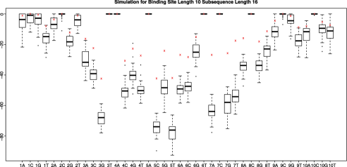
Figure 2: Boxplots of the free energy parameters estimated from the $32$ simulations. The values that generated the simulations are shown by red crosses.

In Figure 2 we present boxplots of the estimated parameter values for $32$ simulations. We simulate our Bicoid SELEX data situation of having a binding site length of $l=10$ inside random $16$mer sequences $S_{i}$. As can be seen, under the model, our procedure provides biased results. In our simulations, the binding strength of the consensus sequence is overestimated. We believe this bias will also be present but hopefully smaller in magnitude when real SELEX data is analyzed, since a real SELEX experiment will begin in round 0 with many, many more sequences that 1 million. To the best of our knowledge, the bias is present due to the fact that we assume in our model that every sequence type $S_{i}$ is present in each round $r$ of the SELEX experiment. In reality, of course, and in our simulations, weaker sequences will not make it to later rounds of SELEX. This will make the consensus sequence look stronger than it really is.

Many more simulations are provided in the supplementary material [Atherton et al. (2012)]. It appears that as the stringency of the experiment is increased (either by decreasing the amount of the transcription factor or by increasing the energy matrix) the bias is increased. Also seen in our simulations in the supplementary material [Atherton et al. (2012)] is that the bias is also present and much bigger in magnitude in the BEEML model. Of course, the BEEML model makes the same assumption as us that every sequence type is present in each round of SELEX.

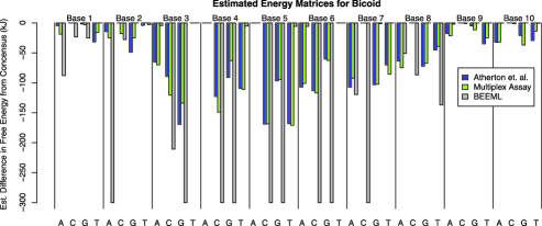
Figure 3: Estimated $\Delta\Delta G$ matrices from (1) a multiplex assay experiment from the Biggin Lab (green), (2) our model applied to all four rounds of a SELEX experiment for Bicoid (blue), and (3) the BEEML model of Zhoa, Granas and Stormo (2009) applied to data from rounds three and four of the same SELEX experiment for Bicoid (grey).

Unfortunately it is impossible to know exactly what sequence types are in each round $r$ of a SELEX experiment. Since we wanted to include data from all rounds of a SELEX experiment and include alignment in our model, we are forced to assume that all possible sequence types are present in every round. In our earliest efforts to model SELEX data we used models which only included the last round of SELEX and we assumed that the only binding sites $b_{i}$ that were present were the binding site types that were observed. Of course these models required a pre-alignment step and could only accept data from the last round of SELEX.

5.2 Bicoid SELEX data

Our SELEX model was run on output from all four rounds of the Bicoid SELEX experiment. Here $k=16$ and $l=10$. The $\Delta\Delta G$ matrix is given in Table 3. The sequence with the highest affinity to Bicoid is called the consensus sequence. Our consensus sequence is GGATTAGGGG (or equivalently CCTAATCCCC). We have set the energy of the consensus sequence to be $0$ in Table 3.

5.3 Comparison to the multiplex assay experiment and BEEML

In addition to SELEX, the Biggin Lab has also produced an in-vitro multiplex assay experiment. In this multiplex assay experiment a small number of sequence types $S_{i}$ are produced. Usually the consensus sequence is known a priori (e.g., from a SELEX experiment) and the sequence types $S_{i}$ produced for the experiment vary from the consensus sequence at one or two positions only. As in the SELEX experiment, the $S_{i}$ are entered in solution with the transcription factor Bicoid. The solution is allowed to reach equilibrium and then the bound sequences are separated from the transcription factor. Since there are very few sequence types $S_{i}$ present in this experiment, one can obtain a much more accurate measure of the amount of bound $S_{i}$ than in a SELEX experiment. Using the thermodynamic concepts presented in this paper, one can easily use the measured amounts of each bound sequence type to directly calculate a $\Delta\Delta G$ matrix. The results of the multiplex assay experiment described above for Bicoid are shown in green in Figure 3.

To compare our model to the BEEML model of Zhoa, Granas and Stormo (2009), we had to pre-align the sequences $S_{i}$ for a binding site of length ten. To do the alignment, we used MEME [Bailey et al. (2006)]. We considered using MEME to directly align the sequences and then input these sequences into the BEEML model; however, when aligning sequences MEME clusters like sequences together and also eliminates sequences which do not fit according to their model. Hence, we decided it was preferable to run MEME and construct a mean PWM based on the output from round four of the SELEX experiment. We then used the PWM to find the highest affinity subsequence of length ten in each 16mer $S_{i}$ from rounds three and four of the SELEX experiment. These subsequences were the aligned binding sites that were given to the BEEML model as input. The results of BEEML are shown in grey in Figure 3.

Finally, as described in Section 5.2, we ran our model on all rounds of a SELEX experiment for Bicoid. The results are plotted in Figure 3 in blue.

From Figure 3 we see that the consensus sequence for the multiplex assay experiment is CTTAATCCCC and the consensus sequence for BEEML is TGTAATTGGG. Recall from Section 5.2 that the consensus sequence for our model is CCTAATC CCC. It is clear that all three models pick up the TAAT homebox which is clearly the most important factor in determining the affinity of a subsequence to Bicoid. Also seen from Figure 3 is how deleterious a mutation in the homebox is to binding. Any mutation from TAAT at positions three to six leads to a very substantial decrease in $\Delta\Delta G$. All models show that mutations from the consensus sequence at positions nine and ten are not very critical to binding. The three models also indicate that positions one and two are weakly critical to binding; however, BEEML indicates it is deleterious to have nucleotide base A at positions one and two, whereas our model and the multiplex assay do not show the same deleterious effect. There are other obvious instances where the BEEML model deviates significantly from our model and the multiplex assay experiment.

As for why the BEEML model deviates quite a bit from our model and the multiplex assay experiment for certain nucleotide estimates at certain locations, a main reason is most likely the need to pre-align using MEME, that is, the output we see for BEEML will be heavily influenced by MEME. Our model aligns during the optimization of the likelihood and, hence, unlike MEME, our alignment is based on thermodynamic principles. There are also important differences between BEEML and our model. Both BEEML and our model are thermodynamic models run on the same SELEX experiment, however:

• BEEML accounts for the nonspecific energy of binding. Although our model can account for the nonspecific binding, in this instance, it was run without accounting for nonspecific binding.

• BEEML accounts for errors in the PCR step. We have chosen not to account for that explicitly in our model.

• BEEML also has an expression similar to our expression (6) for $P_{r}(S_{i})$. The problem both models encounter is that there are too many terms to enumerate in the denominator. As described in Section 4.1, we use Monte Carlo to overcome this. The BEEML model takes a different approach similar to Djordjevic and Sengupta (2006) where they discretize over a user defined number of energy levels.

• Our model uses data from all rounds of the experiment. Furthermore, we carefully model the sequence enrichment from one round to the next. The code for BEEML accepts data from two rounds of SELEX, however, there is no indication in Zhoa, Granas and Stormo (2009) that they correctly model the progression from one round to the next.

• The final likelihoods for our model and BEEML are different and optimization schemes used are also different.

Hence, although the BEEML model has offered significant improvements to the original Djordjevic and Sengupta (2006) model, we believe that our model offers further important improvements.

Of course, we also see that our model estimates deviate slightly from the multiplex assay estimates and we hope that in these instances our model is providing good estimates for the $\Delta\Delta G$ matrix since we are using data from many, many more sequence types $S_{i}$ than the multiplex assay experiment. In particular, we are including sequences with a full range of affinities from low to high.

As the $\Delta\Delta G$ energies from the multiplex assay are calculated directly from the thermodynamic equations, we do not anticipate a big bias in the multiplex assay estimates. There does not seem to be any consistent difference between our model estimates of $\Delta\Delta G$ and the estimates from the multiplex assay experiment. This observation supports our hypothesis that the bias observed in our SELEX simulations will be reduced when our model is applied to real data since in a real SELEX experiment there are many more sequences present and, hence, many more low affinity sequences will make it through to later rounds than in our simulation. Basically, we think that the assumption of each sequence type being present in each round is more valid in the real data situation than in the simulated data situation.

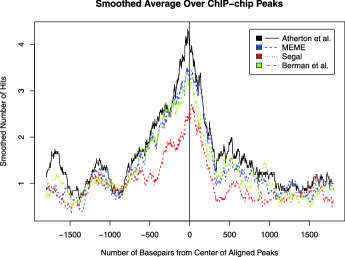
Figure 4: Smoothed average of predicted binding sites for four models at ChIP-chip peaks. The legend is as follows: Atherton et al. represents the model discussed in this paper, MEME represents Bailey et al. (2006), Segal represents Segal et al. (2006) and Berman et al. represents Berman et al. (2004). The fixed parameters (as described in Appendix C) for the analysis of the ChIP-chip data are $n_{p}=100$, $w_{s}=4000$, $n_{s}=100$, and $s_{t}=0.999$. The peaks are aligned so that the center of each peak, defined as the highest point in the peak, appears at $0$ on the $x$-axis.

5.4 Comparison in an in-vivo setting

Using the $\Delta\Delta G$ matrix estimated by our model on the Bicoid SELEX data in Table 3, we scan the genome of Drosophila Melanogaster and compare the results of our model and three other popular models to the results of an in-vivo ChIP-chip experiment.

The Berkeley Drosophila Transcription Network Project (BDTNP) has generated SELEX and ChIP-chip data for Bicoid. ChIP-chip data measures the genome wide relative levels of occupancy for a single protein of interest. We used the BDNTP ChIP-chip data and a simple, nonparametric method to validate and compare our Bicoid model with a PWM derived from MEME [Bailey et al. (2006)] and two models from the literature [Segal et al. (2006) and Berman et al. (2004)]. All four methods show strong agreement with the in-vivo ChIP-chip data, however, our model has the strongest agreement; see Figure 4.

The ChIP-chip experiments identified thousands of genomic regions to which Bicoid binds. This data has been shown to provide a quantitative measure of relative occupancy. That is, regions can be assigned a score, and those scores have been shown to be reproducible between biological replicates [Li et al. (2008) and MacArthur et al. (2009)]. From these and other observations, the authors concluded that the high scoring regions correspond to those with the highest net occupancy of bound factor.

Because of the complexity of intracellular processes, a binding model alone does not provide enough information to predict the results of a ChIP-chip experiment. For instance, without additional data, we have no way of modeling the inhibitory affect of chromatin structure. However, we can still use the identified binding regions to test the validity of our SELEX model and data.

If a binding model is identifying true in-vivo binding sites, then we expect the number of high affinity sites predicted by our model to be higher near ChIP-chip peaks. Roughly, we compared the binding models by measuring the enrichment of identified binding sites as compared to the genomic background. There were several variables that we controlled for; we explain the method in detail in Appendix C. We plotted the results of this analysis for our model and competing models in Figure 4.

Absent from our comparison in Figure 4 is the Zhoa, Granas and Stormo (2009) model. Since, as discussed in Section 5.3, we have to pre-align the sequences of the SELEX experiment using MEME, the output in Figure 4 after transformation by the sequence ranks will be very near to the output of MEME presented in Figure 4.

6 Conclusion

The model presented here attempts to infer a comprehensive map of the sequence specific binding affinities between double stranded DNA and a transcription factor from a SELEX experiment. There exist a variety of assays, including ChIP-chip, that attempt to measure the average binding behavior of a protein in a population of cells. However, only in vitro assays like SELEX can provide precise thermodynamic models of protein/DNA interactions for downstream models of transcriptional control.

To make accurate inference from SELEX data, researchers have left the traditional empirical approaches such as PWMs and recently turned to creating models for SELEX based on the physical chemistry of binding. The goal of these models is to estimate the free energy of binding, $\Delta G$, matrix. Often the exact binding site length $l$ is unknown a priori, hence, SELEX experiments are performed with a sequence length $k$ greater than $l$. Also, by taking a large $k$, as in the Biggin Lab, once a random pool of sequences has been generated, SELEX experiments can be performed for many transcription factors with varying binding site lengths $l$. Our model for SELEX is the first model capable of accepting data of the form $k>l$. Other models for SELEX can only accept data with $k=l$ or require an alignment step a priori. Another important feature of our model is that it accepts data from all rounds of the SELEX experiment. This is crucial for estimation of $\Delta G$, since a mix of oligonucleotides that have a range of affinities for the transcription factor are required. Previous models only use data from the last round of the SELEX experiment and hence base their estimates on oligonucleotides with a high affinity to the transcription factor.

The success of our model is demonstrated by applying our model and three others to predict the DNA recognition sites enriched in an in-vivo ChIP-chip experiment. The in-vivo ChIP-chip experiment indicates the in-vivo occupancy of the transcription factor along the genome. A prior, it may not have been the case that the affinity of a sequence for a transcription factor as measured in an in-vitro experiment is a good predictor for binding sites occupied in-vivo, even after taking into account of the influence of other proteins, such as nucleosomes, on occupancy in vivo. However, we have found that for the transcription factor Bicoid the recognition sites used in-vitro and in-vivo are very closely related. Hence, we can use the in-vivo ChIP-chip experiment as validation when comparing different models and motifs for binding. It is important that a comparison of models be made with the ChIP-chip experiment, as this can serve as a gold standard for binding affinity; otherwise, finding that two models produce different motifs or different energy matrices is insufficient to determine which model is performing better. Our success using results from an in-vivo experiment to validate the results of an in-vitro experiment suggests that SELEX does provide a quite accurate, fine scale model of the intrinsic DNA recognition properties of a transcription factor. The results of our comparison in Section 5.4 demonstrate that our model outperforms the other models.

Preliminary results suggest that varying the additive $\Delta G$ parametrization of our model would provide the biggest predictive improvement. For instance, base pair dependencies can be added. Alternatively, one could take a feature based approach; see Sharon, Lubliner and Segal (2008). In the case of Bicoid, a feature based approach could specifically model the TAAT homebox.

Appendix A Chemical concepts

The concepts introduced here can be found in the physical chemistry textbook by Atkins (1998). We begin by considering many copies of a single oligonucleotide species $S$ in solution with a transcription factor $\mathit{TF}$. Furthermore, we assume that $S$ and $\mathit{TF}$ always bind in the same configuration.

When $S$ and $\mathit{TF}$ are entered into solution with one another they will react to form the product $\mathit{TF}\dvtx S$. We call this the forward reaction. The product $\mathit{TF}\dvtx S$ will also disassociate into $S$ and $\mathit{TF}$; we call this the backward reaction. The following chemical equation,

$$\mathit{TF}+S\rightleftharpoons\mathit{TF}\dvtx S,$$

represents these reactions. The solution is said to be in dynamic equilibrium when the forward rate of reaction equals the backward rate of reaction. A dimensionless physical constant quantifying the dynamic equilibrium is the equilibrium constant $K$. Our interest in $K$ is that it relates directly to the change in Gibbs free energy, $\Delta G$, for the reaction. The change in Gibbs free energy, $\Delta G$, quantifies the affinity of $S$ for $\mathit{TF}$. Hence, in Section 3 we parameterize our SELEX model in terms of $\Delta G$.

Letting $R_{\mathrm{Gas}}$ represent the ideal gas constant and $T$ the temperature in Kelvins, we have

$$K=\exp\biggl{(}-\frac{\Delta G}{R_{\mathrm{Gas}}T}\biggr{)}.$$ (8)

As we shall see below, $K$ is unidentifiable without meta data. The meta data was defined in Section 2.

The forward rate of reaction is proportional to the product of concentrations of the reactants. The forward rate constant, $k_{f}$, is the proportionality constant. Hence,

$$\mathrm{Forward\ rate}=k_{f}[S][\mathit{TF}]$$ (9)

and, similarly,

$$\mathrm{Backward\ rate}=k_{b}[\mathit{TF}\dvtx S].$$ (10)

At equilibrium, equating (9) and (10) gives the following expression for the equilibrium constant $K$:

$$K=\frac{k_{f}}{k_{b}}=\frac{[\mathit{TF}\dvtx S]}{[\mathit{TF}][S]}.$$ (11)

We can think of $K$ as an expected value where the “concentrations” are averages over time and space. In principle, we can use the observable concentrations $\widehat{[S]}$, $\widehat{[\mathit{TF}]}$ and $\widehat{[\mathit{TF}\dvtx S]}$ to estimate the theoretical physical quantity $K$ and in turn $\Delta G$ [via (8)].

Appendix B Identifiability

There are three types of lack of identifiability in the SELEX model outlined below.

B.1 Identifiability between $[\mathit{TF}]_{r}$ and $\Delta G$

The structure of $\widehat{t_{r}}(S_{i})$ in (5) reveals that the $\Delta G(b_{j})$s are not directly identifiable without knowledge of $\widehat{[\mathit{TF}]_{r}}$. This is because $\widehat{t_{r}}(S_{i})$ is unchanged by rescaling all the $\Delta G(b_{j})$s and $\widehat{[\mathit{TF}]_{r}}$ by the same constant. However, with the given data, we can always estimate

$$\Delta\Delta G(b_{j})=\Delta G(b_{j})-\Delta G(b_{o}),$$

where $b_{o}$ is a reference binding site such as a consensus sequence. Of course, if we have meta data such as $\widehat{[\mathit{TF}]_{r}}$, we can estimate $\Delta G(b_{j})$.

B.2 Identifiability in additive $\Delta G$

Physically, we are able to identify the total binding affinity of a binding configuration but not the contributions of the individual base pairs. To solve this, we choose to fix the energy of the highest affinity base pair in each position except one to be zero. Then, the value of the first position’s highest energy base pair is interpretable as the binding affinity of the “consensus sequence,” or the modeled highest affinity binding site. Some care is needed in ensuring that this constraint does not interfere with whatever optimization algorithm is chosen—such concerns are discussed in the code’s comments.

B.3 Identifiability of the binding site names

The third identifiability problem is present in any binding model which represents binding sites by their sequences. For any segment $b_{j}$ of a double stranded DNA sequence there are four possible names. To ensure that the paramterization is physically meaningful, each binding site must be represented by the same sequence. For example, Bicoid has a high affinity for sequences that contain the subsequence TAATCC. As can be seen in Table 2, it is possible to align the full sequences by the subsequences that are closest to TAATCC in the Hamming sense. If, for instance, one were to name half of the subsequences by TAATCC and half by ATTAGG, then the likelihood would not optimize properly. This being said, it is irrelevant which name is chosen, as long as it is consistent. For instance, the subsequence TAATCC could also be called CCTAAT, ATTAGG or GGATTA. For the binding model presented in Section 3.3, the likelihood will be symmetric with four identical modes, each corresponding to a different naming scheme for the strongest binding site. Which of the names our code chooses is chosen, arbitrarily, to be the one with the consensus sequence, that is, first alphabetically.

=200pt 3$\bolds{{}^{\prime}}$ GTTTATAATCCGCGTC 5$\bolds{{}^{\prime}}$ CAAATATTAGGCGCAG 1 GTTTATAATC 2   TTTATAATCC 3     TTATAATCCG 4      TTATAATCCG 5        TATAATCCGC 6         TATAATCCGC 7           TATAATCCGC

Table 4: Possible binding sites of length $l=10$ for the factor Bicoid in an oligonucleotide of length 16

Appendix C Description of ChIP-chip comparison

We compare the predictions for putative binding sites for Bicoid from our SELEX model and experiment to predictions from Bailey et al. (2006), Segal et al. (2006) and Berman et al. (2004). For validation, all four models, ours, Bailey et al. (2006), Segal et al. (2006) and Berman et al. (2004), are used to predict the putative binding sites at genomic locations previously highlighted in a ChIP-chip experiment. In MacArthur et al. (2009) they defined a “peak” of the ChIP-chip experiment to be a single point in the genome where the local signal achieves its maximum. In our nonparametric comparison of the models for the binding affinity of Bicoid we chose to consider the $n_{p}$ highest peaks in the ChIP-chip experiment. To summarize our results, for each of the four models we combine the putative binding site predictions over the $n_{p}$ peaks in the method described below. Note that since some models attempt to assign physically meaningful affinity scores to each subsequence (e.g., the use of the free energy matrix in our model) and other models assign affinity scores based on estimated probabilities or background frequencies (e.g., the use of the PWM in MEME), an important step of our comparison is to obtain a common scoring scale for the four models. In Section C.1 we explain how we obtain the common scoring scale. For each of the four models, the steps in Section C.1 are repeated at each of the ChIP-chip peaks. Section C.2 explains how we combine and summarize the results of the $n_{p}$ peaks for each model.

C.1 Common scoring scale

To obtain a common scoring scale for the four models, for each model it is necessary to relate the affinity scores at the peaks to the affinity scores in the noncoding genome. Therefore, for each model we begin by sampling $n_{s}$ intervals of size $2w_{s}$ from the noncoding mappable genome that do not overlap regions identified by the ChIP-chip experiment. Within each of the $n_{s}$ intervals, we evaluate the affinity score of each subsequence of length $l$, thus generating $n_{s}$ samples of affinity scores. Each sample provides an empirical null distribution of affinity scores. We choose an $\alpha$ (e.g., $\alpha=0.01$), and in each of the $n_{s}$ samples we find the $\alpha$th-percentile affinity score. To calculate a threshold affinity score, we take the median of the $n_{s}$ $\alpha$th-percentiles. Our threshold affinity score is denoted by $\widehat{s}_{\alpha}$.

Next, for each model, we examined a symmetric interval of fixed size $2w_{s}$ around each ChIP-chip peak. Within each of these intervals, using the chosen model, we evaluated the affinity score of each subsequence of length $l$. For each subsequence of length $l$ in the $2w_{s}$ interval around each of the $n_{p}$ peaks, we consider a position to be a “hit” if its score is greater than $\widehat{s}_{\alpha}$.

In this way, by determining if each sequence of length $l$ near each ChIP-chip peak is a hit or not, we can compare the four models.

C.2 Combining the results for the $n_{p}$ peaks

For each model and each peak, by defining each hit as a 1 and each “miss” as a 0, we obtain a binary vector that records each position at which a hit begins. For each model, we align the $n_{p}$ vectors at the peaks in the 5^′–3^′ direction and sum across them. The resulting vector of counts records, with respect to the position of peaks, how many of the $n_{p}$ intervals had a hit at each relative position. We smooth these counts with a 200bp moving average, and then divide the result by the expected number of hits under a uniform null, $n_{p}(1-\widehat{s_{\alpha}})^{-1}$. It is these smoothed results that are plotted for each of the four models in Figure 4.

References

- Atherton et al. (2012) {bmisc}[author] \bauthor\bsnmAtherton, \bfnmJuli\binitsJ., \bauthor\bsnmBoley, \bfnmNathan\binitsN., \bauthor\bsnmBrown, \bfnmBen\binitsB., \bauthor\bsnmOgawa, \bfnmNobuo\binitsN., \bauthor\bsnmDavidson, \bfnmStuart M.\binitsS. M., \bauthor\bsnmEisen, \bfnmMichael B.\binitsM. B., \bauthor\bsnmBiggin, \bfnmMark D.\binitsM. D. and \bauthor\bsnmBickel, \bfnmPeter\binitsP. (\byear2012). \bhowpublishedSupplement to “A model for sequential evolution of ligands by exponential enrichment (SELEX) data.” DOI:\doiurl10.1214/12-AOAS537SUPP.\bptokimsref\endbibitem
- Atkins (1998) {bbook}[author] \bauthor\bsnmAtkins, \bfnmP.\binitsP. (\byear1998). \btitlePhysical Chemistry. \bpublisherFreeman, \baddressNew York. \bptokimsref \endbibitem
- Ay and Arnosti (2011) {barticle}[pbm] \bauthor\bsnmAy, \bfnmAhmet\binitsA. and \bauthor\bsnmArnosti, \bfnmDavid N.\binitsD. N. (\byear2011). \btitleMathematical modeling of gene expression: A guide for the perplexed biologist. \bjournalCrit. Rev. Biochem. Mol. Biol. \bvolume46 \bpages137–151. \biddoi=10.3109/10409238.2011.556597, issn=1549-7798, mid=NIHMS273352, pmcid=3086598, pmid=21417596 \bptokimsref \endbibitem
- Bailey et al. (2006) {barticle}[author] \bauthor\bsnmBailey, \bfnmT. L.\binitsT. L., \bauthor\bsnmWilliams, \bfnmN.\binitsN., \bauthor\bsnmMisleh, \bfnmC.\binitsC. and \bauthor\bsnmLi, \bfnmW. W.\binitsW. W. (\byear2006). \btitleMEME: Discovering and analyzing DNA and protein sequence motifs. \bjournalNucleic Acids Res. \bvolume34 \bpages369–373. \bptokimsref \endbibitem
- Berman et al. (2004) {barticle}[pbm] \bauthor\bsnmBerman, \bfnmBenjamin P.\binitsB. P., \bauthor\bsnmPfeiffer, \bfnmBarret D.\binitsB. D., \bauthor\bsnmLaverty, \bfnmTodd R.\binitsT. R., \bauthor\bsnmSalzberg, \bfnmSteven L.\binitsS. L., \bauthor\bsnmRubin, \bfnmGerald M.\binitsG. M., \bauthor\bsnmEisen, \bfnmMichael B.\binitsM. B. and \bauthor\bsnmCelniker, \bfnmSusan E.\binitsS. E. (\byear2004). \btitleComputational identification of developmental enhancers: Conservation and function of transcription factor binding-site clusters in Drosophila melanogaster and Drosophila pseudoobscura. \bjournalGenome Biol. \bvolume5 \bpagesR61. \biddoi=10.1186/gb-2004-5-9-r61, issn=1465-6914, pii=gb-2004-5-9-r61, pmcid=522868, pmid=15345045 \bptokimsref \endbibitem
- Biggin (2011) {barticle}[pbm] \bauthor\bsnmBiggin, \bfnmMark D.\binitsM. D. (\byear2011). \btitleAnimal transcription networks as highly connected, quantitative continua. \bjournalDev. Cell \bvolume21 \bpages611–626. \biddoi=10.1016/j.devcel.2011.09.008, issn=1878-1551, pii=S1534-5807(11)00406-0, pmid=22014521 \bptokimsref \endbibitem
- Boyle et al. (2010) {barticle}[author] \bauthor\bsnmBoyle, \bfnmA. P.\binitsA. P., \bauthor\bsnmSong, \bfnmL.\binitsL., \bauthor\bsnmLee, \bfnmB. K.\binitsB. K., \bauthor\bsnmLondon, \bfnmD.\binitsD., \bauthor\bsnmKeefe, \bfnmD.\binitsD., \bauthor\bsnmBirney, \bfnmE.\binitsE., \bauthor\bsnmIyer, \bfnmV. R.\binitsV. R., \bauthor\bsnmCrawford, \bfnmC. E.\binitsC. E. and \bauthor\bsnmFurey, \bfnmT. S.\binitsT. S. (\byear2010). \btitleHigh-resolution genome-wide in vivo footprinting of diverse transcription factors in human cells. \bjournalGenome Research \bvolume21 \bpages456–464. \bptokimsref \endbibitem
- Djordjevic (2007) {barticle}[pbm] \bauthor\bsnmDjordjevic, \bfnmMarko\binitsM. (\byear2007). \btitleSELEX experiments: New prospects, applications and data analysis in inferring regulatory pathways. \bjournalBiomol. Eng. \bvolume24 \bpages179–189. \biddoi=10.1016/j.bioeng.2007.03.001, issn=1389-0344, pii=S1389-0344(07)00029-9, pmid=17428731 \bptokimsref \endbibitem