Detection of Thermal Emission from a Super-Earth
Abstract
We report on the detection of infrared light from the super-Earth 55 Cnc e, based on four occultations obtained with Warm Spitzer at 4.5 m. Our data analysis consists of a two-part process. In a first step, we perform individual analyses of each dataset and compare several baseline models to optimally account for the systematics affecting each lightcurve. We apply independent photometric correction techniques, including polynomial detrending and pixel-mapping, that yield consistent results at the 1- level. In a second step, we perform a global MCMC analysis including all four datasets, that yields an occultation depth of ppm, translating to a brightness temperature of in the IRAC-4.5 m channel. This occultation depth suggests a low Bond albedo coupled to an inefficient heat transport from the planetary dayside to the nightside, or else possibly that the 4.5 m observations probe atmospheric layers that are hotter than the maximum equilibrium temperature (i.e., a thermal inversion layer or a deep hot layer). The measured occultation phase and duration are consistent with a circular orbit and improves the 3- upper limit on 55 Cnc e’s orbital eccentricity from 0.25 to 0.06.
Subject headings:
planetary systems - stars: individual (55 Cnc, HD 75732) - techniques: photometric1. Introduction
The nearby sixth magnitude naked-eye star 55 Cnc is among the richest exoplanet systems known so far, with five planetary companions detected since 1996 (Butler et al., 1997; Marcy et al., 2002; McArthur et al., 2004; Wisdom, 2005; Fischer et al., 2008; Dawson & Fabrycky, 2010). The recent discovery of the transiting nature of 55 Cnc e, made independently in the visible with the MOST satellite (Winn et al., 2011) and in the infrared with the Spitzer Space Telescope (Demory et al., 2011, hereafter D11), set this super-Earth among the most promising low-mass planets for follow-up characterization.
A recent data reanalysis combining fifteen days of MOST monitoring and two Spitzer transit observations, allowed us to refine 55 Cnc e’s properties (Gillon et al., 2012, hereafter G12) that result in a planetary mass of and a planetary radius of . Although they do not uniquely constrain the planetary composition, the mass and radius (and hence density) are consistent with a solid planet without a large envelope of hydrogen or hydrogen and helium. The planet could be a rocky core with a thin envelope of light gases. Another possible mass/radius interpretation could be an envelope of supercritical water above a rocky nucleus, where the exact amount of volatiles would depend on the composition of the nucleus (G12). In this scenario, 55 Cnc e would be a water world similar to the core of Uranus and Neptune.
The super-Earth size of 55 Cnc e together with an extremely high equilibrium temperature ranging between 1940 and 2480 K, motivated us to apply for Spitzer Director’s Discretionary Time to search for the occultation of 55 Cnc e at 4.5 m. The goal was two-fold. First, the occultation depth provides an estimate of the brightness temperature, constraining both the Bond albedo and the heat transport efficiency between the planetary day and night-side (e.g., Cowan & Agol, 2011). Second, a measurement of the occultation phase and duration provides a constraint on a potential non-zero orbital eccentricity (Charbonneau, 2003) that could be maintained by the interactions with the four other planets of the system.
We present in this Letter the first detection of light from a super-Earth. The new Warm Spitzer 55 Cnc observations and corresponding data reduction are presented in Section 2, while the photometric time-series analysis is detailed in Section 3. We discuss in Section 4 the implications for our understanding of this planet, especially regarding the constraints on its atmospheric properties and orbital evolution.
2. Observations
Four occultation windows were monitored by Spitzer in the 4.5 m channel of its IRAC camera (Fazio et al., 2004) in January 2012. Table 1 presents the description of each Astronomical Observation Request (AOR). For each occultation, 6230 sets of 64 subarray images were acquired with an individual exposure time of 0.01s. All the data were calibrated by the Spitzer pipeline version S19.1.0 which produced the basic calibrated data (BCD) necessary to our reduction. For all runs except the first one, the new Pointing Calibration and Reference Sensor (PCRS) peak-up mode111http://irsa.ipac.caltech.edu/data/SPITZER/docs/irac/pcrs_obs.shtml was enabled. Because of the intrapixel sensitivity variability of the IRAC InSb detectors coupled to the point response function222We followed here the IRAC instrument handbook terminology: http://irsa.ipac.caltech.edu/data/SPITZER/docs/irac (PRF) undersampling, the measured flux of a point source shows a strong correlation with the intrapixel position of the star’s center. This well documented “pixel-phase effect” creates a correlated noise that is the main limitation on the photometric precision of Warm Spitzer (Ballard et al., 2010). The new PCRS peak-up mode aims at mitigating this correlated noise by improving the telescope pointing’s accuracy.
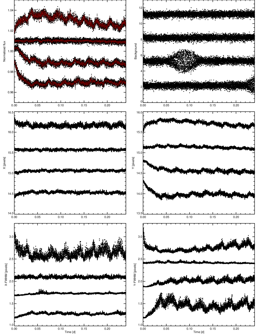
We apply the same reduction procedure for all AORs. We first convert fluxes from the Spitzer units of specific intensity (MJy/sr) to photon counts. We then perform aperture photometry on each subarray image using the APER routine from the IDL Astronomy User’s Library333http://idlastro.gsfc.nasa.gov/contents.html. We compute the stellar fluxes in aperture radii ranging between 2.0 and 4.0 pixels, the best results being obtained with an aperture radius of 3 pixels for the first and fourth AOR, 2.8 pixels for the second AOR and 2.9 pixels for the third AOR. We use background annuli extending from 11 to 15.5 pixels from the PRF center. The center and full width at half maximum (FWHM, along and axes) of the PRF is measured by fitting a Gaussian profile on each image using the MPCURVEFIT procedure (Markwardt, 2009).
Examination of the background time-series reveals an “explosion” of the flux in the third and fourth AORs, with a similar shape to the one observed in D11. These two background “explosions” seem to be correlated with an increase of the measured FWHM along the -axis. Because of the “pixel-phase” effect, changes in the PRF’s shape create an additional correlated noise contribution (Gillon et al., in prep.).
For each block of 64 subarray images, we discard the discrepant values for the measurements of flux, background, - positions and FWHM using a 10- median clipping for the six parameters. We then average the resulting values, the photometric errors being taken as the uncertainties on the average flux measurements. At this stage, a 50- clipping moving average is used on the resulting light curve to discard totally discrepant subarray-averaged fluxes. The number of frames kept for each AOR are shown in Table 1.
Figure 1 shows the raw lightcurve, the background flux, the - centroid positions and FWHM for each AOR. The improved stability of the telescope pointing achieved by the new PCRS peak-up mode can be easily noticed for the time-series but seems less sharp along the pixel’s axis.
3. Data Analysis
3.1. Independent analysis of each AOR
The aim of this step is to perform an exhaustive model comparison to determine the optimal baseline model for each AOR. The baseline model accounts for the time- and position- dependent systematic effects relevant to the IRAC-4.5 m observations (see D11, G12 and references therein). For this purpose, we individually analyze each AOR by employing our adaptative Markov-Chain Monte Carlo (MCMC) implementation described in Gillon et al. (2010). We set the occultation depth as a jump parameter and fix the orbital period , transit duration , time of minimum light and impact parameter to the values obtained from the global analysis of the system (G12). We further impose a Gaussian prior on the orbital eccentricity (, D11), allowing the eclipse phase and duration to float in the MCMC. For each model, we run two chains of steps each. Throughout this work, we assess the convergence and good mixing of the Markov chains using the statistical test from Gelman & Rubin (1992).
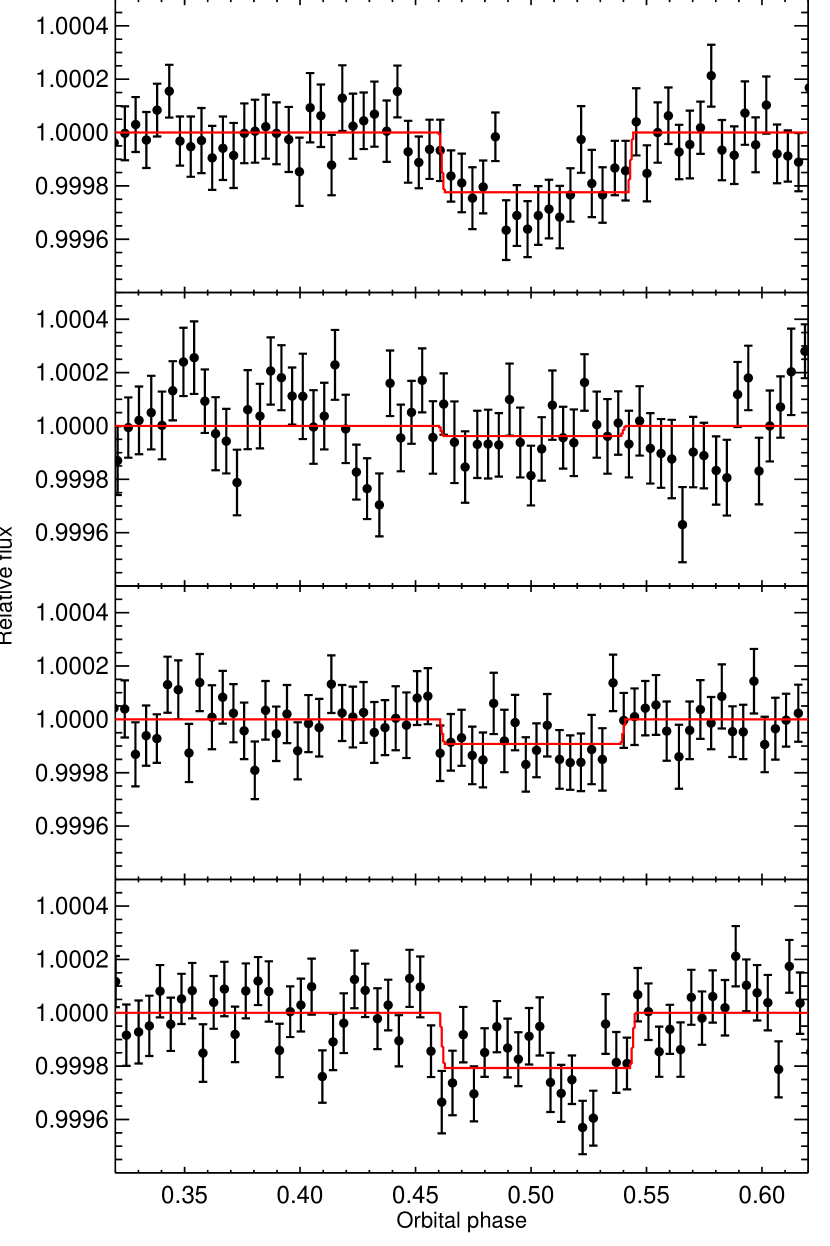
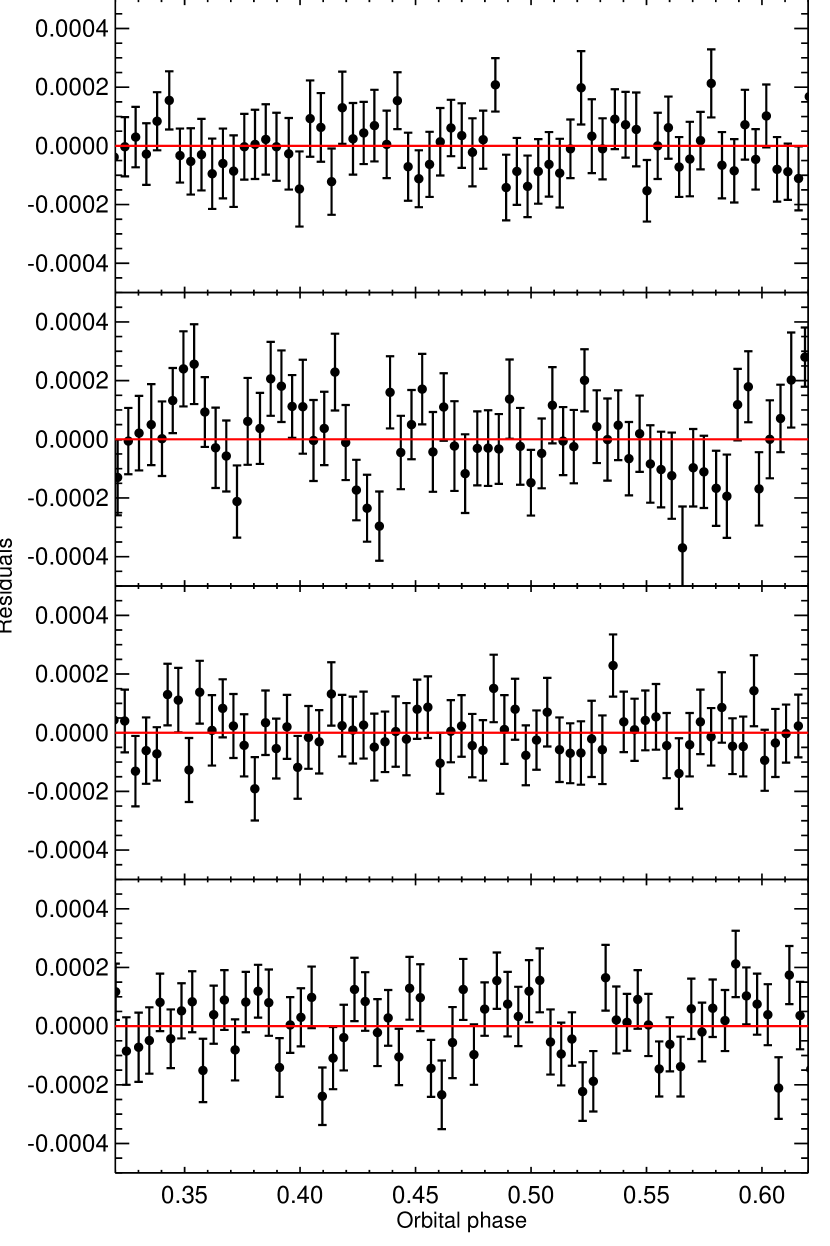
We first assume a baseline model based on a classical second order - position polynomial (D11, eq. 1) to correct the “pixel-phase” effect, added to a time-dependent linear trend. We then increase this basic baseline complexity by trying combinations of up to third- and fourth-order - position polynomials, second-order logarithmic ramp models and second-order time-dependent polynomials. The baseline models tested are therefore characterized by 7 to 20 free parameters, well constrained by the 6200 measurements of each AOR. We finally compute the Bayesian information criterion (BIC, e.g., Gelman et al., 2003) for all combinations and choose, from the MCMC output, the baseline model that yields the highest marginal likelihood. We show the resulting individual lightcurves on Fig. 2 and the selected model along with the occultation depth for each AOR in Table 1.
The correlated noise affecting each lightcurve is taken into account following Gillon et al. (2010). A scaling factor from the comparison of the standard deviation of binned and unbinned flux residuals is determined during a preliminary MCMC run. This factor is then applied to the individual uncertainties of the flux time-series. The values for each AOR are shown in Table 1. To obtain an additional estimation of the residual correlated noise, we conduct a residual-permutation bootstrap analysis on each lightcurve corrected from the baseline model, similar to D11. This part of the analysis yields parameters in good agreement with the results from our MCMC analyses, albeit with significantly smaller error bars, suggesting that the error budget is dominated by the uncertainties on the coefficients of the complex baseline model and not by the residual correlated noise contribution.
The examination of the individual lightcurves obtained with more complex models lead to similar results to the lightcurves shown on Fig. 2, that are obtained with the baseline models selected in the previous step (Table 1). The resulting occultation depths are compatible within 1, securing both our detection and the insensitivity of the occultation signal to our adopted method for systematics correction.
As in D11 and G12, we perform a Lomb-Scargle periodogram analysis (Scargle, 1982) on the residuals of our selected model for each AOR. Peaks with marginal significance are found at 69 min in the second AOR and at 51 min in the third AOR, while neither of the first nor fourth AOR’s residuals reveal a periodic signal. We include these sinusoidal modulations in the baseline models of our second and third AOR and perform a new MCMC that yields a higher BIC value than our model selected during the previous step of the analysis. We therefore neglect the sinusoidal term in both AORs. No hint of a min and ppm amplitude modulation similar to the one reported in D11 and G12 is found in the four datasets.
We further build a “pixel map” to characterize the intrapixel variability on a fine grid. This approach has been already demonstrated by Ballard et al. (2010) and Stevenson et al. (2011) as an efficient method to remove the flux modulation due to the “pixel-phase” effect. The improved tracking accuracy brought by the new PCRS peak-up mode is indeed expected to increase the resolution of the pixel map, hence motivating this step of the analysis for our observations. More specifically, our implementation divides the area covered by the PRF in a grid made of 3030 boxes and counts the number of out-of-eclipse datapoints that fall in a each box. If a given box has at least four datapoints spanning at least 50% of the AOR duration, the individual fluxes are divided by their mean, otherwise the corresponding measurements are rejected. As this method could average out an eclipse signal located in the designated out-of-eclipse parts of the lightcurve, we repeat this procedure by gradually shifting the out-of-eclipse datapoints in time. On average, as compared to the first AOR (obtained without the PCRS peak-up mode), the measurements sample 24% more time per box in the second AOR, 57% in the third AOR and 48% in the fourth AOR. The occultation depth and duration obtained using the pixel-map corrected lightcurves are in good agreement with the ones employing a polynomial baseline model.
The different analysis techniques applied above yield detrended time-series in which the occultation signal is visible by eye with consistent phase and duration in three out of the four AORs (Fig. 2). The second AOR is the only one in which the detection is marginal ( ppm). The different approaches used to correct the photometry from the “pixel-phase” effect show that the intrapixel sensitivity does not explain this discrepancy. We notice that the factor for this second AOR is 50% larger than for the other AORs (see Table 1), suggesting a larger amount of correlated noise of instrumental or astrophysical origin. Examination of the onboard temperature sensors readings and other external parameters in the FITS files do not reveal any unusual patterns. While an actual variability of the planet’s emission cannot be ruled out, the marginal disagreement (1.2) of the second occultation’s amplitude relative to the three others is probably caused by this larger correlated noise.
| AOR 1 | AOR 2 | AOR 3 | AOR 4 | GLOBAL (prior on ) | GLOBAL ( fixed) | |
|---|---|---|---|---|---|---|
| Observation date [UT] | 2012-01-18 | 2012-01-21 | 2012-01-23 | 2012-01-31 | — | — |
| Observation window [UT] | 02:45 - 08:38 | 01:16 - 07:09 | 06:24 - 12:17 | 08:56 - 14:49 | — | — |
| Number of measurements | 6187 | 6190 | 6133 | 6164 | — | — |
| Baseline modelaaBaseline models are described by position (), time () and ramp () terms, with the order indicated in superscript. | — | — | ||||
| factorbbSee Section 3 for details on the scaling factor. | 1.25 | 1.89 | 1.20 | 1.27 | — | — |
| Occultation depth [ppm] | ||||||
| — | ||||||
| — |
3.2. Global analysis
The final step of our analysis consists of performing a global analysis, including all four lightcurves in the same MCMC framework, to constrain both the occultation depth and orbital eccentricity. For this purpose, we assume Gaussian priors on , , , , and the stellar parameters based on the posterior distributions derived in D11, G12 and in von Braun et al. (2011). We first run two MCMC (one with the occultation model and one without) to assess the robustness of our detection, using as input the four raw lightcurves. We employ the baseline models selected in the previous step and shown in Table 1. These two runs are composed of three chains of steps each.
We find an occultation depth of ppm, and an eccentricity (3- upper limit). The odds ratio computed using the BIC between the two models (with vs. without occultation) is in favor of the occultation model. The thermal emission from 55 Cnc e is therefore firmly detected.
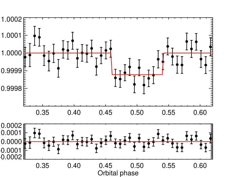
To test the robustness of the eccentricity signal, we then perform an identical MCMC run but with the assumption of a circular orbit. The odds ratio between the circular and non-circular orbits is in favor of the circular case. The resulting occultation depth in this case is ppm, in excellent agreement with the value obtained for the non-circular case. The phase-folded occultation lightcurve with the best-fit circular model is shown on Figure 3.
4. Results and Discussion
4.1. Planetary Properties
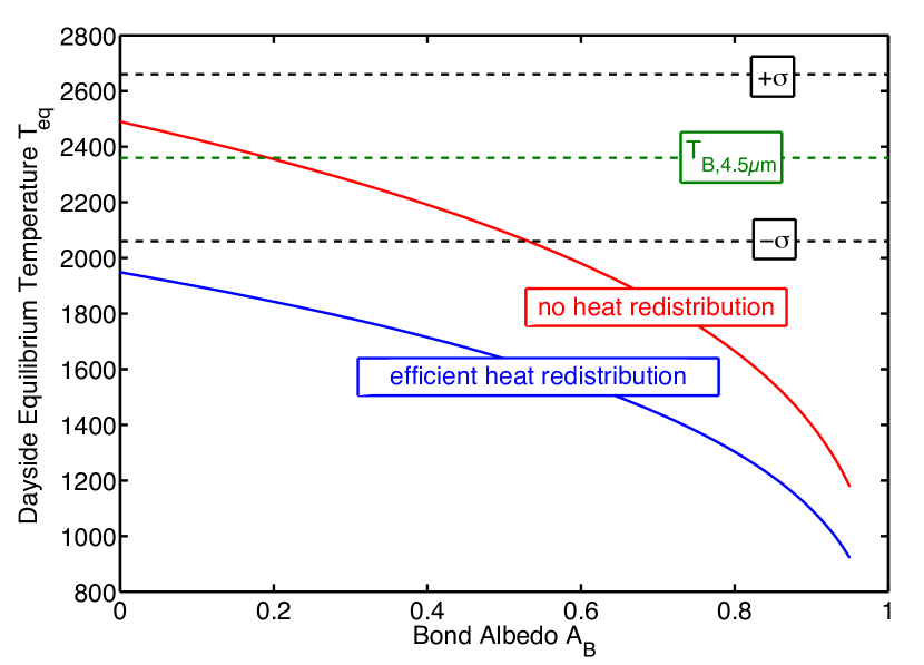
From the measured secondary eclipse depth we obtain a brightness temperature estimate of K, using a stellar blackbody emission spectrum, with K (von Braun et al., 2011). At face value, the high brightness temperature suggests that either 55 Cnc e has both a low Bond albedo and an inefficient heat transportation from the day side to the night side, or the observations in the IRAC bandpass probe layers in the atmosphere that are at temperatures higher than the equilibrium temperature (Figure 4). Either scenario may explain why the brightness temperature is observed to be higher than the zero Bond albedo equilibrium temperature, K, for a uniformly re-radiating planet.
One interpretation could be that the planet is a rock with only a minimal atmosphere established through vaporization (Schaefer & Fegley, 2009; Léger et al., 2009; Castan & Menou, 2011). Rocky objects in the Solar System, e.g., Mercury and the Moon, have low Bond albedos between 0.07 and 0.12. Lacking a thick atmosphere, a rocky super-Earth also does not have any efficient mean of transporting heat from the day-side to the night-side. We disfavor the bare rock scenario, however, because the 55 Cnc e mass and radius measurements (D11, G12) exclude a rocky composition similar to Mercury and Earth; to be a rocky planet with minimal atmosphere 55 Cnc e would have to have the unlikely bulk composition of pure silicate.
Alternatively, if 55 Cnc e has a substantial gas atmosphere or envelope, the scenario of inefficient heat redistribution is still supported by the K brightness temperature, as long as the radiation at 4.5 m is not coming from a very hot layer, such as a deep layer or a thermal inversion layer. The interpretation of 55 Cnc e having a supercritical water envelope above a solid nucleus (D11) fits with the inferred high temperature; the absence of clouds at such a high temperature results in a water envelope with a naturally low albedo. Although we cannot fully exclude the case of heat redistribution, for the water planet or even a gas atmosphere over a rocky core, the probe to deep hot layers or the thermal inversion would have to be extreme. A probe of extremely deep, hot atmosphere layers is unlikely because many of the gases likely to be present in the atmosphere, in particular and CO, have high absorption cross sections in the spectral region of the IRAC bandpass between 4 and 5 m. A thermal inversion, while present in Solar System planet atmospheres and suggested to be present in many similarly highly-irradiated hot Jupiters (e.g., Burrows et al., 2007; Knutson et al., 2008), is also an extreme explanation because the temperature would have to be K above most of the rest of the atmosphere. In general, while we know the total amount of energy re-radiated by the planet, it is the interplay between absorption of stellar radiation at short wavelength, the opacities at wavelengths at which the bulk radiation is emitted (1-5 m for a body at T K), and the opacity in our IRAC 4.5 m bandpass that sets the observed brightness temperature.
Considering the observational uncertainty, the observed brightness temperature in the IRAC bandpass could be as low as K at the 2- level. At this level of uncertainty, we can say that at least one or more of the following statements are true: 1) the planet’s Bond albedo is low; 2) the planet has an inefficient heat transport from the day to night side; and/or 3) the IRAC 4.5 m bandpass probes at atmospheric levels that are considerably hotter than the day-side equilibrium temperature.
4.2. Orbital Eccentricity
Our global MCMC analysis improves the 3- upper limit on 55 Cnc e’s orbital eccentricity from 0.25 (D11) to 0.06. However, even such a small eccentricity is unlikely because tidal interactions between the planet and star would probably damp an initial eccentricity that large in a few Myrs. Much larger initial eccentricities would be damped on similar timescales. However, high order dynamical interactions among the planets in the system may maintain an eccentricity for 55 Cnc e of a few parts per million, by comparison with theoretical studies of multi-planet systems having close-in super-Earths (Barnes et al., 2010). Strong observational constraints on 55 Cnc e’s eccentricity may even provide information about the planet’s tidal response and internal structure (Batygin et al., 2009). While a small eccentricity might have little direct influence on observation, the concomitant tidal dissipation within the planet can have dramatic geophysical consequences, perhaps powering vigorous volcanism and resupplying the planet s atmosphere (Jackson et al., 2008). The planet’s proximity to its host star suggests, in fact, it may be shedding its atmosphere, and so active resupply may be necessary for long-term atmospheric retention.
4.3. Future prospects
From the first, landmark detection of infrared light from a hot Jupiter (Charbonneau et al., 2005; Deming et al., 2005) and further occultation observations of more than two-dozen Neptune- and Jupiter-sized planets (see, e.g., Deming & Seager, 2009), Spitzer remains today the best instrument for exoplanet high-precision near-infrared photometry. At the dawn of the super-Earth sized planet discovery era (see, e.g., Batalha et al., 2012), Spitzer’s continued legacy shows the need for keeping this observatory operational. With the future launch of the James Webb Space Telescope, the exoplanet community anticipates thermal emissions measurements for a number of different super Earths (see, e.g., Deming et al., 2009), hence improving our knowledge of this class of planets in a way similar to the achievements made by Spitzer for hot Jupiters.
References
- Ballard et al. (2010) Ballard, S., Charbonneau, D., Deming, D., et al. 2010, PASP, 122, 1341
- Barnes et al. (2010) Barnes, R., Raymond, S. N., Greenberg, R., Jackson, B., & Kaib, N. A. 2010, ApJ, 709, L95
- Batalha et al. (2012) Batalha, N. M., Rowe, J. F., Bryson, S. T., et al. 2012, ArXiv e-prints
- Batygin et al. (2009) Batygin, K., Bodenheimer, P., & Laughlin, G. 2009, ApJ, 704, L49
- Burrows et al. (2007) Burrows, A., Hubeny, I., Budaj, J., Knutson, H. A., & Charbonneau, D. 2007, ApJ, 668, L171
- Butler et al. (1997) Butler, R. P., Marcy, G. W., Williams, E., Hauser, H., & Shirts, P. 1997, Astrophysical Journal Letters v.474, 474, L115
- Castan & Menou (2011) Castan, T., & Menou, K. 2011, ApJ, 743, L36
- Charbonneau (2003) Charbonneau, D. 2003, Scientific Frontiers in Research on Extrasolar Planets, 294, 449
- Charbonneau et al. (2005) Charbonneau, D., Allen, L. E., Megeath, S. T., et al. 2005, ApJ, 626, 523
- Cowan & Agol (2011) Cowan, N. B., & Agol, E. 2011, ApJ, 729, 54
- Dawson & Fabrycky (2010) Dawson, R. I., & Fabrycky, D. C. 2010, ApJ, 722, 937
- Deming & Seager (2009) Deming, D., & Seager, S. 2009, Nature, 462, 301
- Deming et al. (2005) Deming, D., Seager, S., Richardson, L. J., & Harrington, J. 2005, Nature, 434, 740
- Deming et al. (2009) Deming, D., Seager, S., Winn, J., et al. 2009, PASP, 121, 952
- Demory et al. (2011) Demory, B.-O., Gillon, M., Deming, D., et al. 2011, A&A, 533, 114
- Fazio et al. (2004) Fazio, G. G., Hora, J. L., Allen, L. E., et al. 2004, ApJS, 154, 10
- Fischer et al. (2008) Fischer, D. A., Marcy, G. W., Butler, R. P., et al. 2008, ApJ, 675, 790
- Gelman & Rubin (1992) Gelman, & Rubin. 1992, Statistical Science, 7, 457
- Gelman et al. (2003) Gelman, A., Carlin, J. B., Stern, H. S., & Rubin, D. B. 2003, Bayesian Data Analysis, Second Edition (Chapman & Hall/CRC Texts in Statistical Science), 2nd edn. (Chapman and Hall/CRC)
- Gillon et al. (2010) Gillon, M., Lanotte, A. A., Barman, T., et al. 2010, A&A, 511, 3
- Gillon et al. (2012) Gillon, M., Demory, B.-O., Benneke, B., et al. 2012, A&A, 539, A28
- Jackson et al. (2008) Jackson, B., Barnes, R., & Greenberg, R. 2008, MNRAS, 391, 237
- Knutson et al. (2008) Knutson, H. A., Charbonneau, D., Allen, L. E., Burrows, A., & Megeath, S. T. 2008, ApJ, 673, 526
- Léger et al. (2009) Léger, A., Rouan, D., Schneider, J., et al. 2009, A&A, 506, 287
- Marcy et al. (2002) Marcy, G. W., Butler, R. P., Fischer, D. A., et al. 2002, ApJ, 581, 1375
- Markwardt (2009) Markwardt, C. B. 2009, Astronomical Data Analysis Software and Systems XVIII ASP Conference Series, 411, 251
- McArthur et al. (2004) McArthur, B. E., Endl, M., Cochran, W. D., et al. 2004, ApJ, 614, L81
- Scargle (1982) Scargle, J. D. 1982, ApJ, 263, 835
- Schaefer & Fegley (2009) Schaefer, L., & Fegley, B. 2009, ApJ, 703, L113
- Stevenson et al. (2011) Stevenson, K. B., Harrington, J., Fortney, J., et al. 2011, ArXiv e-prints
- von Braun et al. (2011) von Braun, K., Boyajian, T. S., ten Brummelaar, T. A., et al. 2011, ApJ, 740, 49
- Winn et al. (2011) Winn, J. N., Matthews, J. M., Dawson, R. I., et al. 2011, ApJ, 737, L18
- Wisdom (2005) Wisdom, J. 2005, American Astronomical Society, 36, 525