Spinor states on a curved infinite disc with non-zero spin-connection fields

Abstract

In the paper of Lukman, Mankoč Borštnik, Nielsen (NJP 13 (2011) 103027) one step towards the realistic Kaluza-Klein[like] theories was made by presenting the case of a spinor in $d=(1+5)$ compactified on an (formally) infinite disc with the zweibein which makes a disc curved on an almost $S^{2}$ and with the spin connection field which allows on such a sphere only one massless spinor state of a particular charge, coupling the spinor chirally to the corresponding Kaluza-Klein gauge field. The solutions for the massless spinor state were found for a range of spin connection fields, as well as the massive ones for a particular choice of the spin connection field. In this paper we present the massless and massive spinor states for the whole range of parameters of the spin connection field which allow only one massless solution.

Keywords: Unifying theories, Kaluza-Klein theories, mass protection mechanism, higher dimensional spaces, solutions of Dirac equations, solutions of second order differential equations

1 Introduction

This paper is the continuation of the paper entitled ”An effective two dimensionality” cases bring a new hope to the Kaluza-Klein[like] theories [1], in which the authors (the third one is H.B. Nielsen) proved on a toy model that when the space breaks from $M^{1+(d-1)}$ to $M^{1+3}\times$ a non compact space there can exist in $M^{1+3}$ a massless solution for a spinor, chirally coupled to the corresponding Kaluza-Klein field, if the spin connection field and the vielbein on a non compact space are properly chosen  . Although we did just assume the two fields used (not showed how they are generated, say, due to the presence of some spinor fields in interaction with some vielbeins and spin connections not mentioned in the paper) yet we succeeded to find the analytical solutions for a massless spinor for the whole allowed interval of the parameter of the (chosen) spin connection field and the spectrum for massive solutions for a particular choice of the parameter.

In this paper we present the masses and states for spinors living on $M^{1+3}\times$ an almost $S^{2}$ sphere on which the parameter of the chosen spin connection field is allowed to change in the interval, which assures normalisable solutions. We prove that the presented solutions are the only normalisable ones and that they form a complete basis.

The reader, who is not willing to follow the introduction into the equations of motion for the two unknown functions $\mathcal{A}_{n}$ and $\mathcal{B}_{n+1}$, which determine the spinor states on an almost $S^{2}$ sphere with a particular spin connection on it, can jump directly to the coupled equations of motion (1, 2) of the first order and further to the two differential equations of motion of the second order for the unknown functions $\mathcal{A}_{n}$ (2) and $\mathcal{B}_{n+1}$ (2), the solutions of which are interesting by themselves. (She or he might like to see which physical problem initiated the equations, at the end, if at all.) First of the two equations (2) namely simplifies, when putting the parameter ($\varepsilon$) of the spin connection field equal to $0$, to the equation for the Legendre polynomials, while solutions for the second equation (2) are expressible, when using the solutions of the first one (2) and one of the two coupled first order differential equations of motion (1), in quite an elegant way. For a general choice of the parameter ($\varepsilon$) from the allowed interval, determining the spin connection field, the solutions are expressible with the finite sum of the associate Legendre polynomials.

We shall here briefly repeat the part from the paper [1] needed to come to (1).

Let us start with the action for massless (Weyl) spinors [1] living on the manifold $M^{1+5}$

$$S = \int d^{d}x\,{\cal L}_{W}\,,$$

$${\cal L}_{W} = \frac{1}{2}[(\psi^{\dagger}E\gamma^{0}\gamma^{a}p_{0a}\psi)+(\psi^{\dagger}E\gamma^{0}\gamma^{a}p_{0a}\psi)^{\dagger}]\,,$$

$$p_{0a} = f^{\alpha}{}_{a}p_{0\alpha}+\frac{1}{2E}\,\{p_{\alpha},Ef^{\alpha}{}_{a}\}_{-}\,,$$

$$p_{0\alpha} = p_{\alpha}-\frac{1}{2}\,S^{ab}\,\omega_{ab\alpha}\,.$$ (1)

Here $f^{\alpha}{\!}_{a}$ are the vielbeins  (the gauge fields of the infinitesimal generators of translation) and $\omega_{ab\alpha}$ the spin connections (the gauge fields of $S^{ab}=\frac{i}{4}(\gamma^{a}\gamma^{b}-\gamma^{b}\gamma^{a})$). The notation $\{A,B\}_{\mp}$ means $\{AB\mp BA\}$. Correspondingly the Lagrange density for a spinor reads

$${\cal L}_{W} = \psi^{\dagger}\,\gamma^{0}\gamma^{a}E\{f^{\alpha}{}_{a}p_{\alpha}+\frac{1}{2E}\{p_{\alpha},f^{\alpha}{}_{a}E\}_{-}-\frac{1}{2}S^{cd}\omega_{cda}\}\psi.$$ (2)

Space $M^{1+5}$ has after the break the symmetry of $M^{1+3}\times$ an infinite disc with the zweibein on the disc

$$e^{s}{}_{\sigma}=f^{-1}\pmatrix{1&0\cr 0&1\cr},f^{\sigma}{}_{s}=f\pmatrix{1&0\cr 0&1\cr}\,,$$ (3)

where

$$f = 1+(\frac{\rho}{2\rho_{0}})^{2}=\frac{2}{1+\cos\vartheta}=\frac{2}{1+x}\,,$$

$$x^{(5)} = \rho\,\cos\phi,\quad x^{(6)}=\rho\,\sin\phi,\quad E=f^{-2}\,,$$

$$0\leq \phi \leq 2\pi\,,\quad 0\leq\rho\leq\infty\,,-1\leq\cos\theta\leq 1\,,$$ (4)

$$\quad x=\frac{1-(\frac{\rho}{2\rho_{0}})^{2}}{1+(\frac{\rho}{2\rho_{0}})^{2}}\,,\quad\quad-1\leq x\leq 1\,.$$

We use indices $s,t=(5,6),$ to describe the flat index in the space of an infinite plane, and $\sigma,\tau=(5),(6),$ to describe the Einstein index. With $\phi$ we denote the angle of rotations around the axis perpendicular to the disc. The angle $\vartheta$ is the ordinary azimuth angle on a sphere. The last relation follows from $ds^{2}=e_{s\sigma}e^{s}{}_{\tau}dx^{\sigma}dx^{\tau}=f^{-2}(d\rho^{2}+\rho^{2}d\phi^{2})$. Here $\rho_{0}$ is the radius of an almost $S^{2}$ sphere. The volume of this non compact sphere is finite, equal to $V=\pi\,(2\rho_{0})^{2}$. The symmetry of $S^{2}$ is a symmetry of $U(1)$ group.

There is also a spin connection field on a disc, chosen to be

$$f^{\sigma}{}_{s^{\prime}}\,\omega_{st\sigma} = iF\,f\,\varepsilon_{st}\;\frac{e_{s^{\prime}\sigma}x^{\sigma}}{(\rho_{0})^{2}}\,,\quad 0<2F\leq 1\,,\quad s=5,6,\,\,\;\sigma=(5),(6)\,.$$ (5)

It compensates in the particular case when $2F=1$ the term $\frac{1}{2E}\{p_{\sigma},f^{\sigma}{}_{s}\}_{-}$ for spinors of one of the handedness (1) and determines the spectrum of a massless and massive states to be $(m\rho_{0})^{2}=l(l+1)$, with $l=\{0,1,2,\cdots\}$.

We require normalizability (needed like in any of this kind of problems to lead to operative solutions) of states $\psi$ on the disc

$$\int_{0}^{2\pi}\,d\phi\;\int_{0}^{\infty}\;\rho d\rho\psi^{\dagger}\psi<\infty.$$ (6)

We assume to have no gravity in $d=(1+3)$ ($f^{\mu}{}_{m}=\delta^{\mu}_{m}$ and $\omega_{mn\mu}=0$ for $m,n=0,1,2,3,\ldots;\;,\mu=0,1,2,3,\ldots$).

It is proven in [1] that there are chiral fermions on this almost sphere with the spin connection field on it without including any extra fundamental gauge fields: A massless spinor of only one handedness, and correspondingly mass protected, which couples to the corresponding Kaluza-Klein fields.

The equations of motion for spinors (the Weyl equations), which follow from the Lagrange density (2) when assuming that there is no gravity in $d=(1+3)$, are then

$$\{E\gamma^{0}\gamma^{m}p_{m}+Ef\gamma^{0}\gamma^{s}\delta^{\sigma}_{s}(p_{0\sigma}+\frac{1}{2Ef}\{p_{\sigma},Ef\}_{-})\}\psi=0,\quad{\rm with}$$

$$p_{0\sigma}=p_{\sigma}-\frac{1}{2}S^{st}\omega_{st\sigma}\,,$$ (7)

with $f$ from (1) and with $\omega_{st\sigma}$ from (5). Let us add that the vielbein curling the disc into an almost $S^{2}$ does not break the rotational symmetry on the disc, it breaks the translation symmetry after making a choice of the northern and southern pole.

The solution of the equations of motion (7) for a spinor in $(1+5)$-dimensional space, which breaks into $M^{(1+3)}$ and a non compact $S^{2}$, is a superposition of all four ($=2^{6/2-1}$) states of a single Weyl representation. (We kindly ask the reader to see the technical details about how to write a Weyl representation in terms of the Clifford algebra objects after making a choice of the Cartan subalgebra, for which we take $S^{03},S^{12}$ and $S^{56}$, in [1, 15].) In our technique one spinor representation—the four states, which all are the eigen states of the chosen Cartan subalgebra with the eigen values $\frac{k}{2}$—are the following four products of projectors $\stackrel{{\scriptstyle ab}}{{[k]}}$ and nilpotents $\stackrel{{\scriptstyle ab}}{{(k)}}$:

$$\varphi^{1}_{1} = \stackrel{{\scriptstyle 56}}{{(+)}}\stackrel{{\scriptstyle 03}}{{(+i)}}\stackrel{{\scriptstyle 12}}{{(+)}}\psi_{0}\,,$$

$$\varphi^{1}_{2} = \stackrel{{\scriptstyle 56}}{{(+)}}\stackrel{{\scriptstyle 03}}{{[-i]}}\stackrel{{\scriptstyle 12}}{{[-]}}\psi_{0}\,,$$

$$\varphi^{2}_{1} = \stackrel{{\scriptstyle 56}}{{[-]}}\stackrel{{\scriptstyle 03}}{{[-i]}}\stackrel{{\scriptstyle 12}}{{(+)}}\psi_{0}\,,$$

$$\varphi^{2}_{2} = \stackrel{{\scriptstyle 56}}{{[-]}}\stackrel{{\scriptstyle 03}}{{(+i)}}\stackrel{{\scriptstyle 12}}{{[-]}}\psi_{0}\,,$$ (8)

where $\psi_{0}$ is a vacuum state for the spinor state. The most general wave function $\psi^{(6)}$ obeying (7) in $d=(1+5)$ can now be written as

$$\psi^{(6)}={\cal A}\,{\stackrel{{\scriptstyle 56}}{{(+)}}}\,\psi^{(4)}_{(+)}+{\cal B}\,{\stackrel{{\scriptstyle 56}}{{[-]}}}\,\psi^{(4)}_{(-)}\,.$$ (9)

${\cal A}$ and ${\cal B}$ depend on $x^{\sigma}$ and $\psi^{(4)}_{(+)}$ and $\psi^{(4)}_{(-)}$ determine the spin and the coordinate dependent parts of the wave function $\psi^{(6)}$ in $d=(1+3)$

$$\psi^{(4)}_{(+)} = \alpha_{+}\;{\stackrel{{\scriptstyle 03}}{{(+i)}}}\,{\stackrel{{\scriptstyle 12}}{{(+)}}}+\beta_{+}\;{\stackrel{{\scriptstyle 03}}{{[-i]}}}\,{\stackrel{{\scriptstyle 12}}{{[-]}}}\,,$$

$$\psi^{(4)}_{(-)} = \alpha_{-}\;{\stackrel{{\scriptstyle 03}}{{[-i]}}}\,{\stackrel{{\scriptstyle 12}}{{(+)}}}+\beta_{-}\;{\stackrel{{\scriptstyle 03}}{{(+i)}}}\,{\stackrel{{\scriptstyle 12}}{{[-]}}}\,.$$ (10)

If one uses $\psi^{(6)}$ of (9) in (7), separates dynamics in $(1+3)$ and on $S^{2}$, expresses $x^{(5)}$ and $x^{(6)}$ from (1) and takes the zweibein from (3, 1) and the spin connection from (5), the equation (7) transforms as follows

$$if\,\{e^{i\phi 2S^{56}}\,[\frac{\partial}{\partial\rho}+\frac{i\,2S^{56}}{\rho}\,(\frac{\partial}{\partial\phi})-\frac{1}{2\,f}\,\frac{\partial f}{\partial\rho}\,(1-2F\,2S^{56})\,]\,\}\,\psi^{(6)}+\gamma^{0}\gamma^{5}\,m\,\psi^{(6)}=0\,.$$ (11)

$\psi^{(6)}$ can be chosen to be the eigen function of the total angular momentum $M^{56}=-i\frac{\partial}{\partial\phi}+S^{56}$

$$\psi^{(6)}={\cal N}_{n}\,({\cal A}_{n}\,\stackrel{{\scriptstyle 56}}{{(+)}}\,\psi^{(4)}_{(+)}+{\cal B}_{n+1}\,e^{i\phi}\,\stackrel{{\scriptstyle 56}}{{[-]}}\,\psi^{(4)}_{(-)})\,e^{in\phi}\,,$$ (12)

with the property

$$M^{56}\psi^{(6)}=(n+\frac{1}{2})\,\psi^{(6)}\,.$$ (13)

Here ${\cal N}_{n}$ is the normalization constant. Taking into account that $S^{56}\stackrel{{\scriptstyle 56}}{{(+)}}=\frac{1}{2}\stackrel{{\scriptstyle 56}}{{(+)}}$, and $S^{56}\stackrel{{\scriptstyle 56}}{{[-]}}=-\frac{1}{2}\stackrel{{\scriptstyle 56}}{{[-]}}$, and introducing the coordinate $x$ from (1) instead of $\rho$, we end up with the equations of motion for ${\cal A}_{n}$ and ${\cal B}_{n+1}$ as follows

$$-i\left[-\sqrt{1-x^{2}}\left(\frac{d}{dx}-\frac{n+1}{1-x^{2}}\right)-\frac{1+2F}{2}\sqrt{\frac{1-x}{1+x}}\right]\mathcal{B}_{n+1}+m\rho_{0}\mathcal{A}_{n}=0\,,$$

$$-i\left[-\sqrt{1-x^{2}}\left(\frac{d}{dx}+\frac{n}{1-x^{2}}\right)-\frac{1-2F}{2}\sqrt{\frac{1-x}{1+x}}\right]\mathcal{A}_{n}+m\rho_{0}\mathcal{B}_{n+1}=0\,,$$

$$-1\leq x\leq 1\,,\quad 0\leq(1-2F)<1\,.$$ (14)

The interval of the coordinate $x$, $(-1\leq x\leq 1)$, corresponds to the interval of the coordinate $\rho$, $(0\leq\rho\leq\infty)$. The spinor part ($\stackrel{{\scriptstyle 56}}{{(+)}}$, $\stackrel{{\scriptstyle 56}}{{[-]}}$) and the angular part $e^{in\phi}$, both manifest orthogonality.

For any $F$ within the interval $0<2F\leq 1$ only one normalisable massless spinor state on $S^{2}$ exists [1]. In the particular case that $2F=1$ the spin connection term $-S^{56}\omega_{56\sigma}$ compensates the term $\frac{1}{2Ef}\{p_{\sigma},Ef\}_{-}$ for the left handed spinor with respect to $d=1+3$, while for the spinor of the opposite handedness, again with respect to $d=1+3$, the spin connection term doubles the term $\frac{1}{2Ef}\{p_{\sigma},Ef\}_{-}$: The term $\sqrt{\frac{1-x}{1+x}}$ in (1) is multiplied by $1$ in the first equation and by $0$ in the second equation.

While the massless solution was found in [1] for the whole interval of the parameter $F$, $(0\leq(1-2F)<1)$, the massive spectrum was presented only for the particular case $2F=1$.

In this paper we find the spectrum for the whole interval of $F$, $(0\leq(1-2F)<1)$.

2 Solutions of the equations of motion for spinors

We look in this section for the spectrum of the equation of motion (1) for an arbitrary choice of the parameter $F$ within the interval $0<2F\leq 1$. We allow only normalisable solutions (9, 12). Taking into account that $E\rho d\rho=dx$ it follows for the normalizability requirement

$$2\pi\,\int^{1}_{-1}\,dx\,{\cal A}^{\star}_{n}{\cal A}_{n} <\infty\,,$$

$$2\pi\,\int^{1}_{-1}\,dx\,{\cal B}^{\star}_{n}{\cal B}_{n} <\infty\,.$$ (15)

Let us, for simplicity, introduce a new parameter $2F=1-2\varepsilon$ and rewrite (1) with this new parameter $\varepsilon$

$$-i\left[-\sqrt{1-x^{2}}\left(\frac{d}{dx}-\frac{n+1}{1-x^{2}}\right)-(1-\varepsilon)\sqrt{\frac{1-x}{1+x}}\right]\mathcal{B}_{n+1}+m\rho_{0}\mathcal{A}_{n}=0,$$

$$-i\left[-\sqrt{1-x^{2}}\left(\frac{d}{dx}+\frac{n}{1-x^{2}}\right)-\varepsilon\sqrt{\frac{1-x}{1+x}}\right]\mathcal{A}_{n}+m\rho_{0}\,\mathcal{B}_{n+1}=0,\,$$

$$0\leq\varepsilon<\frac{1}{2}\,.$$ (16)

One easily finds the massless ($m\,\rho_{0}=0$) normalisable solutions [1] for $\mathcal{A}_{n}$ for any $0\leq\varepsilon<\frac{1}{2}$ ($0<2F\leq 1$)

$$\mathcal{A}_{n}=\mathcal{A}_{o}\,\rho^{n}f^{\varepsilon}=\mathcal{A}_{o}\,(1-x)^{\frac{n}{2}}(1+x)^{-\frac{n}{2}-\varepsilon}\,\rho_{0}^{n}\,2^{n+\varepsilon}.$$ (17)

The corresponding massless solution for $\mathcal{B}_{n}$

$$\mathcal{B}_{n}=\mathcal{B}_{o}\,\rho^{-n}f^{1-\varepsilon}=\mathcal{B}_{o}\,(1-x)^{-\frac{n}{2}}(1+x)^{\frac{n}{2}+\varepsilon-1}\,2^{-n+1-\varepsilon}\,\rho_{0}^{-n}$$ (18)

is not normalisable. The normalisation condition namely requires [1]

$${\rm for}\;{\cal A}_{n}:\,-1<n<(1-2\varepsilon)\,,$$

$${\rm for}\;{\cal B}_{n}:(1-2\varepsilon)<n<1,\quad n\;\;{\rm is\;\;an\;\;integer}\,.$$ (19)

For $(0\leq\varepsilon<\frac{1}{2})$ one immediately sees that this is for an integer $n$ possible only for $n=0$, ${\cal A}_{n}={\cal A}_{0}$ (17) and ${\cal B}_{n}=0$ (18).

Equation (19) tells us that the strength $F$ ($=(\frac{1}{2}-\varepsilon$)) of the spin connection field $\omega_{56\sigma}$ makes a choice between the two massless solutions ${\cal A}_{0}$ and ${\cal B}_{0}$.

To look for massive solutions of (2) we express the eigen states in terms of the associate Legendre polynomials $P^{l}_{n}$, which solve the equation

$$\{(1-x^{2})\frac{d^{2}}{dx^{2}}-2x\frac{d}{dx}+(l(l+1)-\frac{n^{2}}{1-x^{2}})\}P^{l}_{n}=0\,.$$ (20)

One can prove that the Legendre polynomials form a normalisable

$$\int_{-1}^{1}\,P^{l}_{n}\,P^{l^{\prime}}_{n}\,dx = \frac{2}{2l+1}\,\frac{(l+n)!}{(l-n)!}\,\delta_{ll^{\prime}}\,,$$

$$\int_{-1}^{1}\,P^{l}_{n}\,P^{l}_{n^{\prime}}\,\frac{dx}{1-x^{2}} = \frac{1}{n}\,\frac{(l+n)!}{(l-n)!}\,\delta_{nn^{\prime}}\,,$$

$$l,l^{\prime}\geq n\,;\quad n,n^{\prime}\geq 0\,,$$ (21)

and complete set [17, 18, 1] in the interval $-1\leq x\leq 1$ only for an integer $l$ ($P^{\lambda}_{\nu}$ is not square integrable for $\lambda$ not an integer $l$) and an integer $n$ ($P^{\lambda}_{\nu}$ is not square integrable for $\nu$ not an integer $n$). Due to the orthogonality of the spinor and angular parts by themselves in (12) we need only the orthogonality relation of the first line in (2).

Let us transform (2), which are the two coupled first order equations, into the two second order equations for $\mathcal{A}_{n}$ and $\mathcal{B}_{n+1}$

$$(1-x^{2})\frac{d^{2}}{dx^{2}}\mathcal{A}_{n}-2x\frac{d}{dx}\mathcal{A}_{n}+(m\rho_{0})^{2}\mathcal{A}_{n}$$

$$-\left\{\frac{n^{2}}{1-x^{2}}+\frac{1}{1+x}\varepsilon(1+x+2n)+\varepsilon^{2}\frac{1-x}{1+x}\right\}\mathcal{A}_{n}=0\,,$$ (22)

$$(1-x^{2})\frac{d^{2}}{dx^{2}}\mathcal{B}_{n+1}-2x\frac{d}{dx}\mathcal{B}_{n+1}+(m\rho_{0})^{2}\mathcal{B}_{n+1}$$

$$+\left\{-\frac{(n+1)^{2}}{1-x^{2}}+\frac{2n(1-\varepsilon)}{1+x}+\varepsilon(1-\varepsilon)\frac{1-x}{1+x}\right\}\mathcal{B}_{n+1}=0\,.$$ (23)

We immediately see that for $\varepsilon=0$ the normalisable solutions of (2) are the associate Legendre polynomials ${\cal A}^{l}_{n}=P^{l}_{n}$ of (20) and that the mass spectrum must be discrete, $(m\rho_{0})^{2}=l(l+1)$, ($l=\{0,1,2,\cdots\}$), in order that the solutions fulfil the normalisability condition of (15). The solutions ${\cal B}^{l}_{n}$ of (2) follow from the second equation of (2) once ${\cal A}^{l}_{n}$ are known.

To find the normalisable solutions of (2, 2) for any $\varepsilon$ in the interval $0\leq\varepsilon<\frac{1}{2}\,$ one could expand solutions in terms of $P^{l}_{n}$, ${\cal A}_{n}=\sum_{l=n,\infty}\,\alpha^{l}_{n}\,P^{l}_{n}$ and ${\cal B}_{n}=\sum_{l=n,\infty}\,\beta^{l}_{n}\,P^{l}_{n}$. The recurrence relations for the coefficients $\alpha^{l}_{n}$ and $\beta^{l}_{n}$, which follow when using these two expansion in (2, 2) and taking into account (20), are presented in C (equations (C, C)). It is, however, very difficult to see when using these two expansions in terms of the Legendre polynomials for which values of the mass term $m\rho_{0}$ are solutions normalisable.

It is much more convenient to find a normalisable and useful ansatz by evaluating the behaviour of solutions of (2, 2) at $x\to 1$ and at $x\to-1$. This is done in subsect. 2.1. We find for ${\cal A}_{n}$ and $0\leq\varepsilon<\frac{1}{2}$

$$\mathcal{A}_{n} = (1+x)^{-\varepsilon}\,\sum_{l=n}^{\infty}\,a^{l}_{n}\,P^{l}_{n}\,.$$ (24)

For ${\cal B}_{n+1}$ and $0\leq\varepsilon<\frac{1}{2}$ we find

$$\mathcal{B}_{n+1} = (1+x)^{-\varepsilon+\frac{1}{2}}\,\sum_{l=n}^{\infty}\,b^{l}_{n}\,P^{l}_{n}\,.$$ (25)

We shall make use of (24) and use the second equation of (2) to find the solutions for $\mathcal{B}_{n+1}$.

Using this ansatz in (2), and taking into account that the first line in (2) is for each $l$ equal to ($-l(l+1)+(m\rho_{0})^{2}$), the recursion relation for the coefficients $a^{l}_{n}$ follows

$$a^{l+1}_{n}\frac{l+n+1}{2l+3}\,\left[(m\rho_{0})^{2}-(l+2)(l+1+2\varepsilon)\right]=$$

$$-a^{l}_{n}\,\left[(m\rho_{0})^{2}-l(l+1)-2n\varepsilon\right]$$

$$-a^{l-1}_{n}\frac{l-n}{2l-1}\left[(m\rho_{0})^{2}-(l-1)(l-2\varepsilon)\right].$$ (26)

Let us have a look at how does this recursive relation manifest at $l\to\infty$ for a fixed $n$ and a fixed $(m\rho_{0})^{2}$. One finds

$$a^{l+1}_{n}\,\frac{1}{2} = -a^{l}_{n}-a^{l-1}_{n}\,\frac{1}{2}\,,\quad{\rm or}$$

$$a^{l}_{n} = -\frac{a^{l+1}_{n}+a^{l-1}_{n}}{2}\,.$$ (27)

This means that coefficients $a^{l}_{n}$ are for large $l\to\infty$ up to a sign all equal. Since the Legendre polynomials $P^{l}_{n}$ are for each $n$ orthogonal, while their normalisation factor (2) is proportional to $\frac{2}{2l+1}$, and

$$\sum_{l=n}^{\infty}\,\frac{2}{2l+1}\to\infty\,,$$ (28)

this means that for the normalisable solution (24) only a finite sum over Legendre polynomials is allowed. This further means that there must be $l_{0}$, $l_{0}\geq n$, which closes the sum. Let us accordingly require for each $l\geq l_{0}$ that

$$a^{l_{0}+2}_{n}=0=a^{l_{0}+1}_{n}\,,\quad a^{l_{0}}_{n}\neq 0\,.$$ (29)

It follows from (2)

$$0=0-a^{l_{0}}_{n}\,\frac{l_{0}+1-n}{2l_{0}+1}\,[(m\rho_{0})^{2}-l_{0}(l_{0}+1-2\varepsilon)]\,,$$ (30)

which only can be fulfilled for

$$(m\rho_{0})^{2}=l_{0}(l_{0}+1-2\varepsilon)\,,$$

$$0\leq\varepsilon<\frac{1}{2}\,.$$ (31)

Equation (2) determines the mass spectrum of spinors on the infinite disc curved into an almost $S^{2}$ and with the spin connection from (5). The recursion relation in (2) determines the solution $\mathcal{A}^{l_{0}}_{n}$ for a particular $l_{0}$

$$\mathcal{A}^{l_{0}}_{n} = (1+x)^{-\varepsilon}\,\sum_{l=n}^{l_{0}}\,a^{l}_{n}\,P^{l}_{n}\,.$$ (32)

The corresponding $\mathcal{B}_{n+1}$ can be found if using the second of equations in (2) and the relations among Legendre polynomials, presented in B as

$$\mathcal{B}^{l_{0}}_{n+1}=-\frac{i\,(1+x)^{-\varepsilon}}{\sqrt{l_{0}(l_{0}+1-2\varepsilon)}\sqrt{1-x^{2})}}\,\times$$

$$\sum_{l=n}^{l_{0}}\,a^{l}_{n}\,\{n\,P^{l}_{n}+\frac{1}{(2l+1)}[(l+n)(l+1)P^{l-1}_{n}-l(l-n+1)P^{l+1}_{n}]\}\,.$$ (33)

Solutions Equation (12) can now be written as

$$\psi^{(6)l_{0}}_{n}={\cal N}^{l_{0}}_{n}\,\left({\cal A}^{l_{0}}_{n}\,\stackrel{{\scriptstyle 56}}{{(+)}}\,\psi^{(4)}_{(+)}+{\cal B}^{l_{0}}_{n+1}\,e^{i\phi}\,\stackrel{{\scriptstyle 56}}{{[-]}}\,\psi^{(4)}_{(-)}\right)\,e^{in\phi}\,,$$

$$(m\rho_{0})^{2}=l_{0}(l_{0}+1-2\,\varepsilon)\,,$$

$$0\leq\varepsilon<\frac{1}{2}\,,$$ (34)

with ${\cal A}^{l_{0}}_{n}$ from (32, 2) and ${\cal B}^{l_{0}}_{n+1}$ from (2). Since the associate Legendre polynomials form a complete normalisable set, as we pointed out when discussing the properties of solutions of (20, 2), the solutions presented in (34) form the only normalisable solutions of (2, 2).

For a special case of $\varepsilon=0$ we reproduce the spectrum presented in the ref. [1] with $(m\rho_{0})^{2}=l_{0}(l_{0}+1)$. The recursive relation (2) allows in this case only one nonzero coefficient, namely $a^{l_{0}}_{n}$, which we immediately see if putting $a^{l_{0}+1}_{n}=0$ for $\varepsilon=0$ and obtain $a^{l_{0}-1}_{n}=0.$ Consequently all the rest of coefficients are equal to zero due to (2). The solution for $\varepsilon=0$ then reads

$$\psi^{(6)l_{0}}_{n+1/2}={\cal N}^{l_{0}}_{n+1/2}\,\biggl{(}\stackrel{{\scriptstyle 56}}{{(+)}}\psi^{(4)}_{(+)}$$

$$+\frac{i}{2\sqrt{l_{0}(l_{0}+1)}}\,\stackrel{{\scriptstyle 56}}{{[-]}}\,\psi^{(4)}_{(-)}\,e^{i\phi}\,\sqrt{1-x^{2}}\,(\frac{d}{dx}\,-\frac{n}{1-x^{2}})\,\biggr{)}\cdot\,e^{in\phi}\,P^{l_{0}}_{n}\,.$$ (35)

For $l_{0}=0$ the (only) massless solution $\psi^{(6)0}_{1/2}=$ ${\cal N}^{0}_{1/2}\,\stackrel{{\scriptstyle 56}}{{(+)}}\psi^{(4)}_{(+)}$ follows.

In sect. 3 the solutions (34) are presented and their properties discussed for several choices of $\varepsilon$ in the interval $0\leq\varepsilon<\frac{1}{2}$.

2.1 Behaviour of solutions of equations of motion at $x=-1$ and $x=1$

In this section we study behaviour of solutions of (2, 2) in the vicinity of the two ends of the interval $-1\leq x\leq 1$. We find a normalisable ansatz for solutions of (2) by evaluating the contributions of $\int\,dx|{\cal A}_{n}|^{2}$ and $\int\,dx\,|{\cal B}_{n}|^{2}$ in the vicinity of both ends of the interval.

Let us start with $x\to 1$ and let us expand ${\cal A}_{n}$ as

$${\cal A}_{n}(x\to 1) \sim \,(1+\frac{1}{2}(\varepsilon-(m\rho_{0})^{2})(1-x)+\cdots)\,,$$

$${\cal B}_{n+1}(x\to 1) \sim \,\frac{-i\sqrt{2}}{m\rho_{0}}\,(1-x)^{\frac{1}{2}}\,(\frac{1}{2}(m\rho_{0})^{2}\cdots)\,.$$ (36)

The coefficient in the expansion in $(1-x)$ was found by checking the validity of (2) and (2) when $(1-x)\to 0$. One easily checks that the contribution of these ansatzes from the very vicinity of $x=1$, for any small $\eta$, is finite

$$\int_{0}^{\eta}\,d(1-x)|{\cal A}_{n}|^{2}<\infty\,,$$

$$\int_{0}^{\eta}\,d(1-x)|{\cal B}_{n+1}|^{2}<\infty\,.$$ (37)

Similarly we proceed at $x\to-1$ with ansatzes, the coefficients of which were found by using these ansatzes in (2, 2),

$${\cal A}_{n}(x\to-1) \sim \,(1+x)^{-\varepsilon}\,(1-\frac{(m\rho_{0})^{2}}{2(1-2\varepsilon)}\,(1+x)+\cdots)\,,$$

$${\cal B}_{n+1}(x\to-1) \sim \,i\sqrt{2}\,(1+x)^{-\varepsilon+\frac{1}{2}}\,\frac{m\rho_{0}}{2(1-2\varepsilon)}(1+\cdots)\,.$$ (38)

The contribution of the integrals below in the vicinity of $x=-1$ are finite only for $0\leq\varepsilon<\frac{1}{2}$

$$\int_{0}^{\eta}\,d(x+1)|{\cal A}_{n}|^{2}<\infty\,,$$

$$\int_{0}^{\eta}\,d(x+1)|{\cal B}_{n+1}|^{2}<\infty\,,$$

$$0\leq\varepsilon<\frac{1}{2}\,.$$ (39)

Accordingly the ansatz of (32) follows

$$\mathcal{A}^{l_{0}}_{n} = (1+x)^{-\varepsilon}\,\sum_{l=n}^{l_{0}}\,a^{l}_{n}\,P^{l}_{n}\,,\quad\mathcal{B}_{n+1}=(1+x)^{-\varepsilon+\frac{1}{2}}\,\sum_{l=n}^{\infty}\,b^{l}_{n}\,P^{l}_{n}\,.$$ (40)

3 Discussions and conclusions

We present in this paper the spectrum of a spinor living on a manifold $M^{1+5}$, which breaks to $M^{1+3}\times$ an infinite disc with the zweibein (3) which curls the infinite disc into an almost $S^{2}$ and with the spin connection field on a disc (5) which in the whole interval of the parameter $\varepsilon$ (2) allows only one massless spinor state. Accordingly there exists in $M^{1+3}$ after the break a massless solution for a spinor which is chirally coupled to the corresponding Kaluza-Klein field.

We find the whole mass spectrum (2) of solutions and the corresponding normalisable (15) spinor states (34, 32, 2), which form a complete set of states.

The coupled first order differential equations of motion (2) for the two functions ${\cal A}_{n}$ and ${\cal B}_{n+1}$, which determine solutions (9, 34), lead to two second order differential equations (2, 2), one of which is for a particular choice of the parameter $\varepsilon$, $\varepsilon=0$, just the differential equation for Legendre polynomials.

Both differential equations can easily be solved for the whole interval of the parameter $\varepsilon$, $0\leq\varepsilon<\frac{1}{2}$, due to the relations of the first order differential equations (2), once we find the coefficients $a^{l}_{n}$ from the recursion relation (2) and use them in the expression for $\mathcal{A}^{l_{0}}_{n}$, $\mathcal{A}^{l_{0}}_{n}=(1+x)^{-\varepsilon}\,\sum_{l=n}^{l_{0}}\,a^{l}_{n}\,P^{l}_{n}\,$ (32). The normalisable solutions are expressible with a finite sum of the Legendre polynomials (32, 2).

Let us now present solutions $\mathcal{A}^{l_{0}}_{n}$ and $\mathcal{B}^{l_{0}}_{n+1}$, needed to know the solution of (34), for particular choices of masses ($(m\,\rho_{0})^{2}=l_{0}(l_{0}+1-2\varepsilon)\,,$ $0\leq\varepsilon<\frac{1}{2}$) (2), that is for a particular $l_{0}$. Results are plotted with Mathematica. Since $\;\mathcal{A}^{l_{0}}_{n}$ are all singular at $x=-1$, but yet square integrable in the interval $0\leq\varepsilon<\frac{1}{2}$, Mathematica makes the approximation with $0$ for very small values of $\;\mathcal{A}^{l_{0}}_{n}$ at $\varepsilon$ close to zero.

In figure 1 the solution $\;\mathcal{A}^{l_{0}}_{0}$ of (2) for $l_{0}=2,\,n=0,\,$ is presented as a function of $x$, $-1\leq x\leq 1$, and $\varepsilon$, $\,0\leq\varepsilon<\frac{1}{2}$. $\mathcal{A}^{l_{0}}_{0}$ changes from $\mathcal{A}^{2}_{0}=P^{2}_{0}\,$ for $\varepsilon=0$ to the sum of three Legendre polynomials, $P^{2}_{0},P^{1}_{0}$ and $P^{0}_{0}$, weighted by the coefficients $a^{2}_{0},\,$ $a^{1}_{0}=\frac{3\varepsilon}{2-\varepsilon}\,a^{2}_{0}\,,$ $\,a^{0}_{0}=-\frac{2\varepsilon\,(1-2\varepsilon)}{(2-\varepsilon)(3-2\varepsilon)}\,a^{2}_{0}$, respectively, and the function $(1+x)^{-\varepsilon}$ as written in Equation (40). In figure $a^{2}_{0}=1$ is taken. The mass is equal to $m\,\rho_{0}=\sqrt{2\,(3-2\varepsilon)}$.

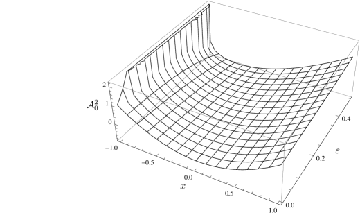
Figure 1: The solution $\mathcal{A}^{l_{0}}_{0}$  of (2) for $l_{0}=2\,,\,n=0$, is represented as a function of $x$, $-1\leq x\leq 1$ for $0\leq\varepsilon<\frac{1}{2}$. We set $a^{2}_{0}=1$.

In figure 2 the solution $\;\mathcal{B}^{l_{0}}_{0+1}$ for $l_{0}=2,n=0,$ is presented. It determines, together with $\mathcal{A}^{2}_{0}$ from figure 1, the spinor state (34) with the mass $m\,\rho_{0}=\sqrt{2\,(3-2\varepsilon)}$. The solution $\mathcal{B}^{2}_{0+1}$ changes from $\mathcal{B}^{2}_{0+1}=\frac{i\sqrt{6}}{5}\,\frac{1}{\sqrt{1-x^{2}}}\times[P^{3}_{0}-P^{1}_{0}]\,$ for $\varepsilon=0$ to the function $\mathcal{B}^{2_{0}}_{0+1}=\frac{i(1+x)^{-\varepsilon}}{\sqrt{2(3-2\varepsilon)}\,\sqrt{1-x^{2}}}\times\,[\frac{6}{5}\,(P^{3}_{0}-P^{1}_{0})+\frac{2\varepsilon}{2-\varepsilon}\,(P^{2}_{0}-P^{0}_{0})]$ for $0\leq\varepsilon<\frac{1}{2}$. While $\;\mathcal{A}^{2}_{0}$ is infinite at $x=-1$, but integrable, $\;\mathcal{B}^{l_{0}}_{0+1}$ is finite in the whole interval for any $l_{0}\,,n=0$, due to the fact that $((P^{l+1}_{0}-P^{l-1}_{0}))|_{x=-1}=0$. This is no longer true if $n\neq 0$.

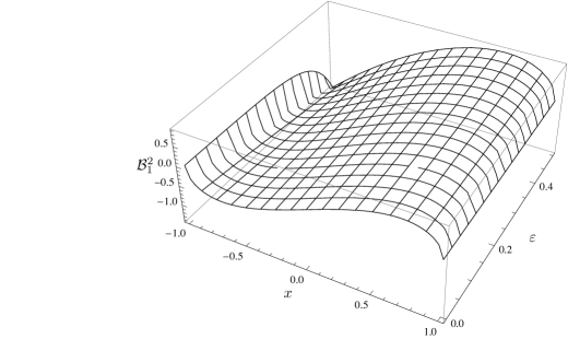
Figure 2: The solution $\mathcal{B}^{2}_{0+1}$ of (2), which together with $\mathcal{A}^{2}_{0}$ from figure 1 determines a spinor state (34) with the mass $(m\,\rho_{0})^{2}=2(3-2\varepsilon)$, is presented as a function of $x$, $-1\leq x\leq 1$ for $0\leq\varepsilon<\frac{1}{2}$.

In figures 3 and 4 the functions $\mathcal{A}^{4}_{0}$ and $\mathcal{B}^{4}_{0+1}$, which solve for $l_{0}=4,n=0$, equation  (2), are presented. The zeros of both functions for three particular values of $\varepsilon$ can be read in figures 5, 6.

Although the functions $\mathcal{A}^{l_{0}}_{n}$ and $\mathcal{B}^{l_{0}}_{n+1}$ are infinite at $x=-1$ for all $\varepsilon\neq 0$, $\mathcal{A}^{l_{0}}_{n}$ for any $n\leq l_{0}$ and $\mathcal{B}^{l_{0}}_{n+1}$ for any $n\neq 0$ and $n\leq l_{0}$, the solutions are all square integrable for $0\leq\varepsilon<\frac{1}{2}$ in the interval $-1\leq x\leq 1$ and correspondingly normalisable.

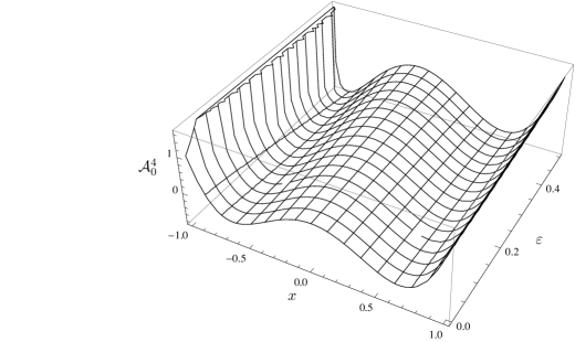
Figure 3: $\mathcal{A}^{4}_{0}$, the solution of (2) for $l_{0}=4\,,n=0$, is presented as a function of $x$, $-1\leq x\leq 1$ for $0\leq\varepsilon<\frac{1}{2}$. We set $a^{4}_{0}=1$.

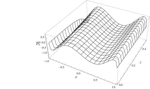
Figure 4: $\mathcal{B}^{4}_{0+1}$, which together with $\mathcal{A}^{4}_{0}$ from figure 3 determines a spinor state (34) with the mass $(m\rho_{0})^{2}=4(5-2\varepsilon)$, is presented as a function of $x$, $-1\leq x\leq 1$ for $0\leq\varepsilon<\frac{1}{2}$.

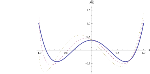
Figure 5: $\mathcal{A}^{4}_{0}$, the solution of (2) for $l_{0}=4$ from figure 3 for three values of $\varepsilon=0,\,0.25,\,0.49$ (thick, dashed and dotted, respectively) is presented as a function of $x$, $-1\leq x\leq 1$.

Figure 6: $\mathcal{B}^{4}_{0}$ from figure 4 is presented as a function of $x$, $-1\leq x\leq 1$, for three values of $\varepsilon=0,\,0.25,\,0.49$ (thick, dashed and dotted, respectively).

In figures 7 and  8 we plot $\mathcal{A}^{2}_{1}$ and $\mathcal{B}^{2}_{1+1}\,$, the solutions (12) of (2, 2) for $l_{0}=2$ and $n=1$, as functions of $x$, $-1\leq x\leq 1$ and $\varepsilon$, $0\leq\varepsilon<\frac{1}{2}$. The mass is independent of the choice of $n$ and therefore equal to $m\,\rho_{0}=\sqrt{2(3-2\varepsilon)}$. One finds $\mathcal{A}^{2}_{1}=(1+x)^{-\varepsilon}\,a^{2}_{1}\,(P^{2}_{1}+\frac{9\varepsilon}{2-\varepsilon}\,P^{1}_{1})$ and $\mathcal{B}^{2}_{1+1}=\frac{i(1+x)^{-\varepsilon}}{\sqrt{2(3-2\varepsilon)}\,\sqrt{1-x^{2}}}\times\,[\frac{4}{5}\,P^{3}_{1}-(1-\frac{3\varepsilon}{2-\varepsilon})\,P^{2}_{1}-9\,(\frac{1}{5}+\frac{\varepsilon}{2-\varepsilon})\,P^{1}_{1}]$.

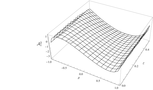
Figure 7: $\mathcal{A}^{2}_{1}$, the solution of (2) for $l_{0}=2$ and $n=1$, is presented as a function of $x$, $\,-1\leq x\leq 1$, for $\,0\leq\varepsilon<\frac{1}{2}$. We set $a^{2}_{0}=1$.

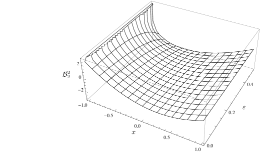
Figure 8: $\mathcal{B}^{2}_{1+1}$, which together with $\mathcal{A}^{2}_{1}$ from figure 7 determines a spinor state (34) with the mass $(m\,\rho_{0})^{2}=2(3-2\varepsilon)$, is represented as a function of $x$, $-1\leq x\leq 1$ for $0\leq\varepsilon<\frac{1}{2}$.

Let us conclude the paper by repeating briefly what we have succeeded to do. We prove that the normalisable solutions of equations of motion (7) can be found for an interval $0\leq\varepsilon<\frac{1}{2}$ of the parameter $\varepsilon=\frac{1}{2}-F$, if a spinor lives on a manifold $M^{1+5}$, which breaks into $M^{1+3}\times$ an infinite disc, with the zweibein of (1) curving the disc into an almost $S^{2}$ and with the spin connection field (5) which allows on such a disc a massless spinor of only one handedness. The solutions were found by using the ansatz (32), with the expansion over the associate Legendre polynomials, which offer normalisable solutions only for a finite sum, that is up to $l_{0}$, $\,l\leq l_{0}$. For each $l_{0}=0,1,2,\dots$ and each chosen value of $0\leq\varepsilon<\frac{1}{2}$ a discrete mass spectrum ($(m\,\rho_{0})^{2}=l_{0}\,(l_{0}+1-2\varepsilon)$) follows, determined by $\rho_{0}$. There is the gap between the massless and massive states as long as the zweibein and the spin connection remain unchanged. Correspondingly, because of the gap, the massless state can not go continuously into the massive ones for any $0\leq<\frac{1}{2}$. High enough temperatures in comparison with $\frac{1}{\rho_{0}}$ can, however, since the space is non compact, cause the change of the fields on the infinite disc and correspondingly also of the spectrum. But as long as the temperature is low, we take it zero in this paper, the massless spinor is (on the tree level) mass protected and also chirally coupled to the corresponding Kaluza-Klein gauge field.

The proof presented in this paper is a step to the proof that one can escape from the ”no-go theorem” of Witten [13], that is that one can guarantee the masslessness of spinors and their chiral coupling to the Kaluza-Klein[like] gauge fields when breaking the symmetry from the $d$-dimensional one to $M^{(1+3)}\times M^{d-4}$ space.

The presented way of searching for solutions of the coupled equations (2) of the first order, leading to the differential equations of the second order (2, 2), is by itself a nice presentation of how can one find normalisable solutions of quite complicated differential equations of the second order.

Appendix A The technique for representing spinors [14, 15], taken from [19]

The technique [14, 15] can be used to construct a spinor basis for any dimension $d$ and any signature in an easy and transparent way. Equipped with the graphic presentation of basic states, the technique offers an elegant way to see all the quantum numbers of states with respect to the Lorentz groups, as well as transformation properties of the states under any Clifford algebra object.

The objects $\gamma^{a}$ have properties

$$\{\gamma^{a},\gamma^{b}\}_{+}=2\eta^{ab}\,I,$$ (41)

for any $d$, even or odd. $I$ is the unit element in the Clifford algebra.

The Clifford algebra objects $S^{ab}$ close the algebra of the Lorentz group

$$S^{ab}: = (i/4)(\gamma^{a}\gamma^{b}-\gamma^{b}\gamma^{a})\,,$$

$$\{S^{ab},S^{cd}\}_{-} = i(\eta^{ad}S^{bc}+\eta^{bc}S^{ad}-\eta^{ac}S^{bd}-\eta^{bd}S^{ac})\,.$$ (42)

The “Hermiticity” property for $\gamma^{a}$’s

$$\gamma^{a\dagger}=\eta^{aa}\gamma^{a}\,,$$ (43)

is assumed in order that $\gamma^{a}$ are compatible with (41) and formally unitary, i.e. $\gamma^{a\,\dagger}\,\gamma^{a}=I$.

One finds from (43) that $(S^{ab})^{\dagger}=\eta^{aa}\eta^{bb}S^{ab}$.

The Cartan subalgebra of the algebra is chosen as follows

$$S^{03},S^{12},S^{56},\cdots,S^{d-1\;d},\quad{\rm if}\quad d = 2n\geq 4,$$

$$S^{03},S^{12},\cdots,S^{d-2\;d-1},\quad{\rm if}\quad d = (2n+1)>4\,.$$ (44)

The choice for the Cartan subalgebra in $d<4$ is straightforward. It is useful to define one of the Casimirs of the Lorentz group - the handedness $\Gamma$ ($\{\Gamma,S^{ab}\}_{-}=0$) in any $d$

$$\Gamma^{(d)}: = (i)^{d/2}\;\;\;\;\;\;\prod_{a}\quad(\sqrt{\eta^{aa}}\gamma^{a}),\quad{\rm if}\quad d=2n,$$

$$\Gamma^{(d)}: = (i)^{(d-1)/2}\;\prod_{a}\quad(\sqrt{\eta^{aa}}\gamma^{a}),\quad{\rm if}\quad d=2n+1\,.$$ (45)

The product of $\gamma^{a}$’s in the ascending order with respect to the index $a$: $\gamma^{0}\gamma^{1}\cdots\gamma^{d}$ is understood. It follows from (43) for any choice of the signature $\eta^{aa}$ that $\Gamma^{\dagger}=\Gamma,\;\Gamma^{2}=I.$ For $d$ even the handedness anticommutes with the Clifford algebra objects $\gamma^{a}$ ($\{\gamma^{a},\Gamma\}_{+}=0$), while for $d$ odd it commutes with $\gamma^{a}$ ($\{\gamma^{a},\Gamma\}_{-}=0$).

To make the technique simple the graphic presentation is introduced

$$\stackrel{{\scriptstyle ab}}{{(k)}}: = \frac{1}{2}(\gamma^{a}+\frac{\eta^{aa}}{ik}\gamma^{b})\,,\quad\quad\stackrel{{\scriptstyle ab}}{{[k]}}:=\frac{1}{2}(1+\frac{i}{k}\gamma^{a}\gamma^{b})\,,$$

$$\stackrel{{\scriptstyle+}}{{\circ}}: = \frac{1}{2}(1+\Gamma)\,,\quad\quad\stackrel{{\scriptstyle-}}{{\bullet}}:=\frac{1}{2}(1-\Gamma),$$ (46)

where $k^{2}=\eta^{aa}\eta^{bb}$. One can easily check by taking into account the Clifford algebra relation (41) and the definition of $S^{ab}$ (A) that if one multiplies from the left hand side by $S^{ab}$ the Clifford algebra objects $\stackrel{{\scriptstyle ab}}{{(k)}}$ and $\stackrel{{\scriptstyle ab}}{{[k]}}$, it follows that

$$S^{ab}\,\stackrel{{\scriptstyle ab}}{{(k)}}=\frac{1}{2}\,k\,\stackrel{{\scriptstyle ab}}{{(k)}}\,,\quad\quad S^{ab}\,\stackrel{{\scriptstyle ab}}{{[k]}}=\frac{1}{2}\,k\,\stackrel{{\scriptstyle ab}}{{[k]}}\,,$$ (47)

which means that we get the same objects back multiplied by the constant $\frac{1}{2}k$. This also means that when $\stackrel{{\scriptstyle ab}}{{(k)}}$ and $\stackrel{{\scriptstyle ab}}{{[k]}}$ act from the left hand side on a vacuum state $|\psi_{0}\rangle$ the obtained states are the eigenvectors of $S^{ab}$. One can further recognize that $\gamma^{a}$ transform $\stackrel{{\scriptstyle ab}}{{(k)}}$ into $\stackrel{{\scriptstyle ab}}{{[-k]}}$, never to $\stackrel{{\scriptstyle ab}}{{[k]}}$:

$$\gamma^{a}\stackrel{{\scriptstyle ab}}{{(k)}} = \eta^{aa}\stackrel{{\scriptstyle ab}}{{[-k]}},\;\gamma^{b}\stackrel{{\scriptstyle ab}}{{(k)}}=-ik\stackrel{{\scriptstyle ab}}{{[-k]}},\;\gamma^{a}\stackrel{{\scriptstyle ab}}{{[k]}}=\stackrel{{\scriptstyle ab}}{{(-k)}},\;\gamma^{b}\stackrel{{\scriptstyle ab}}{{[k]}}=-ik\eta^{aa}\stackrel{{\scriptstyle ab}}{{(-k)}}\,.$$ (48)

From (48) it follows

$$S^{ac}\stackrel{{\scriptstyle ab}}{{(k)}}\stackrel{{\scriptstyle cd}}{{(k)}} = -\frac{i}{2}\eta^{aa}\eta^{cc}\stackrel{{\scriptstyle ab}}{{[-k]}}\stackrel{{\scriptstyle cd}}{{[-k]}}\,,$$

$$S^{ac}\stackrel{{\scriptstyle ab}}{{[k]}}\stackrel{{\scriptstyle cd}}{{[k]}} = \frac{i}{2}\stackrel{{\scriptstyle ab}}{{(-k)}}\stackrel{{\scriptstyle cd}}{{(-k)}}\,,$$

$$S^{ac}\stackrel{{\scriptstyle ab}}{{(k)}}\stackrel{{\scriptstyle cd}}{{[k]}} = -\frac{i}{2}\eta^{aa}\stackrel{{\scriptstyle ab}}{{[-k]}}\stackrel{{\scriptstyle cd}}{{(-k)}}\,,$$

$$S^{ac}\stackrel{{\scriptstyle ab}}{{[k]}}\stackrel{{\scriptstyle cd}}{{(k)}} = \frac{i}{2}\eta^{cc}\stackrel{{\scriptstyle ab}}{{(-k)}}\stackrel{{\scriptstyle cd}}{{[-k]}}\,.$$ (49)

Let us deduce some useful relations

$$\stackrel{{\scriptstyle ab}}{{(k)}}\stackrel{{\scriptstyle ab}}{{(k)}} = 0\,,\quad\quad\stackrel{{\scriptstyle ab}}{{(k)}}\stackrel{{\scriptstyle ab}}{{(-k)}}=\eta^{aa}\stackrel{{\scriptstyle ab}}{{[k]}}\,,\quad\stackrel{{\scriptstyle ab}}{{(-k)}}\stackrel{{\scriptstyle ab}}{{(k)}}=\eta^{aa}\stackrel{{\scriptstyle ab}}{{[-k]}}\,,\quad\stackrel{{\scriptstyle ab}}{{(-k)}}\stackrel{{\scriptstyle ab}}{{(-k)}}=0\,,$$

$$\stackrel{{\scriptstyle ab}}{{[k]}}\stackrel{{\scriptstyle ab}}{{[k]}} = \stackrel{{\scriptstyle ab}}{{[k]}}\,,\quad\quad\stackrel{{\scriptstyle ab}}{{[k]}}\stackrel{{\scriptstyle ab}}{{[-k]}}=0\,,\;\;\quad\quad\quad\stackrel{{\scriptstyle ab}}{{[-k]}}\stackrel{{\scriptstyle ab}}{{[k]}}=0\,,\;\;\quad\quad\quad\quad\stackrel{{\scriptstyle ab}}{{[-k]}}\stackrel{{\scriptstyle ab}}{{[-k]}}=\stackrel{{\scriptstyle ab}}{{[-k]}}\,,$$

$$\stackrel{{\scriptstyle ab}}{{(k)}}\stackrel{{\scriptstyle ab}}{{[k]}} = 0\,,\quad\quad\quad\stackrel{{\scriptstyle ab}}{{[k]}}\stackrel{{\scriptstyle ab}}{{(k)}}=\stackrel{{\scriptstyle ab}}{{(k)}}\,,\quad\quad\quad\stackrel{{\scriptstyle ab}}{{(-k)}}\stackrel{{\scriptstyle ab}}{{[k]}}=\stackrel{{\scriptstyle ab}}{{(-k)}}\,,\quad\quad\quad\stackrel{{\scriptstyle ab}}{{(-k)}}\stackrel{{\scriptstyle ab}}{{[-k]}}=0\,,$$

$$\stackrel{{\scriptstyle ab}}{{(k)}}\stackrel{{\scriptstyle ab}}{{[-k]}} = \stackrel{{\scriptstyle ab}}{{(k)}}\,,\quad\quad\stackrel{{\scriptstyle ab}}{{[k]}}\stackrel{{\scriptstyle ab}}{{(-k)}}=0,\quad\quad\quad\stackrel{{\scriptstyle ab}}{{[-k]}}\stackrel{{\scriptstyle ab}}{{(k)}}=0\,,\quad\quad\quad\quad\stackrel{{\scriptstyle ab}}{{[-k]}}\stackrel{{\scriptstyle ab}}{{(-k)}}=\stackrel{{\scriptstyle ab}}{{(-k)}}.$$ (50)

We recognize in the first equation of the first row and the first equation of the second row the demonstration of the nilpotent and the projector character of the Clifford algebra objects $\stackrel{{\scriptstyle ab}}{{(k)}}$ and $\stackrel{{\scriptstyle ab}}{{[k]}}$, respectively. Recognizing that

$$\stackrel{{\scriptstyle ab}}{{(k)}}^{\dagger}=\eta^{aa}\stackrel{{\scriptstyle ab}}{{(-k)}}\,,\quad\stackrel{{\scriptstyle ab}}{{[k]}}^{\dagger}=\stackrel{{\scriptstyle ab}}{{[k]}}\,,$$ (51)

a vacuum state $|\psi_{0}>$ can be defined so that it follows

$$<\;\stackrel{{\scriptstyle ab}}{{(k)}}^{\dagger}\stackrel{{\scriptstyle ab}}{{(k)}}\;>=1\,,\quad\quad<\;\stackrel{{\scriptstyle ab}}{{[k]}}^{\dagger}\stackrel{{\scriptstyle ab}}{{[k]}}\;>=1\,.$$ (52)

Taking into account the above equations it is easy to find a Weyl spinor irreducible representation for $d$-dimensional space, with $d$ even or odd.

For $d$ even we simply make a starting state as a product of $d/2$, let us say, only nilpotents $\stackrel{{\scriptstyle ab}}{{(k)}}$, one for each $S^{ab}$ of the Cartan subalgebra elements (44), applying it on an (unimportant) vacuum state. For $d$ odd the basic states are products of $(d-1)/2$ nilpotents and a factor $(1\pm\Gamma)$. Then the generators $S^{ab}$, which do not belong to the Cartan subalgebra, being applied on the starting state from the left, generate all the members of one Weyl spinor.

$$\stackrel{{\scriptstyle 0d}}{{(k_{0d})}}\stackrel{{\scriptstyle 12}}{{(k_{12})}}\stackrel{{\scriptstyle 35}}{{(k_{35})}}\cdots\stackrel{{\scriptstyle d-1\;d-2}}{{(k_{d-1\;d-2})}}\psi_{0}$$

$$\stackrel{{\scriptstyle 0d}}{{[-k_{0d}]}}\stackrel{{\scriptstyle 12}}{{[-k_{12}]}}\stackrel{{\scriptstyle 35}}{{(k_{35})}}\cdots\stackrel{{\scriptstyle d-1\;d-2}}{{(k_{d-1\;d-2})}}\psi_{0}$$

$$\stackrel{{\scriptstyle 0d}}{{[-k_{0d}]}}\stackrel{{\scriptstyle 12}}{{(k_{12})}}\stackrel{{\scriptstyle 35}}{{[-k_{35}]}}\cdots\stackrel{{\scriptstyle d-1\;d-2}}{{(k_{d-1\;d-2})}}\psi_{0}$$

$$\vdots$$

$$\stackrel{{\scriptstyle 0d}}{{[-k_{0d}]}}\stackrel{{\scriptstyle 12}}{{(k_{12})}}\stackrel{{\scriptstyle 35}}{{(k_{35})}}\cdots\stackrel{{\scriptstyle d-1\;d-2}}{{[-k_{d-1\;d-2}]}}\psi_{0}$$

$$\stackrel{{\scriptstyle od}}{{(k_{0d})}}\stackrel{{\scriptstyle 12}}{{[-k_{12}]}}\stackrel{{\scriptstyle 35}}{{[-k_{35}]}}\cdots\stackrel{{\scriptstyle d-1\;d-2}}{{(k_{d-1\;d-2})}}\psi_{0}$$

$$\vdots$$ (53)

All the states have the handedness $\Gamma$, since $\{\Gamma,S^{ab}\}-{+}=0$. States, belonging to one multiplet with respect to the group $SO(q,d-q)$, that is to one irreducible representation of spinors (one Weyl spinor), can have any phase. We made a choice of the simplest one, taking all phases equal to one.

The above graphic representation demonstrates that for $d$ even all the states of one irreducible Weyl representation of a definite handedness follow from a starting state, which is, for example, a product of nilpotents $\stackrel{{\scriptstyle ab}}{{(k_{ab})}}$, by transforming all possible pairs of $\stackrel{{\scriptstyle ab}}{{(k_{ab})}}\stackrel{{\scriptstyle mn}}{{(k_{mn})}}$ into $\stackrel{{\scriptstyle ab}}{{[-k_{ab}]}}\stackrel{{\scriptstyle mn}}{{[-k_{mn}]}}$. There are $S^{am},S^{an},S^{bm},S^{bn}$, which do this. The procedure gives $2^{(d/2-1)}$ states. A Clifford algebra object $\gamma^{a}$ being applied from the left hand side, transforms a Weyl spinor of one handedness into a Weyl spinor of the opposite handedness. Both Weyl spinors form a Dirac spinor.

For $d$ odd a Weyl spinor has besides a product of $(d-1)/2$ nilpotents or projectors also either the factor $\stackrel{{\scriptstyle+}}{{\circ}}:=\frac{1}{2}(1+\Gamma)$ or the factor $\stackrel{{\scriptstyle-}}{{\bullet}}:=\frac{1}{2}(1-\Gamma)$. As in the case of $d$ even, all the states of one irreducible Weyl representation of a definite handedness follow from a starting state, which is, for example, a product of $(1+\Gamma)$ and $(d-1)/2$ nilpotents $\stackrel{{\scriptstyle ab}}{{(k_{ab})}}$, by transforming all possible pairs of $\stackrel{{\scriptstyle ab}}{{(k_{ab})}}\stackrel{{\scriptstyle mn}}{{(k_{mn})}}$ into $\stackrel{{\scriptstyle ab}}{{[-k_{ab}]}}\stackrel{{\scriptstyle mn}}{{[-k_{mn}]}}$. But $\gamma^{a}$’s, being applied from the left hand side, do not change the handedness of the Weyl spinor, since $\{\Gamma,\gamma^{a}\}_{-}=0$ for $d$ odd. A Dirac and a Weyl spinor are for $d$ odd identical and a ”family” has accordingly $2^{(d-1)/2}$ members of basic states of a definite handedness.

We shall speak about left handedness when $\Gamma=-1$ and about right handedness when $\Gamma=1$ for either $d$ even or odd.

Making a choice of the Cartan subalgebra set of the algebra $S^{ab}$

$$S^{03},S^{12},S^{56}\,,$$ (54)

a left handed ($\Gamma^{(1,5)}=-1$) eigen state of all the members of the Cartan subalgebra can be written as

$$\stackrel{{\scriptstyle 03}}{{(+i)}}\stackrel{{\scriptstyle 12}}{{(+)}}\stackrel{{\scriptstyle 56}}{{(+)}}|\psi\rangle=\frac{1}{2^{3}}(\gamma^{0}-\gamma^{3})(\gamma^{1}+i\gamma^{2})|(\gamma^{5}+i\gamma^{6})|\psi\rangle\,.$$ (55)

This state is an eigen state of all $S^{ab}$ which are members of the Cartan subalgebra (54).

Below some useful relations [14] are presented

$$N^{\pm}_{+} = N^{1}_{+}\pm i\,N^{2}_{+}=-\stackrel{{\scriptstyle 03}}{{(\mp i)}}\stackrel{{\scriptstyle 12}}{{(\pm)}}\,,\quad N^{\pm}_{-}=N^{1}_{-}\pm i\,N^{2}_{-}=\stackrel{{\scriptstyle 03}}{{(\pm i)}}\stackrel{{\scriptstyle 12}}{{(\pm)}}\,,$$

Appendix B Useful relations among Legendre polynomials

We present in this appendix some useful relations, some of them are well known [17]

$$\quad xP^{l}_{n} = \frac{1}{2l+1}\left[(l+n)P^{l-1}_{n}+(l-n+1)P^{l+1}_{n}\right]\,,$$ (57)

$$(2l+1)\sqrt{1-x^{2}}P^{l}_{n-2}=P^{l-1}_{n-1}-P^{l+1}_{n-1}\,,$$

$$(2l+1)\sqrt{1-x^{2}}P^{l}_{n}=(l-n+2)(l-n+1)P^{l+1}_{n-1}$$

$$-(l+n)(l+n-1)P^{l-1}_{n-1}\,,$$ (58)

$$(1-x^{2})\frac{d}{dx}P^{l}_{n} = \frac{1}{2l+1}\left[(l+n)(l+1)P^{l-1}_{n}-l(l-n+1)P^{l+1}_{n}\right]\,.$$ (59)

Others follow with some effort from the above ones.

$$(1-x^{2})P^{l}_{n}=\frac{1}{2l+1}\biggl{\{}\left[2l+1-\frac{(l+n)(l-n)}{2l-1}-\frac{(l-n+1)(l+n+1)}{2l+3}\right]P^{l}_{n}$$

$${}-\frac{(l+n)(l+n-1)}{2l-1}P^{l-2}_{n}-\frac{(l-n+1)(l-n+2)}{2l+3}P^{l+2}_{n}\biggr{\}}\,,$$ (60)

$$\frac{1}{\sqrt{1-x^{2}}}P^{l}_{n}=-\frac{1}{2n}\left((l-n+2)(l-n+1)P^{l+1}_{n-1}+P^{l+1}_{n+1}\right)\,,$$ (61)

$$\frac{1}{\sqrt{1-x^{2}}}P^{l}_{n}=-\frac{1}{2n}\left((l+n)(l+n-1)P^{l-1}_{n-1}+P^{l-1}_{n+1}\right)\,.$$ (62)

Any function $f$, continuous on the open interval $(-1,1)$ and square integrable in the closed interval ($\int^{1}_{-1}\,dx\,|f|^{2}$), can be expanded in terms of associate Legendre functions $P^{l}_{n}$:

$$f(x) = \sum_{l\geq n}\,c_{l}^{n}\,P^{l}_{n}\,(x)\,,$$

$$c_{l}^{n} = \frac{2l+1}{2}\,\frac{(l-n)!}{(l+n)!}\,\int_{-1}^{1}\,f(x)\,P^{l}_{n}\,(x)\,dx\,.$$ (63)

Appendix C Recursive relations for the ansatzes $\mathcal{A}_{n}=\sum_{l\geq n}\,\alpha^{l}_{n}P^{l}_{n}$ and $\mathcal{B}_{n+1}=\sum_{l\geq n+1}\beta^{l}_{n+1}P^{l}_{n+1}$

Using relations from B it is not too difficult to find the recurrence relations for $\alpha^{l}_{n}$ when the ansatz $\mathcal{A}_{n}=\sum_{l\geq n}\,\alpha^{l}_{n}P^{l}_{n}$ is used in equation

$$(1-x^{2})\frac{d^{2}}{dx^{2}}\mathcal{A}_{n}-2x\frac{d}{dx}\mathcal{A}_{n}+(m\rho_{0})^{2}\mathcal{A}_{n}$$

$$-\left\{\frac{n^{2}}{1-x^{2}}+\frac{1}{1+x}\varepsilon(1+x+2n)+\varepsilon^{2}\frac{1-x}{1+x}\right\}\mathcal{A}_{n}=0\,.$$ (64)

One finds

$$\alpha^{l+1}_{n}\frac{l+n+1}{2l+3}\left[(m\rho_{0})^{2}-(l+1)(l+2)-\varepsilon(1-\varepsilon)\right]=$$

$$-\alpha^{l}_{n}\left[(m\rho_{0})^{2}-l(l+1)-\varepsilon(1+\varepsilon+2n)\right]$$

$$-\alpha^{l-1}_{n}\frac{l-n}{2l-1}\left[(m\rho_{0})^{2}-(l-1)l-\varepsilon(1-\varepsilon)\right]\,.$$ (65)

Similarly one finds recurrence relations for $\beta^{l}_{n+1}$ when using the ansatz $\mathcal{B}_{n+1}=\sum_{l\geq n+1}\beta^{l}_{n+1}P^{l}_{n+1}$ in equation

$$(1-x^{2})\frac{d^{2}}{dx^{2}}\mathcal{B}_{n+1}-2x\frac{d}{dx}\mathcal{B}_{n+1}+(m\rho_{0})^{2}\mathcal{B}_{n+1}$$

$$+\left\{-\frac{(n+1)^{2}}{1-x^{2}}+\frac{2n(1-\varepsilon)}{1+x}+\varepsilon(1-\varepsilon)\frac{1-x}{1+x}\right\}\mathcal{B}_{n+1}=0\,.$$ (66)

One obtains

$$\beta^{l+1}_{n+1}\frac{l+n+2}{2l+3}\left[(m\rho_{0})^{2}-(l+1)(l+2)-\varepsilon(1-\varepsilon)\right]=$$

$$-\beta^{l}_{n+1}\left[(m\rho_{0})^{2}-l(l+1)+(1-\varepsilon)(\varepsilon+2n)\right]$$

$$-\beta^{l-1}_{n+1}\frac{l-n-1}{2l-1}\left[(m\rho_{0})^{2}-(l-1)l-\varepsilon(1-\varepsilon)\right]\,.$$ (67)

The two ansatzes are not really useful, since it is very difficult to evaluate for which values of $(m\rho_{0})^{2}$ are the solutions square integrable. The ansatzes from (32, 2) are much more appropriate offering us the solutions in quite an elegant way.

References

[1] Lukman D, Mankoč Borštnik N S and Nielsen H B
2011 New J. Phys.13 (2011) 103027
[2] Kaluza T 1921 Sitzungsber.Preuss.Akad.Wiss.Berlin, Math.Phys.K1 966,
Klein ) 1926 Z.Phys.37 895
[3] Georgi H and Glashow S L 1974 Phys. Rev. Lett.32 438
[4] Cho Y M 1975 J. Math. Phys.16 2029,
Cho Y M and Freund P G O 1975 Phys. Rev.D 12 1711
[5] Zee A 1981 Proc. 1st Kyoto Summer Institute on
Grand Unified Theories and Related Topics (Kyoto) ed M Konuma and T Kaskawa
(Singapore: World Scientific)
[6] Salam A and Strathdee J 1982 Ann. Phys., NY141 316
[7] Mecklenburg W 1984 Fortschr. Phys.32 207
[8] Duff M, Nilsson, B and Pope C 1984 Phys. Rep. C C 130 1,
Duff M, Nilsson B, Pope C and Warner N 1984 Phys. Lett.B 149 60
[9] Randjbar-Daemi S, Salam A and Strathdee J 1984 Nucl. Phys.B 242 447
[10] Wetterich C 1985 The 2nd Jerusalem Winter School on Theoretical Physics
CERN-TH4190/85 and references therein, Wetterich C 1985 Nucl. Phys.B 253 261,
Wetterich C 1984 Nucl. Phys.B 234 413
[11] The authors of the works presented in 1983 An Introduction to Kaluza-Klein
Theories ed H C Lee (Singapore: World Scientific)
[12] Horvath Z, Palla L, Crammer E and Scherk J 1977 Nucl. Phys.B
127 57
[13] Witten E 1981 Nucl. Phys.B 186 412; Witten E 1883 Princeton Technical Rep. PRINT -83-1056, October 1983
[14] Mankoč Borštnik N S 1992 Phys. Lett.B 292 25,
Mankoč Borštnik N S 1993 J. Math. Phys.34 3731,
Mankoč Borštnik N S2001 Int. J. Theor. Phys.40 315,
Mankoč Borštnik N S 1995 Modern Phys. Lett. A 10 587,
Borštnik A and Mankoč Borštnik N S 2004 (Preprint
hep-ph/0401043), Borštnik A and Mankoč Borštnik N S 2004
(Preprint hep-ph/0401055) pp 27–51,
Borštnik A and Mankoč Borštnik N S 2002 (Preprint hep-ph/0301029)
Borštnik A and Mankoč Borštnik N S 2006Phys. Rev.D 74
073013 (Preprint hep-ph/0512062),
Bregar G, Breskvar M, Lukman D and Mankoč Borštnik N S 2007
(Preprint hep-ph/0711.4681) pp 53–70,
Bregar G, Breskvar M, Lukman D and Mankoč Borštnik N S 2008
New J. Phys.10 093002,
Breskvar M, Lukman D and Mankoč Borštnik N S 2006 (Preprint hep-ph/0606159,
Bregar G, Breskvar M, Lukman D and Mankoč Borštnik N S 2007
(Preprint hep-ph/07082846),
Breskvar M, Lukman D and Mankoč Borštnik N S 2006 (Preprint hep-ph/0612250) pp25–50
[15] Mankoč Borštnik N S and Nielsen H B 2002
J. Math. Phys.43 5782, Mankoč Borštnik N S and Nielsen H B 2001,
Mankoč Borštnik N S and Nielsen H B 2001 (Preprint hep-th/0111257),
Mankoč Borštnik N S and Nielsen H B 2003 J. Math. Phys.44 4817,
Mankoč Borštnik N S and Nielsen H B 2003 (Preprint hep-th/0303224)
[16] Mankoč Borštnik N S and Nielsen H B 2006
Phys. Lett.B 633 771–5, Mankoč Borštnik N S and Nielsen H B
2003 (Preprint hep-th/0311037), Mankoč Borštnik N S and
Nielsen H B 2005 (Preprint hep-th/0509101),
Mankoč Borštnik N S and Nielsen H B 2007 Phys. Lett.B 644 198–202,
Mankoč Borštnik N S and Nielsen H B 2006 (Preprint hep-th/0608006),
Mankoč Borštnik N S and Nielsen H B 2008 Phys. Lett.B 663 265–96,
Mankoč Borštnik N S, Nielsen H B and Lukman D 2004
(Preprint hep-ph/0412208)
[17] Wang Z X and Guo D R 1989 Special Functions (Singapore: Worls Scientific)
pp255–8
[18] Tikhonov A N and Samarskii A A 1963 Equations of Mathematical Physics,
(International Series of Monographs on Pure and Applied
Mathematics vol 39) (Oxford etc.: Pergamon Press)
[19] Mankoč Borštnik N S 2010 (Preprint arxiv:1011.5765),
Mankoč Borštnik N S 2010 (Preprint arXiv:1012.0224) pp105–30