Finite size scaling on the phase diagram of QCD

Abstract

In the last years there has been remarkable progress in the comparison of experimental data on the shape of event-by-event distributions of conserved quantities and lattice thermodynamic predictions based on the grand canonical ensemble. In this talk we discuss how the QCD crossover temperature and the freezeout curve are extracted from the analysis of fluctuations. We report that one can also go further and locate the QCD critical point at $\mu\simeq 2T_{c}$. We also list the systematics which must be brought under control in future.

I Introduction

In the last years a major development occurred in the experimental study of the phase diagram of QCD. It was established that certain measures of the shape of the distribution of event-to-event fluctuations of conserved quantities cpod09 which were predicted through lattice QCD simulations shape agreed well with experimental observations in relativistic heavy-ion collisions star .

The Maclaurin series expansion of the pressure,

$$\frac{1}{T^{4}}P(t,z)=\frac{P(t,0)}{T^{4}}+\frac{\chi^{(1)}(t,0)}{T^{3}}\,z+\frac{\chi^{(2)}(t,0)}{T^{2}}\,\frac{z^{2}}{2!}+\frac{\chi^{(3)}(t,0)}{T}\,\frac{z^{3}}{3!}+\cdots$$ (1)

(where $t=T/T_{c}$ and $z=\mu/T$, $T$ is the temperature, $\mu$ the quark chemical potential and $T_{c}$ any measure of the location of the QCD cross over at $z=0$) is now the method of choice to construct various extrapolations to finite chemical potential on the lattice ilgti . Eq. (1) is written in a form which emphasizes that dimensionless functions of dimensionless numbers are the output of lattice computations. The $\chi^{(n)}(t,z)$, which are the $n$-th derivatives of $P$ with respect to $\mu$ are called nonlinear susceptibilities (NLS); $\chi^{(1)}$ is the quark number density and $\chi^{(2)}$ the quark number susceptibility gottlieb . The series expansions of the NLS are obtained from eq. (1) by merely taking derivatives with respect to $\mu$. Analysis of the series expansion of $\chi^{(2)}(t,z)/T^{2}$ led to current estimates nt6 of the position of the critical end point of QCD

$$z_{E}=1.8\pm 0.1\qquad{\rm and}\qquad t_{E}=0.94\pm 0.01,$$ (2)

where the choice made in shape ; nt6 was to use for the scale of the temperature, $T_{c}(P)$, at which the Polyakov loop susceptibility peaks. The observables for which agreement between lattice predictions and experiments are demonstrated are the ratios cpod09

$$m_{3}(t,z)=\frac{\chi^{(4)}(t,z)}{\chi^{(3)}(t,z)/T},\qquad\qquad m_{2}(t,z)=\frac{\chi^{(4)}(t,z)}{\chi^{(2)}(t,z)/T^{2}},$$

$$m_{1}(t,z)=\frac{\chi^{(3)}(t,z)/T}{\chi^{(2)}(t,z)/T^{2}},\qquad\qquad m_{0}(t,z)=\frac{\chi^{(2)}(t,z)/T^{2}}{\chi^{(1)}(t,z)/T^{3}},$$ (3)

A development of this kind immediately makes possible other ways of looking at old questions and asking new physics questions: outlining some of these is one purpose of this review. The other is an equally important task: critically examining the assumptions that went into the comparison with a view to making them quantitatively testable. These are the contents of the next two sections.

II Old and new questions

The initial demonstration of the agreement between experimental observation and lattice predictions proceeded in the following way. Lattice simulations predict dimensionless ratios as functions of other dimensionless ratios. In order to make contact with experiment two inputs were needed. The first was the scale of the lattice computations, $T_{c}(P)$. It can be taken from current lattice measurements fodor to be

$$T_{c}(P)=176\pm 3\pm 4{\rm\ MeV},$$ (4)

where the first error comes from finite temperature lattice computations and the second from errors in the setting of scale by matching lattice computations to zero temperature hadron properties. Then lattice computations of $\chi^{(n)}(t,0)$ had to be resummed to give the ratios $m_{i}(t,z)$ along the freezeout curve, $\{T_{f}(\sqrt{S}),\mu_{f}(\sqrt{S})\}$, corresponding to heavy-ion collisions performed with center of mass energy $\sqrt{S}$. This second input, the freezeout curve, was taken from a parametrization of the hadron resonance gas model (HRGM) made through a fit to data on yields of various particles in cleymans .

II.1 Two classic questions

It was pointed out in shape that if reasonable agreement between lattice predictions and data were observed, then by relaxing the above input conditions, these measurements could be used to directly determine either $T_{c}$ or the freezeout curve, or both. These are new ways of putting together lattice predictions and experimental data in order to examine classic questions in the field.

The new program was initiated in glmrx where the freezeout conditions were taken as before and the scale $T_{c}$ was left free to be determined by the lattice predictions and experimental data taken together. Varying the scale $T_{c}(P)$ in order to maximize the agreement between lattice predictions and data gave

$$T_{c}(P)=175^{+1}_{-7}{\rm\ MeV}.$$ (5)

The errors are statistical only. The scale determination using the agreement of lattice predictions with either single hadron properties (eq. 4) or bulk matter (eq. 5, above) agree well, providing the first hard evidence that in lattice gauge theory we have a full theory of non-perturbative QCD.

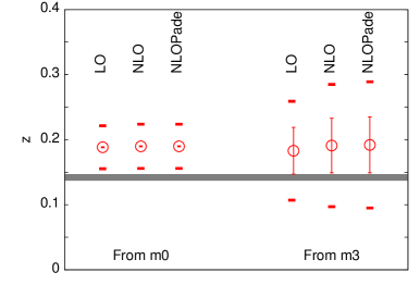
Figure 1: Freeze out parameters at $\sqrt{S}=200$ GeV estimated from the STAR collaboration’s measurements of $m_{0}$ and $m_{3}$. The inner error bars show the effect of statistical errors in data propagated to this parameter (in some cases they are smaller than the size of the symbols), and the outer bars show the effects of systematic errors in data. The gray horizontal band is the statistical error band of the HRGM fit cleymans .

The second piece of physics that one can extract, following the program of shape , is the freezeout point at different $\sqrt{S}$. In an expanding system net yields and fluctuations may freeze out at different points in the phase diagram (as we discuss in the next section), so this is an important measure of the degree of thermalization. The appropriate tools for this follow from eqs. (1) and (3), and some of the steps are given in shape . These lead to the expressions

$$m_{3} = \frac{1}{z}+\frac{4z}{r_{2}^{2}}+O\left(z^{3}\right)=\frac{1}{z}\left[\frac{1+{\cal O}\left(\frac{z}{r_{2}}\right)^{4}}{1-\left(\frac{2z}{r_{2}}\right)^{2}}\right],$$

$$m_{0} = \frac{1}{z}+\frac{2z}{3r_{1}^{2}}+O\left(z^{3}\right)=\frac{1}{z}\left[\frac{1+{\cal O}\left(\frac{z}{r_{1}}\right)^{4}}{1-\frac{2}{3}\left(\frac{z}{r_{1}}\right)^{2}}\right].$$ (6)

Here $r_{1}$ is the leading order estimate of the radius of convergence of the expansion of $\chi^{(2)}/T^{2}$, and $r_{2}$ is the estimate at the next order. The $t$ dependence of the right-hand side is hidden in $r_{1,2}$ whereas the $z$ dependence is explicit. Since the leading dependence on $z$ is the factor of $1/z$, these measurements have been called baryometers karsch . This is, of course, only approximately true (to within 5% at $\sqrt{S}=200$ GeV and to 25% at $\sqrt{S}=62.4$ GeV, as it turns out). In the following we will term the leading order (LO) approximation that is obtained by neglecting all the terms except $1/z$. The next-to-leading order (NLO) approximation comes from keeping the second term in the series. Also shown is the resummation of these into a simple pole (the reason for doing this is given in shape ), an approximation that we term the NLOPadé.

Using the data from star , the LO analysis yields

$$z(\sqrt{S}=200{\rm\ GeV})=\begin{cases}0.1884\pm 0.0007\;(\pm 0.033)&\quad{\rm from\ }m_{0},\\ 0.183\pm 0.036\;(\pm 0.076)&\quad{\rm from\ }m_{3}.\end{cases}$$ (7)

These estimates are shown in Figure 1. The first set of errors is statistical, and obtained neglecting covariance between measurements. The error estimates shown within brackets are similar, but obtained by adding statistical and systematic errors in quadrature. The error analysis should be treated as indicative, since it can be easily improved by experimental collaborations. The freezeout point inferred from HRGM fits is $z=0.142\pm 0.005$, compatible with the above analysis when systematic errors are accounted for. Interestingly, the agreement between freezeout conditions from HRGM and fluctuations improves quite a bit in going from LO to NLO at $\sqrt{S}=62.4$ GeV.

Since there is no pure baryometer, for the NLO analysis one needs to specify $t$, or equivalently the values of $r_{1,2}$. Given the near agreement of the freezeout value of $z$ from yield and fluctuations analyses, it is would seem that no significant error is introduced if we take $t=0.94$ as given in cleymans , instead of determining it through the longer procedure outlined in shape . With this input and the lattice determination of nt6 that $r_{1}=r_{2}=1.8$, one can perform the analysis to orders NLO and NLOPadé. The results are compatible with the estimates in eq. (7) as shown in Figure 1.

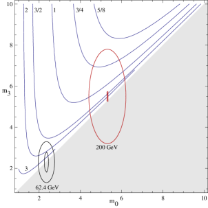
Figure 2: Contours of constant $z_{E}$ in the plane of $m_{0}$ and $m_{3}$. The shaded area below the diagonal is not allowed for any real value of the critical point $z_{E}$. The open curves above the diagonal are contours of $z_{E}$ for the values shown near the lines. The ellipses are $1\sigma$ contours of the measurements at $\sqrt{S}=200$ GeV and $\sqrt{S}=62.4$ GeV star . The outer ellipses are obtained when statistical and systematic errors are added in quadrature, and the inner ellipses show statistical errors only.

Clearly, there are systematic errors in the measurement of yields. However these are not taken into account in the extraction of freezeout conditions. It would be interesting in future to know how large these are, and their influence on the comparison on the two ways of determining the freezeout conditions. Furthermore, when sufficiently large number of cumulants of event-to-event distributions becomes available it may be possible to fit $T_{c}$ and the freezeout conditions simultaneously, thus removing the necessity of external inputs.

II.2 A new question

The beam energy scan at RHIC is examining the exciting new question of the location of the critical point of QCD. The comparisons above show that systems produced at large $\sqrt{S}$ are thermalized. It is expected that if the systems are close to a critical point, then, due to increased relaxation times and correlation lengths, they will not be in local thermal equilibrium berdnikov . So the signal for the critical point will be that of agreement with thermal QCD away from the critical point and lack of agreement near the critical point.

Interestingly enough, it is possible to confirm these results using only data far from a critical point by utilizing an interesting coincidence— that the freezeout value $t(\sqrt{S}=200{\rm\ GeV})=0.94$ is coincidentally very close to $t_{E}$ of eq. (2). At this value of $t$, the series expansion of $m_{0}$ and $m_{3}$ contain $r_{1}=r_{2}=z_{E}$. We have already used this in the above extraction of the freezeout value of $z$ beyond LO.

As a result of this coincidence, we can insert $r_{1}=r_{2}=z_{E}$ in eq. (6), and then extract both $z$ and $z_{E}$ directly from data. This requires a simultaneous fit of data on $m_{0}$ and $m_{3}$ at large $\sqrt{S}$, either top RHIC energy or LHC energies, to the NLOPadé approximation. It is remarkable that under fairly weak assumptions one can extract the location of the critical end point directly from data at the highest collider energies without the direct intervention of lattice predictions.

Using the same data which led to the fits shown in Figure 1 a simultaneous extraction of $z$ and $z_{E}$ gives interesting results. Since the errors on $m_{1}$ are smaller, the best-fit value of $z$ is close to that obtained in the NLOPadé fit of $m_{0}$. Simultaneous use of $m_{0}$ and $m_{3}$ also restricts the errors on $z$ to be smaller than the maximum errors shown in Figure 1.

As for the position of the critical point, in Figure 2 we show contours of constant $z_{E}$ in the plane of $m_{0}$ and $m_{3}$, obtained by solving eq. (6). Whenever $m_{0}=m_{3}$ one can invoke a Poisson description of the data and thereby push the critical point away to infinity. This special case is contained in the contour plots. Since almost all the error ellipses cross the diagonal line in Figure 2, this crude analysis of errors cannot put an upper bound on $z_{E}$. With this treatment we can only give very rough limits on the location of the critical point—

$$z_{E}=2.03_{-1.44}^{+\infty}\qquad{\rm so\ that}\qquad\mu_{E}=355_{-250}^{+\infty}{\rm\ MeV}.$$ (8)

More precisely, one can bound $z_{E}\geq 0.59$ at the 68% confidence level. This is in agreement with the lattice results quoted in eq. (2).

Since it is clear from Figure 2 that the errors are dominated by those in $m_{3}$, one can try to make estimates which take into account only the measurement of $m_{0}$. Using as inputs the measurement of $m_{0}$ at $\sqrt{S}=62.4$ GeV star and the freezeout $z$ obtained from the fit of the HRGM cleymans , one gets

$$z_{E}=2.04^{+0.15}_{-0.12}\;\left({}^{+\infty}_{-1.29}\right),$$ (9)

where the first set of errors are statistical and the second from the composition of statistical and systematic. It is interesting that in either approach the best fit value of $z_{E}$ are similar, consistent with the lattice results at $2\sigma$.

One expects improved results from the more careful error analysis that full access to data can give for two reasons— first, the obvious one that the since the publication of star much improvement has occurred in statistical and systematic analysis of data, resulting in decreasing error bars significantly; second, one expects a positive covariance of errors in $m_{0}$ and $m_{3}$, especially the systematic errors. The net result is that the ellipse will shrink and tilt to the right, thus possibly giving good lower and upper bounds for $z_{E}$. This presents a strong case for such analyses from RHIC and LHC experimental collaborations.

III Systematic errors and length scales in the fireball

Systematic errors which affect any comparison of theory and experiment can lie with either. The sources of systematic errors in lattice computations are well understood. We show there that there is some control over these, and the remainder can be brought under control with more computation. However, since the subject is still relatively young, understanding the experimental systematics involves understanding and exploring new physics.

III.1 Lattice systematics

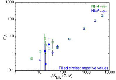
Figure 3: Lattice computations of the ratio $m_{3}$ shape with two different cutoffs ($N_{t}=4$ and 6). The two computations agree well with each other at $\sqrt{S}$ of about 50 GeV and higher. Below this the disagreement is due to cutoff effects in the location of the critical point.

If the theory were an ad-hoc model, one would not ask too much of it. However, when it is a first-principles method of computation in field theory one does need to examine systematic effects in various ways. Even in the comparison of perturbative QCD with collider data such questions are sometimes asked and occasionally the answers show the need for further work. For lattice thermodynamics the sources of systematic errors were enumerated in nt4 ; the main as-yet unquantified effect is of removing the lattice cutoff, i.e., the rate of approach to the continuum limit.

An exploration of this systematic effect shape is shown in Figure 3. The result of a computation of $m_{3}$ with two different lattice spacings is shown. The predictions for $\sqrt{S}>50$ GeV are clearly within control. There is less control at present at smaller lattice spacings. This can be traced to remaining lattice cutoff effects on the position of the critical point, which can be improved with further work on the lattice. This depends now largely on the computational power one can bring to the problem.

III.2 Experimental systematics

The most obvious systematic errors one must control in experiments is due to the fact that one is trying to apply the results of grand canonical thermodynamics to the data. One must then make sure that the experimental situation is close enough to local thermodynamic equilibrium: that the system is close to chemical equilibrium, that diffusive and advective phenomena are in balance, and that the part of the system under observation is neither too small nor too large. We will examine these questions in turn.

Geometric acceptance cuts in experiments, such as those on centrality, the pseudorapidity and azimuthal angle, serve to define the volume of the fireball which is observed, $V_{ob}$. If this volume is comparable to the full volume of the fireball, $V_{fb}$, then conserved quantities carry only initial state information. Fluctuations can still be observed, but they tell us about initial state fluctuations. These studies are of great interest because they can be correlated with other probes of the initial state kodama . However, none of the dedicated heavy-ion experiments have the acceptance to be able to do this. On the other hand the LHC detectors ALEPH and CMS with their near $4\pi$ coverage can easily be used to study initial state fluctuations of conserved quantities.

It is necessary to have $V_{ob}\ll V_{fb}$ in order for the unobserved part of the fireball to act as a reservoir of energy and particles so that thermodynamics in the grand canonical ensemble can be applied. Systematic corrections in powers of $V_{ob}/V_{fb}$ can be worked out koch . Another necessary condition is that the scale of observation should be much larger than the microscopic length scale in the fireball. For fluctuations of baryon number, the appropriate microscopic length scale to examine is the longest static correlation length of the baryon quantum number. The inverse of this correlation length is called the nucleon screening mass, ${\cal M}_{N}$. So, the condition that is usually required is ${\cal M}_{N}^{3}V_{ob}\gg 1$. At the critical point, where the divergence of $\chi^{(2)}$ implies the divergence of ${\cal M}_{N}$, the inequality does not hold, and QCD thermodynamics is not expected to describe the fluctuations berdnikov .

When the inequlity is valid, the observed volume contains many independently fluctuating volumes. As a result the shape of the distribution of fluctuations tends to a Gaussian; this is an application of the central limit theorem of statistics. The classic theory of fluctuations landau relate the mean and variance of the distribution to quantities such as $\chi^{(1)}$ and $\chi{(2)}$. Systematic corrections in powers of ${\cal M}_{N}^{3}V_{ob}$ relate higher cumulants to the NLS and lead to the study of observables such as those in eq. (3). The analysis of experimental data which was described in earlier sections is therefore part of the systematic theory of finite volume effects.

There is another length scale which needs to be investigated. If the total number of baryons and anti-baryons seen in a given event is $B_{+}=B+\overline{B}$, then the volume per detected baryon in that event is $V_{ob}/B_{+}=\zeta^{3}$. The distribution of $\zeta$ is of some interest in understanding thermalization. Extreme values of $\zeta$ are rare events in a thermal ensemble. If these appear more frequently than in a thermal ensemble, then that implies that initial random fluctuations in baryon number have not had time to equilibrate by diffusion. Such events would strongly influence tails of the event-to-event distribution of the net baryon number, and can distort measurements of the higher cumulants. Therefore, a study of high-order cumulants and their comparison with lattice predictions is of interest in understanding the speed of approach to equilibrium. It would be of special interest to divide the data sample into bins of $\zeta\leq 1$ or $\zeta>1$ or $\zeta\gg 1$, and compare the cumulants in different bins.

The competing dynamics of diffusion and flow create other length scales in the plasma bhalerao . If the expansion rate is small enough then fluctuations are evened out by diffusion. However, if the expansion rate is larger, then at some scale fluctuations are frozen into the fluid. Which of these actually occurs is discriminated by a dimensionless number called Peclet’s number—

$${\rm Pe}=\frac{\ell v}{\cal D},$$ (10)

where $\ell$ is the length scale of interest, $v$ is the flow velocity and $\cal D$ is the diffusion constant. When ${\rm Pe}\ll 1$ diffusion dominates and for ${\rm Pe}\gg 1$ baryon number is passively transported by the flow. As a result fluctuations freeze out when ${\rm Pe}\simeq 1$. Using the fact that ${\cal D}\simeq c_{s}/{\cal M}_{N}$, where $c_{s}$ is the speed of sound, we find that ${\rm Pe}=M\ell{\cal M}_{N}$, where $M$ is the Mach number. The freezeout scale for fluctuations, $\ell_{fo}$, is therefore

$$\ell_{fo}{\cal M}_{N}\simeq\frac{1}{M}.$$ (11)

If the observations see near-equilibrium fluctuations, then clearly one must have $\ell_{fo}\leq\sqrt[3]{V}_{ob}$. This implies that $V_{ob}{\cal M}_{N}^{3}\geq 1/M^{3}$. Since there is no evidence for shock waves in the fireball, one can assume that $M<1$, and therefore the observed volumes are sufficiently large for the usual finite size scaling theory to work.

Chemical freezeout occurs when various reaction rates become slower than the expansion rate. Most strong interaction cross sections are of very similar magnitude, so treating them as having a common freezeout parameter is expected to be a reasonable approximation. The fact that a model, such as the HRGM, which is based on this assumption works as a good description of the fireball is then not surprising.

It was recently pointed out asakawa that the isospin changing reaction, $p\leftrightarrow n$ which goes through the nearly resonant $\Delta$ channel has a very small energy denominator and therefore is relevant even after the chemical freezeout observed through fitted yields. This is an interesting observation since it can change the $n/p$ ratio from its thermal value. Since neutrons are uncharged and therefore unobservable, estimates of baryon fluctuations are based on the assumption that proton and neutron fluctuations are identical within errors. This was checked through event generators in star . It would be useful to check how strongly the proposal of asakawa affects event-generator estimates for proton fluctuations.

IV Summary

The observed agreement star of lattice predictions and experimental observations of fluctuations have many consequences. Among them are the possibilities of extracting measures of $T_{c}$ or freezeout conditions from a comparison of data and thermodynamic predictions from lattice computations shape . Interestingly, it also seems possible to extract the location of the critical point indirectly from an analysis of fluctuations observed at the highest energies in RHIC and LHC (see section II.2 and Figure 2).

There are indications of good control over systematic effects in lattice computations (see Figure 3 and the surrounding discussion), and future work will settle this. Some systematic errors on experiments have been dealt with in detail before; others are discussed here. The fluctuation observations of eq. (3) are finite size scaling quantities which take into account the effects of finite $V_{ob}{\cal M}_{N}^{3}$. Methods which take into account non-vanishing $V_{ob}/V_{fb}$ have been discussed recently koch . When $V_{ob}/V_{fb}\simeq 1$ then one has a “persistence of memory effect” which allows the study of initial state fluctuations in baryon number. The effect of fluctuations in volume per baryon may affect high moments, but are amenable to experimental investigation. The competing effects of flow and diffusion give rise to a “Peclet length scale” bhalerao which controls the time at which fluctuations at the scale of $V_{ob}$ freeze out. Hydrodynamic computations can give more details of this process in future. Slow isospin changing reactions asakawa have been noticed recently and their effects need to be understood.

In summary, the study of fluctuations has become very interesting as it emerges that there is more to understand and much to gain by doing so.

References

- (1) S. Gupta, PoS, CPOD2009 (2009) 25.
- (2) R. V. Gavai and S. Gupta, Phys. Lett. B 696 (2011) 459.
- (3) M. M. Aggarwal et al., (STAR Collaboration) Phys. Rev. Lett. 105 (2010) 022302.
- (4) R. V. Gavai and S. Gupta, Phys. Rev. D 68 (2003) 034506.
- (5) S. Gottlieb et al., Phys. Rev. D 38 (1988) 2888.
- (6) R. V. Gavai and S. Gupta, Phys. Rev. D 78 (2008) 114503.
- (7) Y. Aoki et al., Phys. Lett. B 643 (2006) 46.
- (8) H. Oeschler et al., PoS, CPOD2009 (2009) 32.
- (9) S. Gupta, X.-F. Luo, B. Mohanty, H.-G. Ritter and N. Xu, Science, 332 (2011) 1525.
- (10) F. Karsch, these proceedings.
-
(11)
B. Berdnikov and K. Rajagopal, Phys. Rev. D 61 (2000) 105017;
M. A. Stephanov, Phys. Rev. Lett. 102 (2009) 032301. - (12) R. V. Gavai and S. Gupta, Phys. Rev. D 71 (2005) 114014.
- (13) R. Andrade et al., Phys. Rev. Lett. 97 (2006) 203302.
- (14) V. Koch, these proceedings.
- (15) L. D. Landau and E. M. Lifshitz, Statistical Physics Part 1, (Elsevier, New Delhi, 2005)
- (16) R. S. Bhalerao and S. Gupta, Phys. Rev. C 79 (2009) 064901.
- (17) M. Kitazawa and M. Asakawa, arXiv:1107.2755.