Chaotic Method for Generating $q$-Gaussian Random Variables

Abstract

This study proposes a pseudo random number generator of $q$-Gaussian random variables for a range of $q$ values, $-\infty<q<3$, based on deterministic chaotic map dynamics. Our method consists of chaotic maps on the unit circle and map dynamics based on the piecewise linear map. We perform the $q$-Gaussian random number generator for several values of $q$ and conduct both Kolmogorov-Smirnov (KS) and Anderson-Darling (AD) tests. The $q$-Gaussian samples generated by our proposed method pass the KS test at more than 5% significance level for values of $q$ ranging from -1.0 to 2.7, while they pass the AD test at more than 5% significance level for $q$ ranging from -1 to 2.4.

I Introduction

The $q$-Gaussian distributions have been studied in a wide variety of fields from natural sciences to social sciences. They have been applied in thermodynamics, biology, economics, and quantum mechanics. The generating mechanism is still an open question, but several mechanisms that have been shown to produce $q$-Gaussian distributions are known, such as multiplicative noise, weakly chaotic dynamics, correlated anomalous diffusion, preferential growth of networks, and asymptotically scale-invariant correlations [1]. In the heavy-tail domain ($1<q<3$), the $q$-Gaussian distribution is equivalent to the Student’s $t$-distribution.

In the context of finance, the $q$-Gaussian distribution ($1<q<3$) is referred to as a Student’s $t$ distribution [2]. This is commonly used in finance and risk management, particularly to model conditional asset returns of which the tails are wider than those of normal distribution. The distribution is also known as Pearson Type-II (for compact support ($q<1$) and Type VII (infinite support ($q\geq 1$) [3]. For example, Bollerslev used the Student’s $t$ to model the distribution of the foreign exchange rate returns [4]. Bening and Korolev provide an instance where the distribution is appropriate as a model, i.e. the case of random sample sizes [5]. Vignat and Plastino obtained similar results [6]. Other work attempts to show the $q$-Gaussian distribution as an attractor in the context of dependent systems [7]. Moreover, Umarov et al. consider a $q$-extension of $\alpha$-stable Lévy distribution [8].

More recently, $q$-Gaussian distributions have been derived from the maximization of non-extensive entropy [1] and studied in the context of the generalization of Gauss’ Law of Errors [9]. $q$-Gaussian distributions can be derived from an infinite normal mixture with an inverse gamma distribution. This concept is known as superstatistics in non-equilibrium thermodynamics [10]. $q$-Gaussian distributions also appear as unconditional distributions of multiplicative stochastic differential equations [11].

Recently, the generalized Box-Muller method (GBMM) was proposed by Thisleton et al. [13]. Their method uses transformation including the $q$-logarithmic, sine, and cosine functions in terms of uniform random variables. Here, based on the ergodic theory [14] of dynamical systems, we propose a family of chaotic maps with an ergodic invariant measure given by $q$-Gaussian density. Ulam and von Neumann considered the logistic map $X_{n+1}=4X_{n}(1-X_{n})$ in the late 1940s, and found its randomness [15]. One of the authors (K. Umeno) proposed chaotic mechanism to generate power-law random variables [16]. This method can generate power-law random variables in the Lévy stable regime from the superposition of the random variables. One of the authors (A.-H. Sato) also proposed multiplicative random processes to generate power-law random variables [17]. Currently, we can use the map dynamics to design random sequences with an explicit ergodic invariant measure more precisely [18, 19].

In this article, we propose a method to generate $q$-Gaussian random variables based on deterministic map dynamics. Our method is based on ergodic transformations on the unit circle and a map composed of the piecewise linear map with both the $q$-exponential and $q$-logarithmic function. This method is a direct method different from Ref. [13, 16] and can generate $q$-Gaussian random variables for $-\infty<q<3$ including infinite variance and infinite mean regimes. We generate $q$-Gaussian random variables for several cases of $q$, and conduct statistical testing by means of analytical cumulative distribution functions.

II Review of the generalized Box-Muller Method

The zero-mean normal $q$-Gaussian distribution parameterized by $q$ is described as

$$g(x;q)=\left\{\begin{array}[]{ll}\frac{1}{B\Bigl{(}\frac{2-q}{1-q},\frac{1}{2}\Bigr{)}}\Bigl{(}\frac{1-q}{3-q}\Bigr{)}^{\frac{1}{2}}\Bigl{(}1{\color[rgb]{0,0,0}-\frac{1-q}{3-q}}x^{2}\Bigr{)}^{\frac{1}{1-q}}&(q<1)\\ \frac{1}{\sqrt{2\pi}}\exp\Bigl{(}-\frac{x^{2}}{2}\Bigr{)}&(q=1)\\ \frac{1}{B\Bigl{(}\frac{1}{1-{q}}-\frac{1}{2},\frac{1}{2}\Bigr{)}}\Bigl{(}\frac{{q}-1}{3-{q}}\Bigr{)}^{\frac{1}{2}}\Bigl{(}1{\color[rgb]{0,0,0}+\frac{q-1}{3-q}}x^{2}\Bigr{)}^{\frac{1}{1-q}}&(1<q<3)\end{array}\right.,$$ (1)

where $B(a,b)$ is the beta function, which is defined as

$$B(a,b)=\int_{0}^{1}t^{a-1}(1-t)^{b-1}\mbox{d}t.$$ (2)

For $q<1$ symmetric distributions with compact support ranging from $-\sqrt{\frac{2}{1-q}}$ to $\sqrt{\frac{2}{1-q}}$ appear. Specifically, the normalized Wigner distribution is obtained at $q=-1$. In the case of $1<q<3$, Equation 1 has heavy-tails and $g(x;q)\approx const.|x|^{\nu-1}$, where $\nu=(3-q)/(q-1)>0$ is related to the degree of freedom of the Student’s $t$-distribution. $\nu$ is coincident with the tail index of the complementary cumulative distribution of $g(x;q)$. This also gives an existence condition in the heavy-tail regime of the $q$-Gaussian distribution.

Firstly, let us start our discussion from the GBMM proposed by Thistleton et al. [13]. To introduce their method to generate $q$-Gaussian random variable, we define a $q$-analog of both exponential and logarithmic function.

Definition 1. Suppose the one-dimensional ordinary differential equation

$$\frac{\mbox{d}h}{\mbox{d}w}=h^{q},\quad h(0)=1.$$ (3)

The solution is given as

$$h(w)=\left\{\begin{array}[]{ll}\Bigl{(}1+(1-q)w\Bigr{)}^{\frac{1}{1-q}}&1+(1-q)w>0\\ 0&\mbox{elsewhere}\\ \end{array}\right..$$ (4)

We call the solution $h(w)$ $q$-exponential function. Obviously, one has

$$\lim_{q\rightarrow 1}\Bigl{(}1+(1-q)w\Bigr{)}^{\frac{1}{1-q}}=e^{w}.$$ (5)

Definition 2. We define the inverse function of Equation 4

$$\ln_{q}(w)=\frac{w^{1-q}-1}{1-q}\quad(w>0),$$ (6)

which we call the $q$-logarithmic function. Clearly, we get

$$\lim_{q\rightarrow 1}\frac{w^{1-q}-1}{1-q}=\ln w.$$ (7)

Definition 3. The GBMM [13] is given by transformations from i.i.d. uniform random variables $u_{1}$ and $u_{2}$ ranging from 0 to 1.

$$\left\{\begin{array}[]{lll}x&=&\sqrt{-2\ln_{q}(u_{1})}\cos(2\pi u_{2})\\ y&=&\sqrt{-2\ln_{q}(u_{1})}\sin(2\pi u_{2})\end{array}\right..$$ (8)

Proposition 1. The joint probability density of $x$ and $y$ in Equation 8, is given by

$$p_{X,Y}(x,y)=\frac{1}{2\pi}\exp_{2-1/q}\Bigl{(}-\frac{q}{2}(x^{2}+y^{2})\Bigr{)}.$$ (9)

Proof of Proposition 1. From Equation 8, we obtain

$$p_{U_{1}}(u_{1})p_{U_{2}}(u_{2}) = p_{X,Y}(x,y)\Bigl{|}\frac{\partial(x,y)}{\partial(u_{1},u_{2})}\Bigr{|}$$

$$1 = 2\pi p_{X,Y}(x,y)u_{1}^{-q}$$

$$p_{X,Y}(x,y) = \frac{1}{2\pi}\Bigl{[}\exp_{q}\bigl{(}-\frac{1}{2}(x^{2}+y^{2})\bigr{)}\Bigr{]}^{q}$$ (10)

$$= \frac{1}{2\pi}\exp_{2-1/q}\Bigl{(}-\frac{q}{2}(x^{2}+y^{2})\Bigr{)},$$

where we used the equality

$$\bigl{(}\exp_{q}(x)\bigr{)}^{q}=\bigl{(}1+(1-q)x\bigr{)}^{\frac{q}{1-q}}=\exp_{2-1/q}(qx).$$ (11)

Note that Equation 10 is recognized as a two-dimensional $q$-normal distribution,

$$p_{X,Y}(x,y)=\frac{1}{2\pi}\exp_{r}\Bigl{(}-\frac{1}{2+D(1-r)}(x^{2}+y^{2})\Bigr{)},\\$$ (12)

where $r=2-1/q$ and $D=2$. This is properly parameterized with each marginal $q$-variance equal to one.

Proposition 2. The marginal distribution of $x$ is given by

$$p_{X}(x)=\left\{\begin{array}[]{ll}\frac{1}{B\Bigl{(}\frac{2-q^{\prime}}{1-q^{\prime}},\frac{1}{2}\Bigr{)}}\Bigl{(}\frac{1-q^{\prime}}{3-q^{\prime}}\Bigr{)}^{\frac{1}{2}}\Bigl{[}1-\frac{1-q^{\prime}}{3-q^{\prime}}x^{2}\Bigr{]}^{\frac{1}{1-q^{\prime}}}&|x|\leq\sqrt{\frac{3-q^{\prime}}{1-q^{\prime}}}\quad(q^{\prime}<1)\\ \frac{1}{\sqrt{2\pi}}\exp\Bigl{(}-\frac{x^{2}}{2}\Bigr{)}&(q=q^{\prime}=1)\\ \frac{1}{B\Bigl{(}\frac{1}{1-{q^{\prime}}}-\frac{1}{2},\frac{1}{2}\Bigr{)}}\Bigl{(}\frac{{q^{\prime}}-1}{3-{q^{\prime}}}\Bigr{)}^{\frac{1}{2}}\Bigl{[}1+\frac{q^{\prime}-1}{3-q^{\prime}}x^{2}\Bigr{]}^{\frac{1}{1-q^{\prime}}}&(1<q^{\prime}<3)\end{array}\right.$$ (16)

where $q^{\prime}=(3q-1)/(q+1)$. Hence, $x$ in Equation 8 gives a $q^{\prime}$-Gaussian random variable.

Proof of Proposition 2. Integrating Equation 9 in terms of $y$, we obtain Equation 16. In the case of $q=1$, we obviously obtain

$$p_{X}(x) = \int_{-\infty}^{\infty}p_{X,Y}(x,y)dy$$ (17)

$$= \frac{1}{2\pi}\int_{-\infty}^{\infty}\exp\Bigl{(}-\frac{1}{2}(x^{2}+y^{2})\Bigr{)}\mbox{d}y$$

$$= \frac{1}{\sqrt{2\pi}}\exp\Bigl{(}-\frac{x^{2}}{2}\Bigr{)}.$$

In the case of $1<q<3$, we have

$$p_{X}(x) = \int_{-\infty}^{\infty}p_{X,Y}(x,y)dy$$ (18)

$$= \frac{1}{2\pi}\int_{-\infty}^{\infty}\exp_{2-1/q}\Bigl{(}-\frac{q}{2}(x^{2}+y^{2})\Bigr{)}\mbox{d}y$$

$$= \frac{1}{2\pi}\int_{-\infty}^{\infty}\Bigl{(}1-\frac{1-q}{2}(x^{2}+y^{2})\Bigr{)}^{\frac{q}{1-q}}\mbox{d}y$$

$$= \frac{1}{\pi}\int_{0}^{\infty}\Bigl{(}1-\frac{1-q}{2}(x^{2}+y^{2})\Bigr{)}^{\frac{q}{1-q}}\mbox{d}y$$

$$\Bigl{(}\zeta=1+\frac{q-1}{2}x^{2}\Bigr{)}$$

$$= \frac{1}{\pi}\zeta^{\frac{q}{1-q}}\int_{0}^{\infty}\Bigl{(}1+\frac{q-1}{2\zeta}y^{2}\Bigr{)}^{\frac{q}{1-q}}\mbox{d}y$$

$$\Bigl{(}t=\frac{1}{\frac{q-1}{2\zeta}y^{2}+1}\Bigr{)}$$

$$= \frac{1}{\pi\sqrt{2(q-1)}}\zeta^{\frac{q}{1-q}+\frac{1}{2}}\int_{0}^{1}t^{\frac{q}{q-1}-\frac{3}{2}}(1-t)^{-\frac{1}{2}}\mbox{d}t$$

$$= \frac{1}{\pi\sqrt{2(q-1)}}B\Bigl{(}\frac{q}{q-1}-\frac{1}{2},\frac{1}{2}\Bigr{)}\Bigl{(}1+\frac{q-1}{2}x^{2}\Bigr{)}^{-\frac{q+1}{2(q-1)}}.$$

Using the equality among beta function and gamma functions

$$B(a,b)=\frac{\Gamma(a)\Gamma(b)}{\Gamma(a+b)},$$ (19)

where the gamma function is defined as

$$\Gamma(a)=\int_{0}^{\infty}t^{a-1}e^{-t}\mbox{d}t,$$ (20)

and $\pi=\Gamma(\frac{1}{2})^{2}$,

$$\frac{B\bigl{(}\frac{q}{q-1}-\frac{1}{2},\frac{1}{2}\bigr{)}}{\pi}=\frac{\Gamma(\frac{q}{q-1}-\frac{1}{2})\Gamma(\frac{1}{2})}{\Gamma(\frac{1}{2})^{2}\Gamma(\frac{q}{q-1})}=\frac{\Gamma(\frac{q}{q-1}-\frac{1}{2})}{\Gamma(\frac{1}{2})\Gamma(\frac{q}{q-1})}.$$

Since we have $\Gamma(\frac{q}{q-1})=(\frac{q}{q-1}-1)\Gamma(\frac{q}{q-1}-1)=\frac{1}{q-1}\Gamma(\frac{q}{q-1}-1)$, we get

$$\frac{B\bigl{(}\frac{q}{q-1}-\frac{1}{2},\frac{1}{2}\bigr{)}}{\pi}=\frac{(q-1)\Gamma(\frac{q}{q-1}-\frac{1}{2})}{\Gamma(\frac{1}{2})\Gamma(\frac{q}{q-1}-1)}=\frac{q-1}{B\bigl{(}\frac{q}{q-1}-1,\frac{1}{2}\bigr{)}}.$$

Therefore, Equation 18 can be rewritten as

$$p_{X}(x)=\frac{1}{B(\frac{q}{q-1}-1,\frac{1}{2})}\Bigl{(}\frac{q-1}{2}\Bigr{)}^{\frac{1}{2}}\Bigl{(}1+\frac{q-1}{2}x^{2}\Bigr{)}^{-\frac{q+1}{2(q-1)}}.$$ (21)

Setting $q=\frac{q^{\prime}+1}{3-q^{\prime}}$, we obtain

$$p_{X}(x)=\frac{1}{B\Bigl{(}\frac{1}{1-{q^{\prime}}}-\frac{1}{2},\frac{1}{2}\Bigr{)}}\Bigl{(}\frac{{q^{\prime}}-1}{3-{q^{\prime}}}\Bigr{)}^{\frac{1}{2}}\Bigl{[}1+\frac{q^{\prime}-1}{3-q^{\prime}}x^{2}\Bigr{]}^{\frac{1}{1-q^{\prime}}}$$ (22)

In the case of $q<1$, we obtain the joint density $p_{X,Y}(x,y)$ has a compact support ranging from $-\sqrt{\frac{2}{1-q}x^{2}}$ to $\sqrt{\frac{2}{1-q}x^{2}}$.

$$p_{X}(x) = \int_{-\sqrt{\frac{2}{1-q}x^{2}}}^{\sqrt{\frac{2}{1-q}x^{2}}}p_{X,Y}(x,y)dy$$ (23)

$$= \frac{1}{2\pi}\int_{-\sqrt{\frac{2}{1-q}x^{2}}}^{\sqrt{\frac{2}{1-q}x^{2}}}\Bigl{(}1-\frac{1-q}{2}(x^{2}+y^{2})\Bigr{)}^{\frac{q}{1-q}}\mbox{d}y$$

$$= \frac{1}{\pi}\int_{0}^{\sqrt{\frac{2}{1-q}x^{2}}}\Bigl{(}1-\frac{1-q}{2}(x^{2}+y^{2})\Bigr{)}^{\frac{q}{1-q}}\mbox{d}y$$

$$\Bigl{(}\zeta=1-\frac{1-q}{2}x^{2}\Bigr{)}$$

$$= \frac{1}{\pi\sqrt{2(q-1)}}\zeta^{\frac{q}{1-q}+\frac{1}{2}}\int_{1}^{\infty}t^{\frac{q}{q-1}-\frac{3}{2}}(1-t)^{-\frac{1}{2}}\mbox{d}t$$

$$\Bigl{(}t=\frac{1}{s}\Bigr{)}$$

$$= -\frac{1}{\pi\sqrt{2(q-1)}}\zeta^{\frac{q}{1-q}+\frac{1}{2}}\int_{1}^{0}s^{\frac{q}{1-q}}(1-s)^{-\frac{1}{2}}\mbox{d}s$$

$$= \frac{1}{\pi\sqrt{2(q-1)}}B\Bigl{(}\frac{1}{1-q},\frac{1}{2}\Bigr{)}\Bigl{(}1-\frac{1-q}{2}x^{2}\Bigr{)}^{\frac{2q+1}{2(1-q)}}.$$

Similarly to the case of $1<q<3$ setting $q=\frac{q^{\prime}+1}{3-q^{\prime}}$, we obtain

$$p_{X}(x)=\frac{1}{B\Bigl{(}\frac{2-q^{\prime}}{1-q^{\prime}},\frac{1}{2}\Bigr{)}}\Bigl{(}\frac{1-q^{\prime}}{3-q^{\prime}}\Bigr{)}^{\frac{1}{2}}\Bigl{[}1-\frac{1-q^{\prime}}{3-q^{\prime}}x^{2}\Bigr{]}^{\frac{1}{1-q^{\prime}}},$$ (24)

where $|x|\leq\sqrt{\frac{3-q^{\prime}}{1-q^{\prime}}}$.

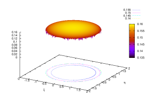
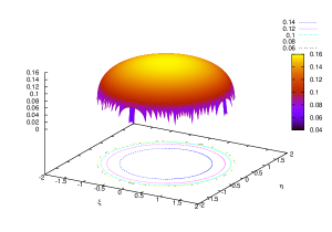
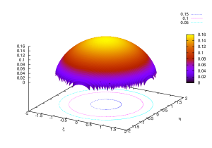
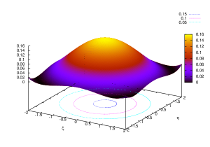
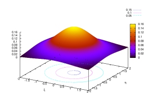
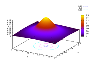
(a) (b) (c) (d) (e) (f) (g)

Figure 1: Three dimensional plots of joint density in terms of $\xi$ and $\eta$ for (a) $q^{\prime}=-0.9$, (b) $-0.4$, (c) $0.1$, (d) $0.6$, (e) $1.1$ (${\color[rgb]{0,0,0}\nu}=19$), (f) $1.6$ (${\color[rgb]{0,0,0}\nu}=2.33$), and (g) $2.1$ (${\color[rgb]{0,0,0}\nu}=0.818$).

Figure 1 shows the distribution of Equation 9 for several cases of $q$. The distribution is the spinning object. The marginal distribution in terms of $\xi$ is also equivalent to Equation 16.

III Map dynamics

Adler and Rivlin considered $P_{d}(w)=\cos d\theta$, where $w=\cos\theta$, $0\leq\theta\leq\pi$, defined by Chebyshev polynomial of degree $d$ [20], where $d$ is an integer. Clearly, $P_{d}(w)$ is permutable $P_{d_{1}}(P_{d_{2}}(w))=P_{d_{1}d_{2}}(w)$. They proved that for $d\geq 2$ the ergodic invariant measure of the map dynamics $w_{n+1}=P_{d}(w_{n})$ has an explicit density function invariant measure $\mu_{W}(w)=\frac{1}{\pi\sqrt{1-w^{2}}}$.

More generally, let us extend the Chebyshev polynomial to a two-dimensional case as [21].

Definition 4. $P_{d}(w)$ and $Q_{d}(w,v)$ are given as real and imaginary parts of binomial expansion,

$$(w+{\color[rgb]{0,0,0}i}v)^{d}=P_{d}(w)+{\color[rgb]{0,0,0}i}Q_{d}(w,v),$$ (25)

where the equality $w^{2}+v^{2}=1$ is necessary in order to obtain $P_{d}(w)$ from this expansion. Here, in this definition we used the Eular equality

$$(\exp({\color[rgb]{0,0,0}i}\theta))^{d}=\exp({\color[rgb]{0,0,0}i}d\theta)=\cos d\theta+{\color[rgb]{0,0,0}i}\sin d\theta.$$ (26)

This $P_{d}(w)$ is the Chebyshev polynomial of degree $d$. The first few polynomials are explicitly given by $P_{1}(w)=w$, $Q_{1}(w,v)=v$, $P_{2}(w)=2w^{2}-1$, $Q_{2}(w,v)=2wv$, $P_{3}(w)=4w^{3}-3w$, $Q_{3}(w,v)=v(4w^{2}-1)$, $P_{4}(w)=8w^{4}-8w^{2}+1$, $Q_{4}(w,v)=v(8w^{3}-4w)$, $P_{5}(w)=16w^{5}-20w^{3}+5w$, $Q_{5}(w,v)=v(16w^{4}-12w^{2}+1)$, $P_{6}(w)=32w^{6}-48w^{4}+18w^{2}-1$, $Q_{6}(w,v)=v(32w^{5}-32w^{3}+6w)$, $P_{7}(w)=64w^{7}-112w^{5}+56w^{3}-7w$, $Q_{7}(w,v)=v(64w^{6}-80w^{4}+24w^{2}-1)$, $P_{8}(w)=128w^{8}-256w^{6}+160w^{4}-32w^{2}+1$, and $Q_{8}(w,v)=v(128w^{7}-192w^{5}+80w^{3}-8w)$.

Definition 5. For $d\geq 2$, we define the map dynamics

$$w_{n+1} = P_{d}(w_{n})$$ (27)

$$v_{n+1} = Q_{d}(w_{n},v_{n})$$ (28)

on the unit circle $w_{n}^{2}+v_{n}^{2}=1$. The set of variables $(w_{n},v_{n})$ is uniformly distributed on the unit circle if we set an initial condition of $(w_{0},v_{0})$ on the unit circle. We set $v_{0}$ as an arbitrary value in $(0,1)$ and $w_{0}$ is given by $w_{0}=\pm\sqrt{1-v_{0}^{2}}$.

Lemma 1. The joint density of ergodic invariant measure for $w_{n+1}=P_{d}(w_{n})$ and $v_{n+1}=Q_{d}(w_{n},v_{n})$ follows

$$p_{W,V}(w,v)=\frac{\delta\bigl{(}\sqrt{w^{2}+v^{2}}-1\bigr{)}}{2\pi\sqrt{w^{2}+v^{2}}}.$$ (29)

Proof of Lemma 1. In addition to $P_{d}(w)=\cos d\theta$, we introduce $Q_{d}(w,v)=\sin d\theta$, where $w=\cos\theta$ and $v=\sin\theta$, $0\leq\theta\leq 2\pi$. From the equality given in Equation 26, the angular $\theta_{n}$ of $w_{n}+iv_{n}$ follows the map dynamics

$$\theta_{n+1}=d\theta_{n}\quad\mbox{mod}\quad 2\pi,$$ (30)

which is ergodic and has an ergodic density function [12]

$$p_{\Theta}(\theta)=\frac{1}{2\pi}\quad(0<\theta<2\pi).$$ (31)

Transforming the orthogonal coordinate $(w,v)$ into the polar coordinate $(a,\theta)$ by $w=a\cos\theta$ and $v=a\sin\theta$, we have $p_{A}(a)=\delta(a-1)$. Since ons has $a=\sqrt{w^{2}+v^{2}}$ $\frac{\partial w}{\partial a}=\cos\theta$, $\frac{\partial w}{\partial\theta}=-a\sin\theta$, $\frac{\partial v}{\partial a}=\sin\theta$, and $\frac{\partial v}{\partial\theta}=a\cos\theta$, the Jacobian matrix is expressed as

$$\Bigl{|}\frac{\partial(\theta,a)}{\partial(w,v)}\Bigr{|} = \left|\begin{array}[]{cc}\cos\theta&-a\sin\theta\\ \sin\theta&a\cos\theta\end{array}\right|^{-1}$$ (34)

$$= a^{-1}=\frac{1}{\sqrt{w^{2}+v^{2}}}.$$ (35)

Therefore, the joint density of the ergodic invariant measure of $w$ and $v$ can be described as

$$p_{W,V}(w,v) = p_{\Theta}(\theta)p_{A}(a)\Bigl{|}\frac{\partial(\theta,a)}{\partial(w,v)}\Bigr{|}$$ (36)

$$= \frac{\delta(\sqrt{w^{2}+v^{2}}-1)}{2\pi\sqrt{w^{2}+v^{2}}}.$$

Lemma 2. The density functions of ergodic invariant measure of Equation 27. and Equation 28, respectively, have the form:

$$\mu_{W}(w) = \frac{1}{\pi\sqrt{1-w^{2}}},$$ (37)

$$\mu_{V}(v) = \frac{1}{\pi\sqrt{1-v^{2}}}.$$ (38)

Proof of Lemma 2. From Equation 36 we can calculate $p_{W}(w)$ and $p_{V}(v)$ as the marginal distribution in terms of $w$ and $v$. Integrating Equation 36 with respect to $v$ and $w$, we respectively obtain

$$p_{W}(w) = \int_{-\infty}^{\infty}p_{WV}(w,v)\mbox{d}v$$ (39)

$$= \int_{-\infty}^{\infty}\frac{\delta\bigl{(}\sqrt{w^{2}+v^{2}}-1\bigr{)}}{2\pi\sqrt{w^{2}+v^{2}}}\mbox{d}v$$

$$= \frac{1}{\pi\sqrt{1-w^{2}}},$$

$$p_{V}(v) = \int_{-\infty}^{\infty}p_{WV}(w,v)\mbox{d}w$$ (40)

$$= \int_{-\infty}^{\infty}\frac{\delta\bigl{(}\sqrt{w^{2}+v^{2}}-1\bigr{)}}{2\pi\sqrt{w^{2}+v^{2}}}\mbox{d}w$$

$$= \frac{1}{\pi\sqrt{1-v^{2}}}.$$

Definition 6. As an alternative method for generating $q$-Gaussian random variables, we propose chaotic maps based on the following map dynamics:

$$\left\{\begin{array}[]{lll}w_{n+1}&=&{\color[rgb]{0,0,0}P_{d}(w_{n})}\\ v_{n+1}&=&{\color[rgb]{0,0,0}Q_{d}(w_{n},v_{n})}\\ z_{n+1}&=&f_{l,c}(z_{n})\end{array}\right.,$$ (41)

where

$$f_{l,c}(z) = g\circ{\color[rgb]{0,0,0}\underbrace{T_{l}\circ\cdots\circ T_{l}}_{c}}\circ g^{-1}(z),$$ (42)

$$w_{n}^{2}+v_{n}^{2} = 1,\qquad z_{n}>0$$ (43)

assuming

$$g(u) = \sqrt{-2\ln_{q}(u)},$$ (44)

$$g^{-1}(z) = \exp_{q}\Bigl{(}-\frac{z^{2}}{2}\Bigr{)},$$ (45)

where $T_{l}(u)$ is an $l$-th order piecewise linear map defined as

$$T_{l}(u)=\left\{\begin{array}[]{lc}\left\{\begin{array}[]{ll}lx&(0\leq u<1/l)\\ -lx+2&(1/l\leq<2/l)\\ \vdots&\\ lx-(l-1)&(1-1/l\leq x<1)\\ \end{array}\right.&(l:\mbox{odd})\\ \left\{\begin{array}[]{ll}lx&(0\leq u<1/l)\\ -lx+2&(1/l\leq<2/l)\\ \vdots&\\ -lx+l&(1-1/l\leq x<1)\\ \end{array}\right.&(l:\mbox{even})\end{array}\right.$$ (46)

For example, in the case of $l=2$, Equation 46 gives the tent map

$$T_{2}(u) = \left\{\begin{array}[]{ll}2u&(0\leq u<1/2)\\ -2u+2&(1/2\leq u<1)\end{array}\right.$$ (49)

$$= 1-|1-2u|.$$ (50)

In the case of $l=3$, Equation 46 is expressed as

$$T_{3}(u)=\left\{\begin{array}[]{ll}3u&(0\leq u<1/2)\\ -3u+2&(1/2\leq u<1)\\ 3u-2&(2/3\leq u<1)\end{array}\right.$$ (51)

The number of iteration $c$ is an integer greater than or equal to 1. The order $l$ of the piecewise linear map is an integer greater than or equal to 2. By using the product among $z_{n}$, $w_{n}$, and $v_{n}$,

$$\left\{\begin{array}[]{lll}\xi_{n}&=&z_{n}w_{n}\\ \eta_{n}&=&z_{n}v_{n}\\ \end{array}\right.,$$ (52)

we can also obtain two-dimensional deterministic dynamics. The random seed of this pseudo random generator is given by $(v_{0},z_{0})$, where we set $w_{0}$ as $w_{0}=\pm\sqrt{1-v_{0}^{2}}$.

Note that factor 2 in front of $q$-exponential function in Equation 50 should be replaced with a value both smaller than and close to 2, such as 1.99999, for the round error correction in the case of actual numerical computation.

Lemma 3. The density of ergodic invariant measure of $z_{n+1}=f_{l,c}(z_{n})$ follows the one-side distribution,

$$p_{Z}(z)=z\exp_{2-1/q}\Bigl{(}-\frac{q}{2}z^{2}\Bigr{)}\quad(z\geq 0).$$ (53)

Proof of Lemma 3. The density of the ergodic invariant measure [12] of the piecewise linear map

$$u_{n+1}={\color[rgb]{0,0,0}\underbrace{T_{l}\circ\cdots\circ T_{l}}_{c}}(u_{n}),$$ (54)

follows the uniform distribution $p_{U}(u)=1\quad(0<u<1)$ independently of $l$ and $c$. Since we obtain $\mbox{d}u/\mbox{d}z=u^{q}\sqrt{-2\ln_{q}(u)}$ from the transformation in Equation 44, we have

$$p_{Z}(z) = p_{U}(z)\Bigl{|}\frac{\mbox{d}u}{\mbox{d}z}\Bigr{|}$$ (55)

$$= z\Bigl{(}\exp_{q}(-z^{2}/2)\Bigr{)}^{q}$$

$$= z\exp_{2-1/q}\Bigl{(}-\frac{q}{2}z^{2}\Bigr{)}\quad(z\geq 0).$$

In this derivation, we used the equality introduced in Equation 11.

Theorem 1. The joint density $p_{\Xi,H}(\xi,\eta)$ of ergodic invariant measure of map dynamics Equation 52 is the $q$-Gaussian distribution which is the same as Equation 9 and given by

$$p_{\Xi,H}(\xi,\eta)=\frac{1}{2\pi}\exp_{2-1/q}\Bigl{(}-\frac{q}{2}(\xi^{2}+\eta^{2})\Bigr{)}.$$ (56)

Proof of Theorem 1. By using Equation 29 and Equation 53, the joint density $p_{\Xi,H}(\xi,\eta)$ of the ergodic invariant measure in terms of $\xi$ and $\eta$ is given as

$$p_{\Xi,H}(\xi,\eta) = \int_{0}^{\infty}p_{Z,W,V}(z,\xi/z,\eta/z)\Bigl{|}\frac{\partial(z,w,v)}{\partial(z,\xi,\eta)}\Bigr{|}\mbox{d}z$$ (57)

$$= \int_{0}^{\infty}p_{Z}(z)p_{W,V}(\xi/z,\eta/z)z^{-2}dz$$

$$= \int_{0}^{\infty}z^{-1}\exp_{2-1/q}\Bigl{(}-\frac{q}{2}z^{2}\Bigr{)}\frac{\delta\Bigl{(}\frac{1}{z}\sqrt{\xi^{2}+\eta^{2}}-1\Bigr{)}}{2\pi\sqrt{(\xi/z)^{2}+(\eta/z)^{2}}}\mbox{d}z$$

$$= \frac{1}{2\pi}\exp_{2-1/q}\Bigl{(}-\frac{q}{2}(\xi^{2}+\eta^{2})\Bigr{)}$$

Theorem 2. The marginal density of $\xi$ is a one-dimensional $q$-Gaussian distribution,

$$p_{\Xi}(\xi)=\left\{\begin{array}[]{ll}\frac{1}{B\Bigl{(}\frac{2-q^{\prime}}{1-q^{\prime}},\frac{1}{2}\Bigr{)}}\Bigl{(}\frac{1-q^{\prime}}{3-q^{\prime}}\Bigr{)}^{\frac{1}{2}}\Bigl{[}1-\frac{1-q^{\prime}}{3-q^{\prime}}\xi^{2}\Bigr{]}^{\frac{1}{1-q^{\prime}}}&|\xi|\leq\sqrt{\frac{3-q^{\prime}}{1-q^{\prime}}}\quad(q^{\prime}<1)\\ \frac{1}{\sqrt{2\pi}}\exp\Bigl{(}-\frac{\xi^{2}}{2}\Bigr{)}&(q=q^{\prime}=1)\\ \frac{1}{B\Bigl{(}\frac{1}{1-{q^{\prime}}}-\frac{1}{2},\frac{1}{2}\Bigr{)}}\Bigl{(}\frac{{q^{\prime}}-1}{3-{q^{\prime}}}\Bigr{)}^{\frac{1}{2}}\Bigl{[}1+\frac{q^{\prime}-1}{3-q^{\prime}}\xi^{2}\Bigr{]}^{\frac{1}{1-q^{\prime}}}&(1<q^{\prime}<3)\end{array}\right.,$$ (61)

where $q^{\prime}=(3q-1)/(q+1)$. Hence, sequences $\xi_{n}$ generated from the maps in Definition 1. are random numbers sampled from a $q^{\prime}$-Gaussian distribution, where $q^{\prime}=(3q-1)/(q+1)$.

Proof of Theorem. 2 From Proposition 2., the marginal distribution of $\xi$ is the same functional form as Equation 16.

IV Numerical simulation

Figure 2 shows sample paths for several values of $q^{\prime}$. As shown in these figures, they seem to be from a trapped random walk to Lévy walk as $q$ is increasing.

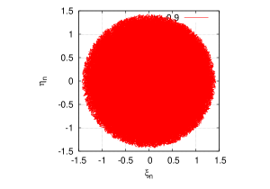
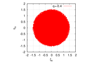
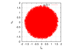
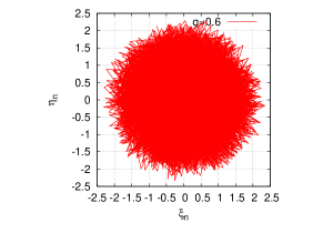
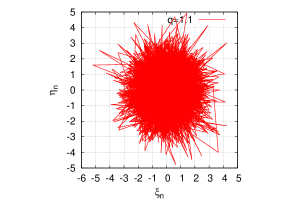
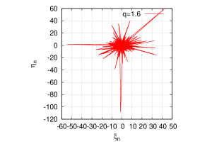
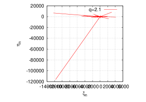
(a) (b) (c) (d) (e) (f) (g)

Figure 2: A sample path of the map dynamics at $d=8$, $l=2$, and $c=1$ for (a) $q^{\prime}=-0.9$, (b) $-0.4$, (c) $0.1$, (d) $0.6$, (e) $1.1$ (${\color[rgb]{0,0,0}\nu}=19$), (f) $1.6$ (${\color[rgb]{0,0,0}\nu}=2.33$), and (g) $2.1$ (${\color[rgb]{0,0,0}\nu}=0.818$).

Figure 3 shows the return maps between $z_{n+1}$ and $z_{n}$. They show the determinism of the proposed random number generator. The return map of $z_{n}$ at $l=2$ and $c=1$ shows the functional form of the map function introduced in Equation 42. $f_{2,1}(z)=0$ holds at $z=\sqrt{-2\ln_{q}(1/2)}$. Since one has

$$\frac{\mbox{d}f_{{\color[rgb]{0,0,0}2,1}}}{\mbox{d}z}=\left\{\begin{array}[]{l}-\frac{2^{1-q}\bigl{(}1-\exp_{q}(-\frac{z^{2}}{2})\bigr{)}^{-q}\bigl{(}1+(1-q)(-\frac{z^{2}}{2})\bigr{)}^{\frac{q}{1-q}}z}{\sqrt{-2\ln_{q}[2(1-\exp_{q}(-\frac{z^{2}}{2}))]}}\\ \qquad\qquad\qquad(z<\sqrt{-2\ln_{q}(1/2)})\\ \frac{2^{1-q}z}{\sqrt{-2\ln_{q}[2\exp_{q}(-\frac{z^{2}}{2})]}}\\ \qquad\qquad\qquad(z>\sqrt{-2\ln_{q}(1/2)})\\ \end{array}\right.,$$ (62)

the Lyapunov exponent of $z_{n}$, defined as

$$\lambda=\lim_{t\rightarrow\infty}\frac{1}{t}\sum_{n=0}^{t-1}\log\Bigl{|}f^{\prime}(z_{n})\Bigr{|}=\log 2=h_{KS},$$ (63)

is computable. Here, $h_{KS}$ is the Kolmogrov-Sinai entropy. The relation $\lambda=h_{KS}$ holds in one dimensional case by the Pesin identity. Independently of the initial conditions $(v_{0},z_{0})$ and the parameter $q$, it is numerically confirmed that the Lyapunov exponent $\lambda$ approaches $\log(2)$ at $l=2$ and $c=1$. This is consistent with the theoretical value of chaotic map, which is conjugate with a diffeomorphism $g$ for the tent map. More generally, the Lyapunov exponent $\lambda$ approaches to $c\log(l)$ in a general case of $f_{l,c}$. This iterated map is deterministic, however, the auto-correlation function of the productive variable $\xi=wz$,

$$C(m)=\lim_{t\rightarrow\infty}\frac{1}{t}\sum_{n=0}^{t-1}\xi_{n}\xi_{n+m}-\Bigl{(}\lim_{t\rightarrow\infty}\frac{1}{t}\sum_{n=0}^{t-1}\xi_{n}\Bigr{)}^{2},$$ (64)

decays 0 for $m\geq 1$ from the orthogonality of the Chebyshev polynomials. Obviously, the expectation value of $\xi$ is

$$\lim_{t\rightarrow\infty}\frac{1}{t}\sum_{n=0}^{t-1}\xi_{n}=\int_{-\infty}^{\infty}\xi p_{\Xi}(\xi)\mbox{d}\xi=0.$$ (65)

Since due to the independence of $w$ and $z$, we have

$$C(m) = \lim_{t\rightarrow\infty}\frac{1}{t}\sum_{n=0}^{t-1}w_{n}z_{n}\underbrace{P_{d}\circ\cdots\circ P_{d}}_{m}(w_{n})\underbrace{f_{l,c}\circ\cdots\circ f_{l,c}}_{m}(z_{n})$$ (66)

$$= \Bigl{(}\int_{-1}^{1}w\underbrace{P_{d}\circ\cdots\circ P_{d}}_{m}(w)\mu_{W}(w)\mbox{d}w\Bigr{)}$$

$$\times \Bigl{(}\int_{0}^{\infty}z\underbrace{f_{l,c}\circ\cdots\circ f_{l,c}}_{m}(z)p_{z}(z)\mbox{d}z\Bigr{)},$$

we obtain the auto-correlation of $\xi$ as

$$C(m)=\left\{\begin{array}[]{ll}\frac{1}{2}\delta_{1,2^{m}}B\Bigl{(}2,\frac{1}{1-q}\Bigr{)}&(q<1)\\ \frac{1}{2}\delta_{1,2^{m}}&(q=1)\\ \frac{1}{2}\delta_{1,2^{m}}B\Bigl{(}2,{\color[rgb]{0,0,0}\frac{3-q}{5-3q}}\Bigr{)}&(1<q<\frac{5}{3})\end{array}\right..$$ (67)

Note that $C(0)$ is not finite for $5/3<q<3$ since the variance of $q$-Gaussian distribution is not finite for $5/3<q<2$ and it is undefined for $2<q<3$. In this derivation, we used the permutability and the orthogonality of the Chebyshev polynomials,

$$\int_{-1}^{1}\underbrace{P_{{\color[rgb]{0,0,0}j}}\circ\cdots\circ P_{{\color[rgb]{0,0,0}j}}}_{n}(w)\underbrace{P_{{\color[rgb]{0,0,0}k}}\circ\cdots\circ P_{{\color[rgb]{0,0,0}k}}}_{m}(w)\mu_{W}(w)\mbox{d}w$$ (68)

$$= \int_{-1}^{1}P_{{\color[rgb]{0,0,0}j}^{n}}(w)P_{{\color[rgb]{0,0,0}k}^{m}}(w)\mu_{W}(w)\mbox{d}w$$

$$= \frac{1}{\pi}\int_{0}^{\pi}\cos({\color[rgb]{0,0,0}j}^{n}\theta)\cos({\color[rgb]{0,0,0}k}^{m}\theta)\mbox{d}\theta=\frac{1}{2}\delta_{{\color[rgb]{0,0,0}j}^{n},{\color[rgb]{0,0,0}k}^{m}}.$$

In the same way, it can be proved that the auto-correlation function of the productive variable $\eta=vz$ also decays 0 for $m\geq 1$.

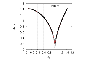
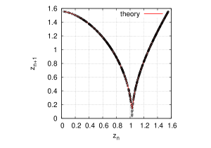
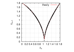
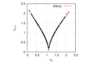
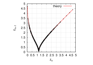
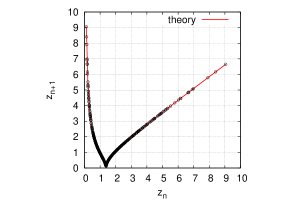
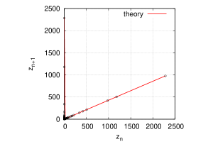
(a) (b) (c) (d) (e) (f) (g)

Figure 3: Return map between $z_{n}$ and $z_{n+1}$ for (a) $q^{\prime}=-0.9$, (b) $-0.4$, (c) $0.1$, (d) $0.6$, (e) $1.1$ (${\color[rgb]{0,0,0}\nu}=19$), (f) $1.6$ (${\color[rgb]{0,0,0}\nu}=2.33$), and (g) $2.1$ (${\color[rgb]{0,0,0}\nu}=0.818$). The solid curve represents $z_{n+1}=f_{2,1}(z_{n})$ for each value of $q=(q^{\prime}+1)/(3-q^{\prime})$.

The cumulative distribution of $\xi$ generated by Equation 41. Equation 42. and Equation 52, defined as

$$\mbox{Pr}(\Xi\leq\xi)=\int_{-\infty}^{\xi}p_{\Xi}(\xi^{\prime})\mbox{d}\xi^{\prime},$$ (69)

can be expressed as

$$\mbox{Pr}(\Xi\leq\xi)=\left\{\begin{array}[]{ll}\left\{\begin{array}[]{ll}1&\xi>\sqrt{\frac{3-q^{\prime}}{1-q^{\prime}}}\\ \frac{1}{2}\Bigl{[}1+\mbox{sign}(\xi)\beta\bigl{(}\frac{1-q^{\prime}}{3-q^{\prime}}\xi^{2};\frac{1}{2},\frac{2-q^{\prime}}{1-q^{\prime}}\bigr{)}\Bigr{]}&|\xi|\leq\sqrt{\frac{3-q^{\prime}}{1-q^{\prime}}}\\ 0&\xi<-\sqrt{\frac{3-q^{\prime}}{1-q^{\prime}}}\end{array}\right.&\mbox{for}\quad q<1\\ 1-\frac{1}{2}\mbox{erfc}\Bigl{(}\frac{\xi}{\sqrt{2}}\Bigr{)}&\mbox{for}\quad q=1\\ \frac{1}{2}\Bigl{[}1+\mbox{sign}(\xi)\beta\bigl{(}\frac{\frac{q^{\prime}-1}{3-q^{\prime}}\xi^{2}}{1+\frac{q^{\prime}-1}{(3-q^{\prime})}\xi^{2}};\frac{1}{2},\frac{1}{q^{\prime}-1}-\frac{1}{2}\bigr{)}\Bigr{]}&\mbox{for}\quad 1<q<3\end{array}\right.,\\$$

where $\beta(x;a,b)$ is the regularized incomplete beta function,

$$\beta(x;a,b)=\frac{1}{B(a,b)}\int_{0}^{x}t^{a-1}(1-t)^{b-1}\mbox{d}t,$$ (70)

and $\mbox{erfc}(x)$ is the complementary error function defined as

$$\mbox{erfc}(x)=\frac{2}{\sqrt{\pi}}\int_{x}^{\infty}e^{-t^{2}}\mbox{d}t.$$ (71)

We compare the cumulative distributions of $\xi_{n}$ obtained from Equation 41. Equation 42, and Equation 52 with Equation IV. Since we normally generate $q$-Gaussian random variables from the given $q^{\prime}$, for practical usage, we need the inverse relation between $q$ and $q^{\prime}$: $q=(q^{\prime}+1)/(3-q^{\prime})$. Figure 4 shows the empirical complementary cumulative distributions of $\xi$,

$$\mbox{Pr}(\Xi\geq\xi)=1-\mbox{Pr}(\Xi\leq\xi),$$ (72)

computed from 10,000 samples for $(w_{0},z_{0})=(0.1,1.0)$. Comparing the empirical distribution with the theoretical one, we found that they are very close for each parameter $q^{\prime}$.

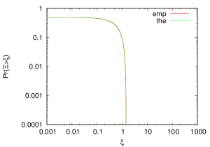
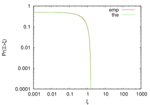
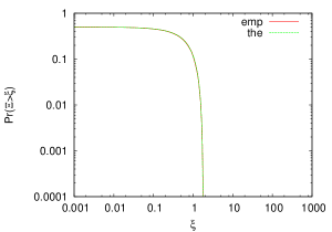
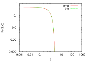
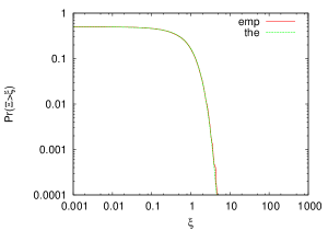
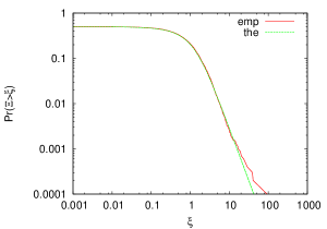
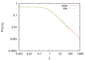
(a) (b) (c) (d) (e) (f) (g)

Figure 4: Complementary cumulative distribution functions of $\xi$ at $d=8$, $l=2$, and $c=1$ for (a) $q^{\prime}=-0.9$, (b) $-0.4$, (c) $0.1$, (d) $0.6$, (e) $1.1$ (${\color[rgb]{0,0,0}\nu}=19$), (f) $1.6$ (${\color[rgb]{0,0,0}\nu}=2.33$), and (g) $2.1$ (${\color[rgb]{0,0,0}\nu}=0.818$). Red curves represent empirical distributions, and green ones represent theoretical distributions.

TABLE I: The best KS and AD statistics obtained from 10,000 samples in 100 trials for several $q$ at $d=8$, $l=2$, and $c=1$. $p$-values of both KS and AD tests are shown.

$q$	${\color[rgb]{0,0,0}\nu}$	$p$-value (AD)	$p$-value (KS)
-1.0	-	0.996000	0.985991
-0.9	-	0.994000	0.974883
-0.8	-	0.997200	0.999401
-0.7	-	0.995800	0.996095
-0.6	-	0.995800	0.990724
-0.5	-	0.992200	0.994215
-0.4	-	0.992200	0.998253
-0.3	-	1.000000	0.998473
-0.2	-	0.995600	0.999262
-0.1	-	1.000000	0.994604
0.0	-	0.994400	0.988120
0.1	-	0.996000	0.986996
0.2	-	0.995800	0.998657
0.3	-	0.996600	0.972872
0.4	-	0.994800	0.979354
0.5	-	0.995000	0.980051
0.6	-	0.996600	0.993282
0.7	-	0.997200	0.996990
0.8	-	0.996000	0.984822
0.9	-	0.996000	0.999201
1.0	-	0.990400	0.998745
1.1	19	0.992000	0.997347
1.2	9	0.984400	0.963889
1.3	5.66	0.994400	0.983520
1.4	4	0.996400	0.995607
1.5	3	0.994400	0.997567
1.6	2.33	0.995000	0.999408
1.7	1.85	0.996200	0.990171
1.8	1.5	0.995600	0.994572
1.9	1.22	0.996800	0.984163
2.0	1	0.995800	0.995830
2.1	0.818	0.992000	0.995684
2.2	0.666	0.996000	0.982779
2.3	0.538	0.995800	0.993096
2.4	0.428	0.000000	0.875352
2.5	0.333	0.000000	0.995347
2.6	0.25	0.000000	0.994969
2.7	0.176	0.000000	0.007562
2.8	0.111	0.000000	0.000000
2.9	0.052	0.000000	0.000000

TABLE II: The best KS and AD statistics obtained from 10,000 samples in 100 trials for several $q$ at $d=6$, $l=2$, and $c=6$. $p$-values of both KS and AD tests are shown.

$q$	${\color[rgb]{0,0,0}\nu}$	$p$-value (AD)	$p$-value (KS)
-1.0	-	0.993600	0.998321
-0.9	-	0.994800	0.999067
-0.8	-	0.994400	0.997075
-0.7	-	0.996200	0.994040
-0.6	-	0.991600	0.992699
-0.5	-	0.994600	0.999246
-0.4	-	0.995000	0.973464
-0.3	-	0.995400	0.992854
-0.2	-	0.995600	0.983395
-0.1	-	0.994800	0.992643
0.0	-	0.997000	0.980508
0.1	-	0.995800	0.996620
0.2	-	0.996000	0.999265
0.3	-	0.996600	0.970387
0.4	-	0.996200	0.992929
0.5	-	0.996000	0.999219
0.6	-	0.992200	0.995459
0.7	-	0.996400	0.991304
0.8	-	0.994400	0.959594
0.9	-	0.995800	0.999786
1.0	-	0.993800	0.997754
1.1	19	0.996400	0.998304
1.2	9	0.979800	0.959894
1.3	5.66	0.99600	0.999363
1.4	4	0.995800	0.987967
1.5	3	0.994800	0.978924
1.6	2.33	0.995800	0.999754
1.7	1.85	0.996400	0.994942
1.8	1.5	0.995400	0.999325
1.9	1.22	0.997000	0.994694
2.0	1	0.996400	0.978461
2.1	0.818	0.988800	0.999509
2.2	0.666	0.996400	0.991371
2.3	0.538	0.996400	0.997778
2.4	0.428	0.000000	0.928166
2.5	0.333	0.000000	0.981747
2.6	0.25	0.000000	0.989397
2.7	0.176	0.000000	0.007562
2.8	0.111	0.000000	0.000000
2.9	0.052	0.000000	0.000000

We conducted the Kolmogorov-Smironov (KS) and the Anderson-Darling (AD) tests in order to verify whether the empirical distributions of sequences generated by our proposed method are convergent to the $q$-Gaussian distributions. It is known that Anderson–Darling test is suitable for checking the goodness-of-fit for heavy-tailed distributions [22]. Assuming $M$ samples of $\xi_{1},\ldots,\xi_{M}$, the test statistics are given as

$$Z=\sqrt{M}\max_{n}\Bigl{|}F_{M}(\xi_{n})-\mbox{Pr}(\Xi\geq\xi_{n})\Bigr{|}\sqrt{\psi\bigl{(}\mbox{Pr}(\Xi\geq\xi_{n})\bigr{)}},$$ (73)

where $F_{M}(\xi_{n})$ an empirical cumulative distribution function, and $\psi(u)$ is a weight function. In the case of $\psi(u)=1$, $Z$ gives a KS test statistic and in the case of $\psi(u)=\frac{1}{u(1-u)}$, $Z$ gives an AD test statistic.

Table I shows the best $p$-values of both KS and AD tests for several $q$ values at $d=8$, $l=2$, and $c=1$. The $p$-value of KS test is greater than 0.1 for $q<2.7$. Therefore, the null hypothesis that the sequences are not samples from the theoretical distribution is not rejected at more than 5% statistical significance for $q$ values from 1 to 2.6 in KS test. The degree of freedom $\nu$ goes to 0 as $q$ approaches 3. For $q>2.7$ (${\color[rgb]{0,0,0}\nu}<0.17$), both the proposed procedure and GBMM does not work since degree of freedom $\nu$ is very small. The $p$-value of AD test is greater than 0.1 for $q<2.4$. Since AD test is sensitive for tail events, the null hypothesis is not rejected from the value of $q$ smaller than KS test values. Table II shows the $p$-values of both KS and AD tests for several $q$ values at $d=6$, $l=2$, and $c=6$. The tendency of $p$-values is very similar to ones at $d=8$, $l=2$, and $c=1$. The KS test passes at more than 5% statistical significance for $q$ values ranging from -1 to 2.6 in KS test. The same is true for $-1\leq q<2.4$ in the case of AD test.

While GBMM [13] is based on transformation of uniform random variables, our proposed method here is purely mechanical generation of $q$-Gaussian distribution based on ergodic theory. Thus, no random number are not assumed for the generations of $q$-Gaussian distribution. Its implementation is very simple as shown in the example code in Appendix  A. Figures 6 ($d=8$, $l=2$, and $c=1$) and 5 ($d=6$, $l=2$, and $c=6$) show the best p-values of (a) KS test and (b) AD test obtained from 10,000 samples in 100 trials with the proposal and the GBMM for several $q$. The best $p$-values provided by the proposed method are same as ones by the GBMM for many cases.

(a) (b)

Figure 5: (a) The best $p$-values of both (a) KS and (b) AD tests obtained from 10,000 samples in 100 trials with our proposed and GBMM for several $q$ at $d=8$, $l=2$, and $c=1$.

(a) (b)

Figure 6: (a) The best $p$-values of both (a) KS and (b) AD tests obtained from 10,000 samples in 100 trials with our proposed and GBMM for several $q$ at $d=6$, $l=2$, and $c=6$.

V Conclusion

We proposed a pseudo random number generator of $q$-Gaussian random variables for a range of $q$ values, $-\infty<q<3$, based on deterministic map dynamics. Our method consists of ergodic transformation on the unit circle and map dynamics based on the piecewise linear map. We conducted both KS and AD tests for random number sequences generated by GBMM and our proposed chaotic method for several values of $q$. The $q$-Gaussian samples passed the KS test at the 5% significance level for $q<2.7$, and passed the AD test at the 5%significance level for $q<2.4$.

Appendix A Source code

We show a C source code for our proposed method for $d=8$, $l=2$, and $c=1$. The code is exhibited in order to demonstrate the algorithm, and is not optimal for speed. The algorithm is implemented in four functions. The first two functions compute $q$-exponential and $q$-logarithmic functions. The next function setseed_qnormal($v_{0}$, $z_{0}$) sets two random seeds $v_{0}$ and $z_{0}$, and qnormal($q$) calls the iterated map to generate $q$-Gauss random variables by our proposed method.

#include <stdio.h>
#include <math.h>
#include <stdlib.h>
#include <strings.h>
double qnormal_x,qnormal_y,qnormal_z;
double expq(double q, double w){
  if(q==1.0){
    return(exp(w));
  }
  else{
    return (expl(log(1.0+(1.0-q)*w)/(1.0-q)));
  }
}
double lnq(double q, double w){
  if(q==1.0){
    return(log(w));
  }
  else{
    return ((exp(log(w)*(1.0-q))-1.0)/(1.0-q));
  }
}
void setseed_qnormal(double v0, double z0){
  qnormal_x = sqrt(1-v0*v0);
  qnormal_y = v0;
  qnormal_z = z0;
}
double Q8(double w, double v){
  return(8*w*v*(((16.0*w*w-24.0)*w*w+10.0)*w*w-1.0));
}
double P8(double w){
  return((((128.0*w*w-256.0)*w*w+160.0)*w*w-32.0)*w*w+1.0);
}
double f(double z){
  return(1.0-fabs(1.0-1.99999*z));
}
void qnormal(double q){
  double qq;
  qnormal_y = Q8(qnormal_x,qnormal_y);
  qnormal_x = P8(qnormal_x);
  qq = (q+1.0)/(3.0-q);
  qnormal_z = f(expq(qq,-qnormal_z*qnormal_z*0.5));
  qnormal_z = sqrt(-2.0*lnq(qq,qnormal_z));
}
int main(int argc, char *argv[]){
  double q,v0,z0,eta,xi;
  int i;
  if(argc != 4){
     printf("%s q v0 z0\n",argv[0]);
     exit(0);
  }
  q = (double)atof(argv[1]);
  v0 = (double)atof(argv[2]);
  z0 = (double)atof(argv[3]);
  setseed_qnormal(v0,z0);
  for(i=0;i<10000;i++){
    qnormal(q);
    xi = qnormal_x*qnormal_z;
    eta = qnormal_y*qnormal_z;
    printf("%lf %lf\n",xi,eta);
  }
}