The variability of tidewater-glacier calving:
origin of event-size and interval distributions

Abstract

Calving activity at the termini of tidewater glaciers produces a wide range of iceberg sizes at irregular intervals. We present calving-event data obtained from continuous observations of the termini of two tidewater glaciers on Svalbard, and show that the distributions of event sizes and inter-event intervals can be reproduced by a simple calving model focusing on the mutual interplay between calving and the destabilization of the glacier terminus. The event-size distributions of both the field and the model data extend over several orders of magnitude and resemble power laws. The distributions of inter-event intervals are broad, but have a less pronounced tail. In the model, the width of the size distribution increases with the calving susceptibility of the glacier terminus, a parameter measuring the effect of calving on the stress in the local neighborhood of the calving region. Inter-event interval distributions, in contrast, are insensitive to the calving susceptibility. Above a critical susceptibility, small perturbations of the glacier result in ongoing self-sustained calving activity. The model suggests that the shape of the event-size distribution of a glacier is informative about its proximity to this transition point. Observations of rapid glacier retreats can be explained by supercritical self-sustained calving.

1 Introduction

Iceberg calving plays a key role in glacier dynamics, and hence in how tidewater glaciers and ice sheets respond to climate change, thereby impacting predictions of sea level rise in the future (????). So far, the mechanisms underlying the calving dynamics are only partly understood. To summarize the potential controls affecting iceberg calving, ? proposed the following classification: first-order controls determining the position of the glacier terminus, second-order controls responsible for the calving of individual icebergs, and third-order controls related to the calving of submarine icebergs. The first-order control on calving is the strain rate resulting from spatial variations in the glacier velocity, responsible for the opening of crevasses. Crevasse formation is reinforced by the presence of liquid water, either from surface melt or rain events. Second-order controls are processes weakening the glacier terminus and favoring fractures, like the presence of force imbalances at the glacier terminus resulting from the margin geometry, undercutting of ice and torque due to buoyancy. Third-order controls trigger submarine iceberg calving by processes like the formation of basal crevasses, tides and buoyancy.

The majority of previous studies describes calving by means of macroscopic variables such as the overall calving rate (calving speed), i.e. the total ice loss at the glacier terminus within rather long time intervals. Corresponding models (“calving laws”) relate the dynamics of the calving speed to parameters like the water depth (??), the height-above-buoyancy (???), the penetration of surface and basal crevasses arising from the longitudinal strain near the calving terminus and surface melt (???), and more general glacier characteristics such as the ice thickness, the thickness gradient, the strain rate, the mass-balance rate, and backward melting of the terminus (?).

So far, only few studies have been dedicated to a description of calving dynamics at the level of individual calving events. Continuous monitoring of individual events directly at the glacier terminus is challenging; consequently, data are sparse. Previous studies of the calving-event statistics were based on occasional or discontinuous observations of calving events (???), or on indirect measurements, e.g. event sizes obtained from icebergs floating in the sea (???) or from seismic activity (?). The available data indicate that event sizes are highly variable and broadly distributed (e.g. ??). However, distributions of event sizes obtained from floating icebergs in the sea are likely to be biased due to melting and disintegration (??). Seismic measurements can only detect large calving events reliably (?). In addition, estimating calving-event sizes (ice volume) from seismic-event magnitudes is problematic unless the relation between these two quantities is clearly established (e.g. through calibration by means of direct visual observations; see ?). Hence, the resulting size distributions may be biased. In principle, calving activity at the single-event scale could be monitored by means of repeat photography (?), laser scanning, or ground-based radar (?). So far, however, no such data have been published. Here, we present single-event data obtained from continuous visual observations directly at the termini of two tidewater glaciers on Svalbard. Our data confirm that both the sizes of individual calving events and the time intervals between consecutive events are broadly distributed.

So far, the mechanisms underlying this calving variability remain unknown. It is unclear whether it reflects variability in external conditions, e.g. temperature or tides, or whether it is generated by the internal calving dynamics itself. Fluctuations in external conditions can hardly be controlled in nature. Disentangling these two potential sources of variability therefore requires a model of the calving process. A description of the size and timing of individual calving events is beyond reach of the macroscopic continuum models focusing on the overall calving rate (see above). ?, ? and ? proposed models accounting for the discreteness of calving. In the model of ?, calving events are triggered when the terminus thickness decreases to some critical value. According to this model, the event sizes and inter-event intervals are fixed for constant model parameters. Variability in event sizes and intervals can only result from fluctuations (e.g. seasonal variations) in these parameters. ? describes the motion of the glacier terminus in one dimension as a stochastic process. In the study of ?, calving is modeled as a percolation process in a two-dimensional lattice representing a region close to the glacier terminus. In this model, microfractures are randomly and independently generated according to some cracking probability. Calving events occur whenever a section of ice is surrounded by a cluster of connected microfractures. In this model, calving in one region of the model glacier has no effect on the state of the rest of the glacier. Both the model of ? and that of ? are inherently stochastic. In our study, we propose an alternative calving model focusing on the mutual interplay between calving and the destabilization of the local neighborhood of the calving region. Although the calving dynamics of this model is fully deterministic, it generates broad distributions of event sizes and inter-event interval distributions which are consistent with the field data, even under stationary conditions.

Ultimately, breaking of ice, formation of fractures (crevasses) and, therefore, calving are consequences of internal ice stress (?). Several mechanisms contribute to the build-up of stress at the glacier terminus, e.g. glacier-velocity gradients, buoyancy, tides, or changes in the glacier-terminus geometry due to calving itself. The model proposed in this study describes the interplay between internal ice stress and calving as a positive-feedback loop: the glacier calves if the internal ice stress exceeds a critical value. The detachment of ice leads to an increase in stress in the neighborhood of the calving region, mainly due to a loss buttress, but also as a consequence of a reduction in ice burden pressure, increase in buoyancy and terminus acceleration. This increase in ice stress destabilizes the neighborhood of the calving region, i.e. increases the likelihood of calving. In our model, the calving-induced change in ice stress is captured by a parameter, the calving susceptibility. We show that the positive-feedback loop between calving and terminus destabilization alone is sufficient to explain the large variability of iceberg sizes and inter-event intervals observed in the field data. In the model, all other stress contributors are treated as “external stress” or described by parameters. Keeping these parameters constant enables us to study the glacier dynamics under (ideal) stationary conditions.

The paper is organized as follows: we first describe the acquisition of the field data, the calving model and the data analysis (Sec. 2). We then present the event-size and interval distributions obtained from the field data and show that they are reproduced by the calving model (Sec. 3.1). The model predicts a large variability in the calving process even under stationary external conditions. This is supported by the field data showing that the shape of the size and interval distributions is not affected by registered fluctuations in climatic conditions (Sec. 3.2). Next, we discuss a prediction of the model which may be of significance for judging the stability of a glacier: the model glacier exhibits a critical point at which it enters a regime of ongoing self-sustained calving (Sec. 3.3), a regime which may be related to observations of rapid glacier retreats. Finally, we demonstrate that the calving model is consistent with the field data in the sense that the size of future calving events is barely predictable from past events (Sec. 3.4). In the last section (Sec. 4), we summarize and discuss the consequences of our work, embed the results into the literature and point out limitations and possible extensions.

2 Methods

2.1 Acquisition of field data

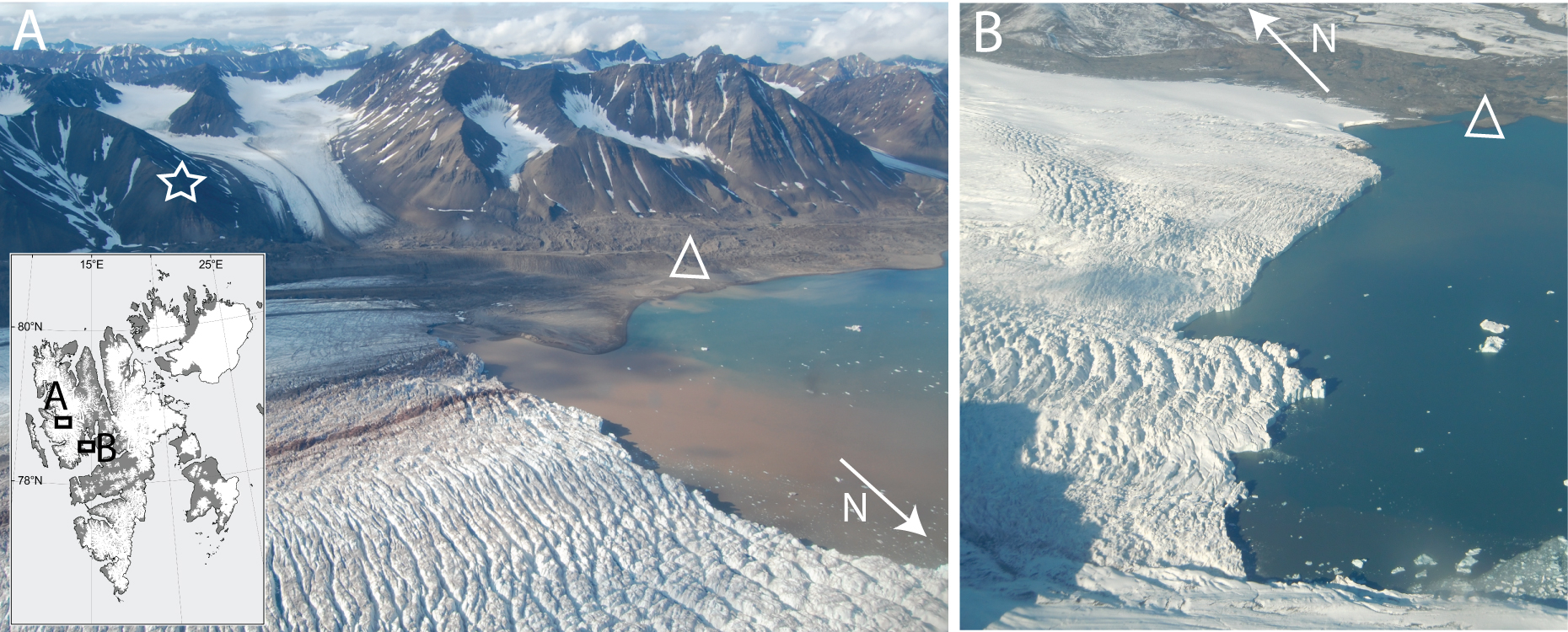
Study regions. Calving activity was monitored at two tidewater glaciers on Svalbard: Kronebreen and Sveabreen. Kronebreen is a grounded, polythermal tidewater glacier, located at $78^{o}53N$, $12^{o}30E$, approximately $14\,\text{km}$ south-east of Ny-Ålesund, western Spitsbergen (Fig. 1A). It is one of the fastest tidewater glaciers on Svalbard with an average terminus velocity between $2.5$ and $3.5\,\text{m}/\text{d}$ during the summer months (?). Calving activity was monitored over a 4- (August 26th, 2008, 19:00, to September 1st, 2008, 05:11, GMT) and a 12-day period (August 14th, 2009, 00:00, to August 26th, 2009, 16:00, GMT). At the end of August 2008, the terminal ice cliff had an elevation between $5$ and $60\,\text{m}$ above water level (?). About $90\text{\%}$ of the glacier terminus was visible from the observation camp, located approximately $1.5\,\text{km}$ west of the glacier terminus (Fig. 1, open white triangle). The second glacier, Sveabreen, is a $30\,\text{km}$ long, grounded tidewater glacier located at $78^{o}33N$, $14^{o}20E$, terminating in the northern part of Isfjorden (Fig. 1B). The observation of Sveabreen was part of a Youth Expedition program with 45 participants, lasting from July 17, 2010, 14:40, to July 21, 2010, 15:00 (GMT). The camp was located approximately $500-700\,\text{m}$ from the glacier terminus and offered an unobstructed view.

Figure 1: Aerial pictures of Kronebreen (A) and Sveabreen (B) taken in August 2009 and August 2010, respectively. Locations of the observation camps and the time-lapse camera are marked by triangles and the star, respectively. Inset: Map of Svalbard showing the location of the two glaciers.

Perceived event sizes and inter-event intervals. Calving activity was monitored by means of direct visual (and auditory) inspection of the glacier termini through human observers. At both observation sites, Kronebreen and Sveabreen, midnight sun lasts from April 18 to August 24. Hence, calving activity could be monitored continuously (day and night). Groups of 2–3 observers worked in alternate shifts. Note that, despite multiple observers, each calving event was registered only once. For each calving event, we registered the type (avalanche, block slump, column drop, column rotation, submarine event; see ??), location, time and perceived size. For the data analysis, we did not distinguish between different event types. Due to delays between the occurrence of events and the registration by the human observers, we assign a temporal precision of $\pm{}1$ minute to the inter-event intervals $\tau$, the time between two consecutive events. Following the semi-quantitative approach introduced by ?, we monitored the perceived size $\psi\in\{1,2,\ldots\}$ of each calving iceberg on an integer scale (?). The smallest observable events ($\psi=1$) correspond to icebergs with a volume of about $10\,\text{m}^{3}$, the largest ($\psi=11$) to more than $10^{5}\,\text{m}^{3}$ (collapse of about $1/5$th of the glacier terminus). During common observation periods, the perceived event sizes $\psi$ registered by different observers could be compared. Based on these data, the error (variability) in $\psi$ is estimated as $\pm{}1$.

Mapping perceived event sizes to iceberg volumes. The perceived iceberg sizes $\psi$ were mapped to the actual iceberg volumes $\mu$ by means of photogrammetry: repeat photographs were automatically taken at $3$-second intervals from a fixed location (star in Fig. 1) using Harbotronics time-lapse cameras (see ?, and references therein). In the resulting data, we identified $18$ calving events which were simultaneously registered by human observers. The approximate volume $\mu$ of each event was obtained from the estimated iceberg dimensions, and compared to the perceived size $\psi$ (see Fig. 2). The relation between $\mu$ and $\psi$ is well fit by a power law (dashed line in Fig. 2; correlation coefficient $c=0.68$ in double-logarithmic representation):

$$\mu=12.6.\psi^{3.87}.$$ (1)

Note that the empirical power-law model (1) is consistent with psychophysical findings (“Stevens’ power law”; ?). Using (1), we converted the perceived iceberg sizes $\psi$ for all visually monitored events to an estimated volume $\mu$ (in units of $\text{m}^{3}$).

Figure 2: Measured iceberg volume $\mu$ versus perceived iceberg size $\psi$ (log-log scale) for $18$ individual calving events (symbols). Error bars depict estimated volume measurement errors. The dotted line represents the best power-law fit (1) (linear fit in log-log representation).

2.2 Calving model

Overview. In our calving model, the glacier terminus is described as a two-dimensional, discretized rectangular plane, subdivided into cells (Fig. 3C). Each cell corresponds to a unit volume of ice. The state of a cell is characterized by its internal ice stress. If this stress exceeds a critical level, the ice breaks, the cell “calves” and its stress is reset to zero (Fig. 3A). Calving of a cell increases the stress in neighboring cells (Fig. 3C) as a consequence of a loss of buttress, a reduction in ice burden pressure, an increase in buoyancy and terminus acceleration (see e.g. ?, and references therein). Hence, initial calving of individual cells can trigger calving avalanches involving larger regions of the glacier terminus. We probe the model glacier by applying small perturbations (small stress increments) to randomly selected, individual cells. The total number of cells participating in an avalanche triggered by a single perturbation defines the event size $\mu$. The time (number of perturbations) between two consecutive events of non-zero size corresponds to the inter-event interval $\tau$. In the following, the model ingredients are described in detail.

Model geometry. The calving model focuses on the calving dynamics at the glacier terminus. For simplicity, the terminus is described as a two-dimensional rectangular plane of width $W$ and height $H$. The terminus is discretized, i.e. subdivided into $WH$ cells with coordinates $\{x,y|x=1,\ldots,W;\,y=1,\ldots,H\}$ ($y=0$ and $y=H$ correspond to the sea level and the height of the glacier terminus above sea level, respectively; see Fig. 3C). Each cell represents a unit volume of ice. Note that the model neglects the third spatial dimension perpendicular to the terminus plane.

Stress dynamics and calving. The internal ice stress in a cell at position $\{xy\}$ at time $t$ is described by a scalar variable $z_{xy}(t)$ (Fig. 3A). The cell calves at time $t^{i}_{xy}$ if its internal stress exceeds a critical value of $z_{\text{crit}}=1$ (“yield stress”; see e.g. ?, and references therein), i.e. if $z_{xy}(t^{i}_{xy})>1$ (triangle in Fig. 3A). The cell’s calving activity can be described mathematically as a sequence of calving times $\{t_{xy}^{i}|i=1,2,\ldots\}$, or, more conveniently, as a sum of delta pulses, $s_{xy}(t)=\sum_{i}\delta(t-t_{xy}^{i})$ (triangles in Fig. 3A,B). After the cell at position $\{xy\}$ has calved, it is assumed to be replaced by a “fresh” cell representing ice in a deeper layer. In the model, this replacement is implemented by instantaneously resetting the stress at position $\{xy\}$ to zero (triangle in Fig. 3A). Note that the geometry of the model (see above) is not altered by calving. We assume that the dynamics of the internal ice stress $z_{xy}(t)$ represents a jump process which is driven by calving of neighboring cells and external perturbations (triangles in Fig. 3B). Mathematically, the (subthreshold, for $z_{xy}\leq{}1$) stress dynamics can be described by

$$\frac{dz_{xy}(t)}{dt}=\sum_{k=1}^{W}\sum_{l=1}^{H}J_{kl}^{xy}s_{kl}(t)+J_{\text{ext}}s_{\text{ext}}^{xy}(t)-s_{xy}(t)\,.$$ (2)

Here, the left-hand side denotes the change in stress at time $t$ (temporal derivative). The right-hand side (rhs) of (2) describes different types of inputs to the target cell $\{xy\}$. In the absence of these inputs (i.e. if the rhs is zero), the stress level $z_{xy}$ remains constant. The first term on the rhs corresponds to the stress build-up due to calving in neighboring cells: calving of cell $\{kl\}$ at time $t$ leads to an instantaneous jump in $z_{xy}$ with amplitude $J_{kl}^{xy}$ (Fig. 3A,B,C; see next paragraph). The second term represents stress increments as a result of external perturbations $s_{\text{ext}}^{xy}(t)$ with amplitude $J_{\text{ext}}$. For simplicity, we assume that these external perturbations are punctual events in time (delta pulses), i.e. $s_{\text{ext}}^{xy}(t)=\sum_{i}\delta(t-t_{\text{ext},xy}^{i})$. The last term on the rhs of (2) captures the stress reset after calving of cell $\{xy\}$ (as described above) and is treated as a negative input here. Note that the single-cell calving model described here is identical to the “perfect integrate-and-fire model” which is widely used to study systems of pulse-coupled threshold elements like, for example, networks of nerve cells (??) or sand piles (??), or to investigate the dynamics of earthquakes (?).

Figure 3: Sketch of the calving model. A: Time evolution of internal ice stress $z$ in an individual cell. Calving of neighboring cells or external perturbations (triangles shown in B) cause jumps in ice stress $z$. Crossing of critical stress $z=1$ (dashed horizontal line) leads to calving (triangle-down marker) and reset of stress level to $z=0$. C: Glacier terminus (as seen from the sea/fjord; width $W$, height $H$) subdivided into $WH$ cells. Calving of cell $\{kl\}$ (cross) leads to stress increments (gray coded) in neighboring cells (depending on relative cell position).

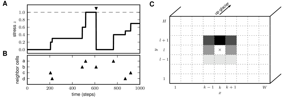
Interactions between cells. Calving of a cell at position $\{kl\}$ leads to a destabilization of its local neighborhood, mainly caused by a loss of buttress, but also due to local increases in buoyancy and changes in terminus velocity triggered by calving. In consequence, the stress level in neighboring cells $\{xy\}$ is increased (first term on rhs of (2)). For simplicity, we assume that the interaction $J_{kl}^{xy}=J(x-k,y-l)$ between cells $\{kl\}$ and $\{xy\}$ depends only on the horizontal and vertical distances $p=x-k$ and $q=y-l$, respectively. Further, we restrict the model to excitatory (positive) nearest-neighbor interactions without self-coupling, i.e.

$$J(p,q)=\begin{cases}0&\text{if $p=0$ and $q=0$}\\ 0&\text{if $|p|>1$ or $|q|>1$}\\ >0&\text{else}\,.\end{cases}$$ (3)

For the results reported in the next section, we use an asymmetric interaction kernel (see Fig. 3C)

$$J(p,q)=C\begin{cases}4&\text{if $p=0$ and $q=1$}\\ 3&\text{if $|p|=1$ and $q=1$}\\ 2&\text{if $|p|=1$ and $q=0$}\\ 1&\text{if $|p|\leq{}1$ and $q=-1$}\\ 0&\text{else}\,.\end{cases}$$ (4)

Here, $C$ is a normalization constant. The asymmetry in the vertical direction reflects that cells above the calving cell will likely experience a larger stress increment than those below due to gravity. To test whether the dynamics of the model critically depends on the specific choice of the interaction-kernel shape we also consider symmetric kernels

$$J(p,q)=C\begin{cases}1&\text{if $p=0$ and $|q|=1$}\\ 1&\text{if $|p|=1$ and $q=0$}\\ 0&\text{else}\,.\end{cases}$$ (5)

Qualitatively, the results for symmetric and asymmetric interaction kernels are the same (not shown here). Note that, with the symmetric kernel (5), our calving model is (essentially) identical to the sandpile model of ??.

To study the dependence of the calving dynamics on the coupling between cells, we consider the total calving susceptibility $w=\sum_{p}\sum_{q}J(p,q)$ as a main parameter of the model. It characterizes the overall effect of a calving cell on the ice stress in its local neighborhood. An increase in the susceptibility $w$ corresponds to a destabilization of the glacier terminus. Note that $w$ is measured in units of the critical stress $z_{\text{crit}}$; an increase in $w$ can therefore also be interpreted as a decrease in $z_{\text{crit}}$. To study the effect of ice susceptibility and/or yield stress, it is therefore sufficient to vary $w$ and keep $z_{\text{crit}}=1$ constant. Both ice susceptibility and yield stress are determined by external factors like temperature, glacier velocity, buoyancy, glacier thickness, etc.. An increase in temperature, for example, lowers the yield stress (?) and, thus, leads to an increase in the susceptibility $w$.

The calving susceptibility $w$ plays a key role for the dynamics of the calving model. To illustrate this, let’s assume that the states $z_{xy}(t)$ of the cells are uniformly distributed in the interval $[0,1]$ (across the ensemble of all cells). Calving of some cell $\{kl\}$ at time $t$ will inevitably trigger calving in any adjacent cell $\{xy\}$ with $z_{xy}(t)>1-J_{kl}^{xy}$. With the above assumption, the probability of a cell $\{xy\}$ fulfilling this condition is $J_{kl}^{xy}$. The total number of cells calving in response to a calving cell is, on average, given by the sum $\sum_{\{xy\}}J_{kl}^{xy}=w$ over all interaction strengths, i.e. by the calving susceptibility. Therefore, the calving susceptibility $w$ can be interpreted as the gain in the total number of calving cells: If $w<1$, calving activity will quickly die out. If $w>1$, the total number of calving cells tends to grow in time. For $w=1$, the system is balanced in the sense that the average total number of calving cells remains approximately constant. Strictly speaking, this holds only under the above assumption of a uniform state distribution. As illustrated in Fig. 6B,C, the cell states are indeed widely distributed over the entire stress interval $[0,1]$. Therefore, we may expect that $w=1$ marks a transition point for the dynamics of the model. In fact, as shown in Sec. 3, the variability in calving-event sizes increases substantially at $w\gtrsim{}1$ (see also ?).

Experimental protocol. Due to the above described interactions between cells, calving of individual cells may trigger calving in neighboring cells, thereby causing calving avalanches. At the beginning of each experiment, the internal ice stress of each cell was initialized by a random number drawn from a uniform distribution between $0$ and $1.1$. On average, $10\%$ of the cells were therefore above the critical stress $z_{\text{crit}}=1$ and started calving immediately. In general, this initial calving stopped after some time (see, however, Sec. 3.3). After this warm-up period, we performed a sequence of perturbation experiments: in each trial $m=1,\ldots,M$, a single cell $\{kl\}$ was randomly chosen and perturbed by a weak delta pulse $s_{\text{ext}}^{kl}(t)=\delta(t)$ of amplitude $J_{\text{ext}}=0.1$ (at the beginning of each trial, time was reset to $t=0$). The trial was finished when the calving activity in response to the perturbation had stopped. We define the number of cells calving in a single trial as the event size $\mu$. The difference $m-u$ between the id’s of two subsequent successful trials $u$ and $m>u$ ($m,u\in[1,M]$), i.e. trials with $\mu>0$, defines the inter-event interval $\tau$. Examples of calving activity in individual trials are shown in Fig. 6.

Model parameters. The model parameters are summarized in Tab. 1.

Name	Description	Value
$W$	width of glacier terminus	$\{100,200,400\}$
$H$	height of glacier terminus	$\{25,50,100\}$
$z_{\text{crit}}$	critical stress (yield stress)	$1$
$w$	calving susceptibility	$\{0.5,\ldots,1.5\}$
$J_{\text{ext}}$	perturbation amplitude	$0.1$
$M$	number of trials	$10000$

Table 1: Model parameters. Curly brackets $\{\ldots\}$ represent parameter ranges.

Simulation details. The model dynamics was evaluated numerically using the neural-network simulator NEST (?, see www.nest-initiative.org) which has been developed and optimized to simulate large systems of pulse-coupled elements. Simulations were performed in discrete time $t=0,1,2,\ldots$. Cell states were updated synchronously, i.e. calving activity at time $t$ increments the stress in neighboring cells at time $t+1$.

2.3 Data analysis

In the following, we describe the characterization of the marginal distributions and auto-correlations of event sizes and inter-event intervals. Field and model data were analyzed using identical methods. Similarly, we applied identical tools to the event sizes $\mu$ and the inter-event intervals $\tau$. Unless stated otherwise, we will therefore not distinguish between $\mu$ and $\tau$ in this subsection, and use $X$ as a placeholder.

Distributions of sizes and intervals. The overall characteristics of the distribution of data points $X_{i}$ ($i=1,\ldots,n$; $n=$ sample size) are given by its mean, standard deviation SD, minimum and maximum, and the coefficient of variation $\text{CV}=\text{SD}/\text{mean}$ (see Tab. 2). In the case of the inter-event intervals, the CV provides a measure of the regularity of the calving process: while $\text{CV}=0$ corresponds to a perfectly regular process with delta-shaped interval distribution (clock), $\text{CV}=1$ is characteristic for a process with exponential interval distribution, e.g. a Poisson point process (?). Histograms of the data on a logarithmic scale (relative frequency: number of observations within an interval $[\text{log}_{10}\left(X\right),\text{log}_{10}\left(X\right)+\text{log}_{10}\left(\Delta{}X\right))$ normalized by $n$) are used for graphical illustration of the entire distributions. As shown in Fig. 5B–G, Fig. 7A,D and Fig. 9 (symbols), the empirical distributions obtained this way are broad and resemble power-law or exponential distributions. Note, however, that such histograms, obtained by binning of finite data sets, are generally biased and therefore not appropriate for a quantitative analysis (?). Here, we applied maximum-likelihood (ML) methods (see ?) to quantify to what extent the field and model data $X$ can be explained by an exponential or a power-law distribution:

$$p_{\text{ex}}(X) =N_{\text{ex}}\begin{cases}e^{-\lambda{}X}&0\leq{}X_{\text{min}}\leq{}X\leq{}X_{\text{max}}\\ 0&\text{else}\end{cases}$$ (6)

$$p_{\text{pl}}(X) =N_{\text{pl}}\begin{cases}X^{-\gamma}&0\leq{}X_{\text{min}}\leq{}X\leq{}X_{\text{max}}\\ 0&\text{else}\end{cases}.$$ (7)

The cutoffs were set to the observed minimum and maximum, respectively: $X_{\text{min}}=\min_{i}(X_{i})$, $X_{\text{max}}=\max_{i}(X_{i})$. The prefactors $N_{\text{pl}}$ and $N_{\text{ex}}$ are normalization constants. The exponents $\lambda$ and $\gamma$ were obtained by maximizing the log-likelihoods $l_{\text{ex}/\text{pl}}=\text{E}_{i}\left[\log(p_{\text{ex}/\text{pl}}(X_{i}))\right]$ for the two model distributions. Here, $\text{E}_{i}\left[\ldots\right]=\frac{1}{n}\sum_{i=1}^{n}\ldots$ denotes the average across the ensemble of data points. The quality of the ML fits (goodness-of-fit test) was evaluated as described by ? using surrogate data and Kolmogorov-Smirnov statistics. The resulting $p$-values indicate how well the data can be explained by the model distributions $p_{\text{ex}}(X)$ or $p_{\text{pl}}(X)$. The log-likelihood ratio $R=l_{\text{pl}}-l_{\text{ex}}$, the difference between the maximum log-likelihoods, is used to judge which of the two hypotheses, the power-law or the exponential model, fits the data better. $R>0$ indicates that the power-law model $p_{\text{pl}}(X)$ is superior (and vice versa for $R<0$). The variance of $R$, estimated as $\text{E}_{i}\left[(R_{i}-R)^{2}\right]$ with $R_{i}=\log(p_{\text{pl}}(X_{i}))-\log(p_{\text{ex}}(X_{i}))$ for the best-fit distributions, was used to test whether the measured log-likelihood ratio $R$ differs significantly from zero (for details, see ?).

Auto-correlations. To investigate whether calving event sizes and intervals are informative about future events, we calculated the normalized auto-correlations (see Fig. 11)

$$a(i)=\frac{\text{E}_{j}\left[\tilde{X}(j)\tilde{X}(j+i)\right]}{\text{E}_{j}\left[\tilde{X}(j)^{2}\right]}$$ (8)

with $\tilde{X}_{j}=X_{j}-\text{E}_{j}\left[X_{j}\right]$.

Software. The data analysis was performed using Python (http://www.python.org) in combination with NumPy (http://numpy.scipy.org) and SciPy (http://scipy.org). Results were plotted using matplotlib (http://matplotlib.sourceforge.net).

3 Results

Calving at the termini of tidewater glaciers often occurs as a sequence of events, thereby showing the characteristics of avalanches: an initial detachment of small ice blocks can cascade to events of arbitrary size (see Fig. 4). In this article, we propose that the underlying dynamics can be understood as a result of the mutual interplay between calving and the destabilization of the local neighborhood of the calving region. By means of a simple calving model (see Sec. 2.2), we show that this mechanism is sufficient to understand the variability in event sizes and inter-event intervals observed in the field data (see Sec. 3.1). Fluctuations in external parameters may additionally contribute to the calving variability but are not required to explain the data. This is confirmed by our observation that changes in air temperature and tides do not affect the shape of the size and interval distributions obtained from the field data (see Sec. 3.2). The simple calving model enables us to study the effect of glacier parameters on the distributions of event sizes and intervals in a controlled manner. An increase in the calving susceptibility leads to broader event-size distributions. At a critical susceptibility, the model glacier undergoes a transition to a regime where a small perturbation leads to ongoing calving activity (see Sec. 3.3). Finally, we show that the simple calving model is consistent with the field data in the sense that the size of future calving events is not correlated with the size of past events. Predicting event sizes from past events is thus difficult, if not impossible (see Sec. 3.4).

Figure 4: Typical calving sequence observed on August 16, 2009, 21:46 GMT, at Kronebreen. The detachment of small ice blocks (B,C) triggers a large column drop with the entire height of the terminus collapsing vertically (D–G), followed by large column-rotation events with blocks of ice rotating during their fall (H–J). Time distance between consecutive images is $3\,\text{s}$. Black arrow and ellipses mark location of individual calving events.

3.1 Variability of event sizes and inter-event intervals

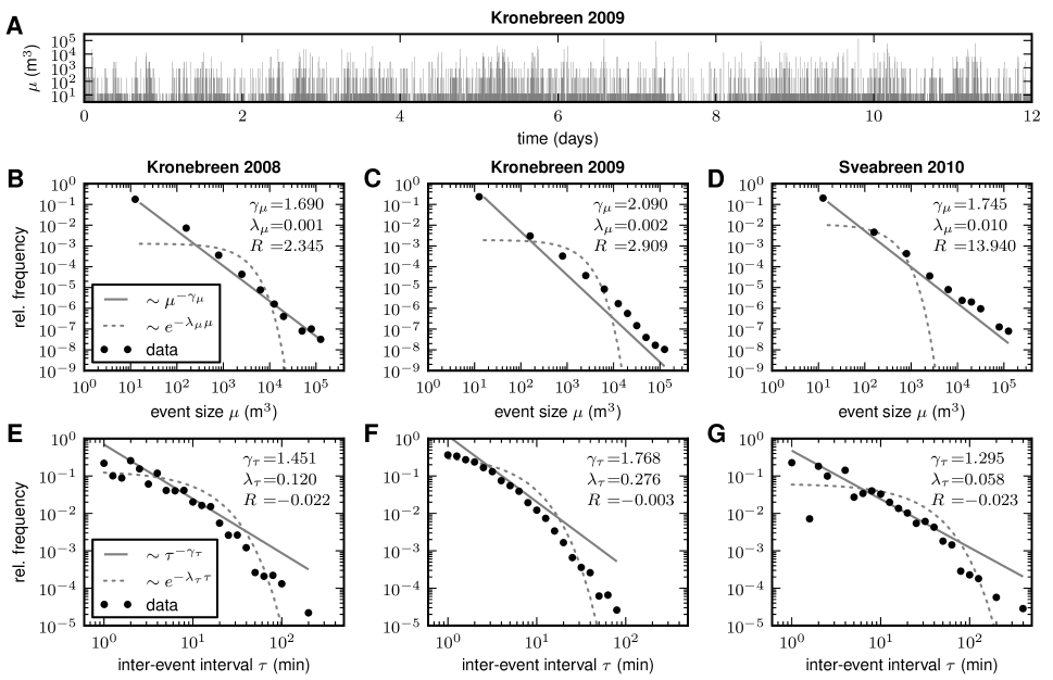
We analyzed data obtained from two glaciers on Svalbard, Kronebreen and Sveabreen, during three continuous observation periods with more than $7000$ calving events in total. The longest observation period lasted $12$ days with $5868$ events (Fig. 5A). An overview of the three data sets and the basic event-size and interval statistics is provided in Tab. 2.

The sizes $\mu$ of monitored events are highly variable. They extend over $4$ orders of magnitudes, from about $10\,\text{m}^{3}$ up to more than $10^{5}\,\text{m}^{3}$ (symbols in Fig. 5B–D). The event-size coefficient of variation (CV) varies between $6.2$ and $8.2$; the standard deviations are substantially larger than the mean values ($542$–$1512\,\text{m}^{3}$). The distributions of event sizes exhibit long tails and resemble power laws (7). Maximum-likelihood (ML) fitting yields power-law exponents $\gamma_{\mu}$ between $1.7$ and $2$ (solid gray lines in Fig. 5B–D). Note, however, that the $p$-values of the goodness-of-fit test (see Sec. 2.3) are in all cases very small, thereby indicating that the power-law model does not perfectly explain the event sizes. Still, the power-law model (7) fits the event sizes $\mu$ better than the exponential model (6) (dashed curves in Fig. 5B–D); the log-likelihood ratios $R$ are in all cases significantly greater than zero ($R=2.3$ to $14$).

The inter-event intervals $\tau$ span more than $2$ orders of magnitude ($1\,\min$ up to more than $400\,\min$; symbols in Fig. 5E–G). The standard deviations exceed the mean durations between two events ($3$–$17\,\min$) by a factor of $\text{CV}=1.5$ to $1.9$. Hence, the calving process is highly irregular; substantially more irregular than a Poisson point process with exponential interval distribution ($\text{CV}=1$; ?). The interval distributions have a longer tail than predicted by the exponential model (6) (dashed curves in Fig. 5E–G), but fall off more rapidly than the power-law model (7) (solid gray lines in Fig. 5E–G). The log-likelihood ratios $R\approx{}0$ confirm that the inter-event intervals $\tau$ are neither exponentially nor power-law distributed.

	Kronebreen		Sveabreen
	2008	2009	2010
Total number of events	1041	5868	386
Observation duration (days)	4	12	4
Start date	26 Aug.	14 Aug.	17 July
End date	1 Sept.	26 Aug.	21 July
Event sizes $\mu$
Mean ($\text{m}^{3}$)	803	542	1512
Standard deviation SD ($\text{m}^{3}$)	6599	4014	9363
Coefficient of variation CV	8.2	7.4	6.2
Minimum ($\text{m}^{3}$)	13	13	13
Maximum ($\text{m}^{3}$)	135070	135070	135070
Inter-event intervals $\tau$
Mean (min)	8	3	17
Standard deviation SD (min)	14	5	32
Coefficient of variation CV	1.7	1.5	1.9
Minimum (min)	1	1	1
Maximum (min)	201	98	446

Table 2: Overview of the three field-data sets with event-size and interval statistics.

Figure 5: Field data. A: Example time series for 12 observation days at Kronebreen (2009). Each bar represents a calving event of size $\mu$ (log scale). B–G: Distributions (log-log scale) of iceberg sizes $\mu$ (B–D) and inter-event intervals $\tau$ (E–G) for Kronebreen 2008 (B,E), 2009 (C,F) and Sveabreen 2010 (D,G). Field data (symbols), best-fit power-law (solid lines; decay exponents $\gamma_{\mu}$, $\gamma_{\tau}$) and exponential distributions (dashed curves; decay exponents $\lambda_{\mu}$, $\lambda_{\tau}$). $R$ represents corresponding log-likelihood ratio.

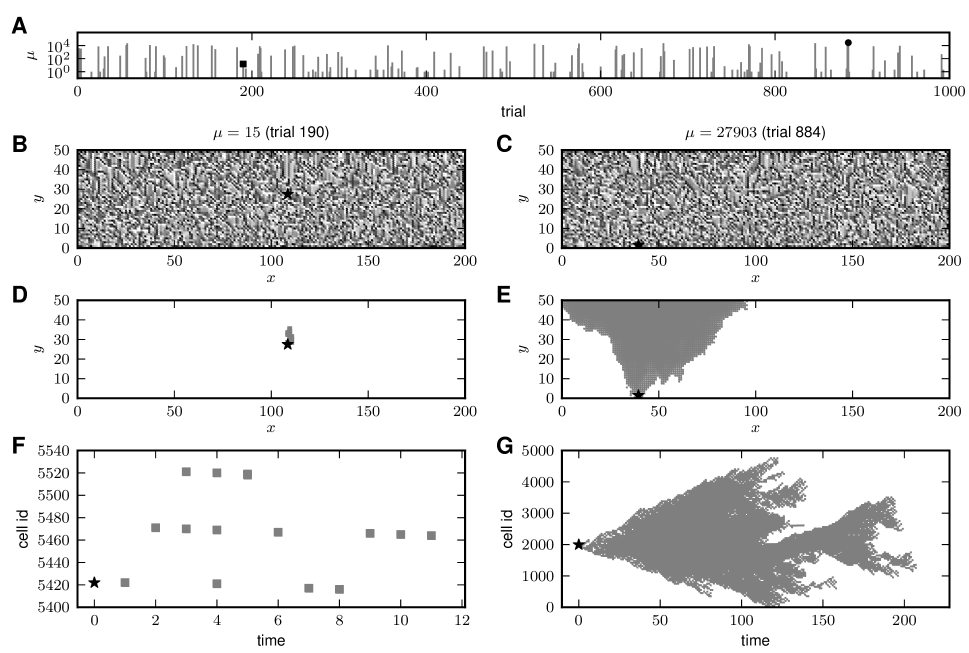
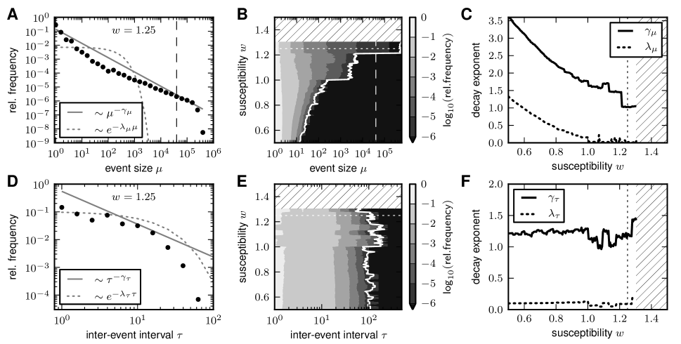
The simple calving model reproduces well the characteristics of the event-size and interval distributions obtained from the field data. An example time series generated by the calving model is depicted in Fig. 6A for a susceptibility of $w=1.3$. Small random perturbations of the model glacier lead to responses with broadly distributed magnitudes. In most cases, there is no response at all ($\mu=0$). Small events are frequently triggered (see example in Fig. 6B,D,F), whereas large events are rare (see example in Fig. 6C,E,G).

Figure 6: Size and duration variability of calving events in response to random external perturbations (model results). A: Glacier responses (event size $\mu$; log scale) to $1000$ consecutive random perturbations. Black square (trial 190) and circle (trial 884) mark events shown in B,D,F and C,E,G, respectively. B–G: Moderate-size (B,D,F; $\mu=15$) and large calving event (C,E,G: $\mu=27903$) in response to punctual random perturbations (perturbation sites indicated by black stars) in trials 190 and 884, respectively. B,C: Distribution of stress $z_{xy}$ (gray coded) across the model-glacier terminus after calving response. D,E: Spatial spread of single-trial calving activity across the model glacier terminus. Gray dots mark cells which have calved. F,G: Spatio-temporal spread of the events shown in D,E (id of cell at position $(x,y)$ $=Hx+y$; discrete time). Note different scales in F and G. Glacier width $W=200$, glacier height $H=50$, calving susceptibility $w=1.3$.

As in the field data, the distributions of event sizes $\mu$ generated by the calving model resemble power-law distributions (Fig. 7A). The width of the size distribution increases with the calving susceptibility $w$ (Fig. 7B) while the power-law exponent $\gamma_{\mu}$ decreases and approaches $1$ for $w=1.3$ (solid curve in Fig. 7C). Log-likelihood ratios $R$ are always positive and increase with $w$ (data not shown), thereby indicating that the power-law model (7) fits the data better than the exponential model (6). For $w=1.3$, the size distribution spans about $6$ orders of magnitudes ($\mu=1,\ldots,10^{6}$). Note that the maximum event size can exceed the system size $WH$ (dashed vertical lines in Fig. 7A,B) as a single cell can calve several times during one event (trial).

The inter-event intervals $\tau$ obtained from the calving model span about $2$ orders of magnitude (Fig. 7D,E). In contrast to the event-size distributions, the width of the interval distribution is independent of the calving susceptibility $w$ (Fig. 7E). ML fitting of the power-law (7) and the exponential model (6) yields exponents $\gamma_{\tau}$ and $\lambda_{\tau}$ which are comparable to those obtained for the field data (compare Fig. 7F and Fig. 5E–G). The log-likelihood ratios $R$ are always close to zero (data not shown), again consistent with the field data.

Note that the calving variability arising from the model is not a mere result of the randomness of the external perturbations (see Sec. 2.2, Experimental protocol). Restricting the repeated external perturbations to one and same cell in the center $\{W/2,H/2\}$ of the terminus results in slightly narrower but qualitatively similar event-size and interval distributions (data not shown).

Figure 7: Size (top row) and inter-event interval distributions (bottom row) generated by the calving model. A,D: Distributions (log-log scale) of iceberg sizes $\mu$ (A) and inter-event intervals $\tau$ (D) for calving susceptibility $w=1.25$. Simulation results (symbols), best-fit power-law (solid lines) and exponential distributions (dashed lines). B,E: Dependence of size and interval distributions (log-log scale) on calving susceptibility $w$. Solid white curves mark maximum sizes and inter-event intervals. C,F: Dependence of decay exponents of best-fit power-law (solid lines; $\gamma_{\mu}$, $\gamma_{\tau}$) and exponential distributions (dotted lines; $\lambda_{\mu}$, $\lambda_{\tau}$) on calving susceptibility $w$.. Glacier width $W=400$, glacier height $H=100$. Vertical dashed lines in A and B indicate system size $WH=40000$. Dotted horizontal and vertical lines in B,E and C,F, respectively, mark susceptibility $w=1.25$ used in A and D. Hatched areas in B,C,E,F correspond to regions with ongoing, self-sustained calving (see Sec. 3.3).

3.2 Impact of external parameters

As shown in the previous subsection, the calving model generates broad distributions of event sizes and inter-event intervals, even under perfectly stationary conditions. Fluctuations in external parameters are therefore not required to explain the event-size and interval variability observed in the field data. Here, we further support this finding by analyzing the relation between calving activity and fluctuations in air temperature and tides during the observation period. Both tides and temperature can, in principle, affect calving activity. High tides increase buoyant forces, thereby destabilizing the glacier terminus. An increase in temperature lowers the yield stress (?) and therefore leads to an increase in the calving susceptibility $w$. Hence, one may expect that temperature and tide-level fluctuations lead to changes in the calving-event size and interval statistics, and thereby explain the large variability reported in Sec. 3.1 (see Fig. 5).

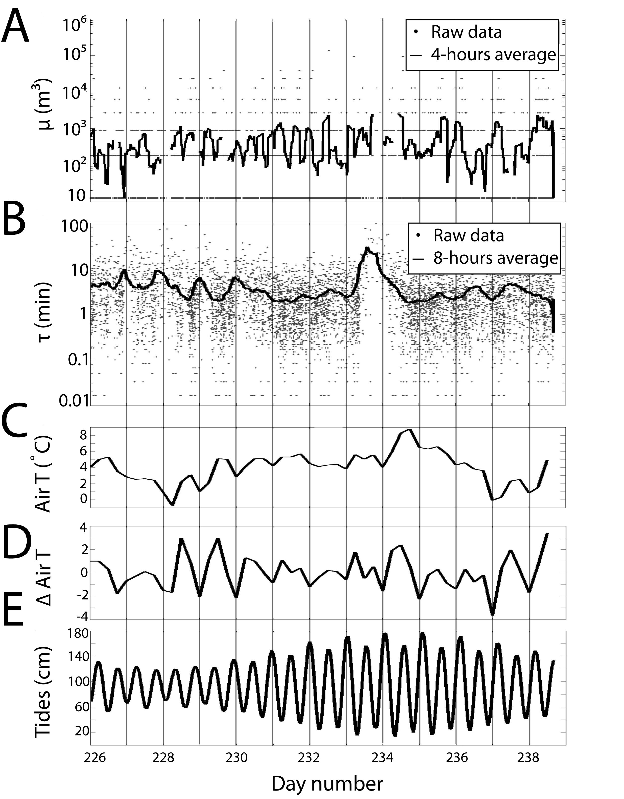
Fig. 8 depicts the simultaneous time series for event sizes (A), inter-event intervals (B), air temperature (C), change in air temperature (D), and tidal amplitude (E) during the $12$-days observation period in 2009 at Kronebreen. Within this sampling period, temperatures varied between $-0.8$ and $8.8\,^{\circ}\text{C}$, tide levels between $14$ and $178\,\text{cm}$. Significant correlations between climatic parameters and calving activity are not observed.

Figure 8: Relation between calving and external parameters (field data, Kronebreen, 2009). A: Event sizes $\mu$ (log scale). Individual events (dots) and $4$-hour average (black curve). B: Inter-event intervals $\tau$ (log scale). Individual events (dots) and $8$-hour average (black curve). C: Air temperature (Ny-Ålesund, Norwegian Meteorological Institute). D: Change in air temperature within $6$ hours. E: Tidal amplitude (Norwegian Mapping Authorities).

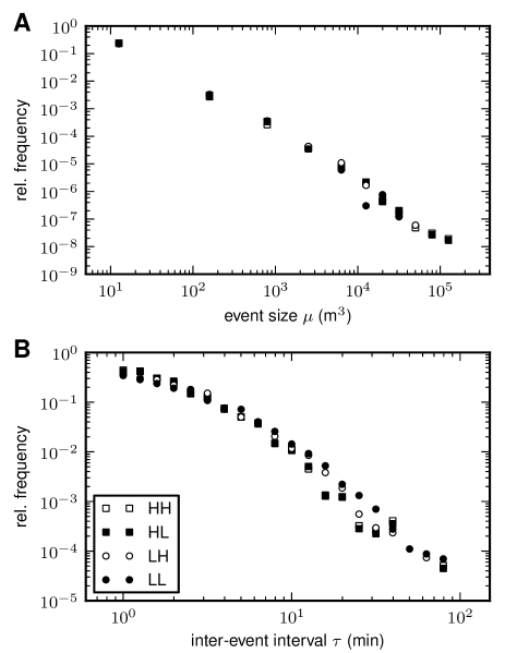
To test whether fluctuations in air temperature and tidal amplitude have an effect on the overall shape of the event-size and interval distribution, we grouped the data into high/low temperature/tide intervals. The event-size and interval histograms obtained for each group are indistinguishable (Fig. 9). Hence, the fluctuations in air temperature and tides within the observation period have no effect on the shape of the distributions. They cannot explain the observed event-size and interval variability. This does not imply that changes in temperature and tides do not affect the calving statistics in general. Long-term observations are required to investigate how larger modulations in temperature and tide levels (e.g. seasonal fluctuations) affect the shape of the event-size and interval distributions (see Sec. 4).

From the results reported here, we cannot exclude the possibility that fluctuations in other parameters, for example changes in glacier velocity or buoyancy, contribute to the size and interval variability. Note, however, that both glacier velocity and buoyancy are affected by calving itself (?). They are not purely “external” parameters. In our simple model, the positive-feedback loop between calving and these parameters is abstracted in the form of the (positive) interaction kernel (see Sec. 2.2). Hence, correlations between calving activity and fluctuations in glacier velocity or buoyancy can arise naturally from the local calving dynamics at the glacier terminus.

Figure 9: Distributions of iceberg sizes $\mu$ (A) and inter-event intervals $\tau$ (B) for four different combinations of air-temperature and tide ranges (Kronebreen, 2009; log-log scaling): high temperature – high tide (HH), high temperature – low tide (HL), low temperature – high tide (LH), low temperature – low tide (LL). Low/High air-temperature interval: $-0.8$–$4.2$/$4.2$–$8.8\,^{\circ}\text{C}$, Low/High tide-level interval: $14$–$92$/$92$–$178\,\text{cm}$.

3.3 Self-sustained calving

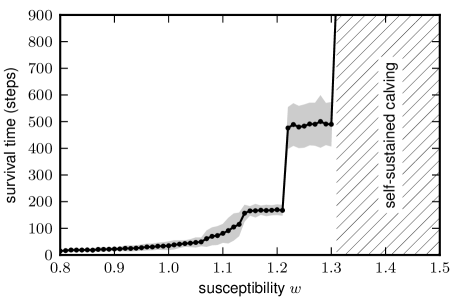
For susceptibilities $w\leq{}1.3$, small perturbations of the model glacier result in calving responses with finite life time (see e.g. Fig. 6F,G). Calving of a single cell can trigger an avalanche which sooner or later fades away and stops. For $w>1.3$, the model glacier enters a new regime where the avalanche life times seem to diverge (hatched areas in Fig. 7B,C,E,F). We illustrate this by randomly initializing the model glacier such that only a small fraction ($1\%$) of cells is superthreshold ($z>1$) at time $t=0$ and hence starts calving immediately, simulating the model glacier until this initial calving stops and measuring the corresponding survival time for a broad range of susceptibilities $w=0.8,\ldots,1.5$ (see Fig. 10). For $w>1$, the survival time quickly increases with $w$ and diverges at about $w=1.3$. Beyond this critical susceptibility, calving never stopped within the maximum simulation time (here $900$ time steps). Note that this behavior is robust and does not critically depend on the choice of other model parameters such as the terminus dimensions ($W$, $H$) and the shape of the interaction kernel (3). In all cases, we observe a critical susceptibility close to $w=1.3$ (data not shown here).

Figure 10: Survival time of calving activity after random stress initialization (with $1\%$ of the cells being superthreshold, $z_{xy}>1$, at time $t=0$) as function of calving susceptibility $w$. Mean survival time (black circles) and mean $\pm 2$ standard deviations (gray band) for $100$ random glacier initializations. Glacier width $W=400$, height $H=100$.

3.4 Predictability

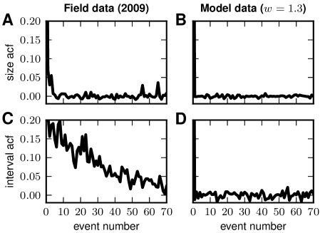
In the field data, the average correlation between the sizes $\mu_{j}$ and $\mu_{j+i}$ of subsequent events $j$ and $j+i$ hardly differs from zero for all $i>0$ (Fig. 11A). Hence, predicting future event sizes from past events appears hopeless. This behavior is reproduced by the simple calving model (Fig. 11B). The inter-event intervals $\tau$ obtained from the field data exhibit a moderate long lasting correlation which is not observed in the model data (Fig. 11C,D). The reason of this discrepancy between the model and the field data is unclear, but we suspect that it is due to non-stationarities in the field data (see Fig. 8B) which are, by construction, absent in the model.

Figure 11: Auto-correlation function (acf) for sizes (A, B) and inter-event intervals (C,D) in the field (A,C) and model data (B,D).

4 Discussion

We showed that calving-event sizes and inter-event intervals obtained from direct continuous observations at the termini of two tidewater glaciers are highly variable and broadly distributed. We demonstrated that the observed variability can be fully explained by the mutual interplay between calving and the destabilization of the local neighborhood of the calving region. A simple calving model accounting for this interplay reproduces the main characteristics of the event-size and interval statistics: i) Event-size distributions resemble power laws with long tails spanning several orders of magnitude. ii) Interval distributions are broad but fall off more rapidly than power laws. iii) Correlations between the sizes of subsequent events vanish. We conclude that the observed calving variability is a characteristic feature of calving and is not primarily the result of fluctuating external (e.g. climatic) conditions. Event sizes of all magnitudes have to be expected, even under ideal stationary conditions.

The calving model predicts that the width of the event-size distribution depends on a parameter $w$ representing the calving susceptibility of the glacier terminus: roughly, $w$ measures how prone the glacier is to calve in response to calving. It describes to what extent calving increases the internal ice stress in the neighborhood of the calving region. Alternatively, $w$ may represent the inverse of the yield stress, i.e. the critical stress at which ice breaks. The susceptibility $w$ is determined by the properties of the ice and by factors like temperature, glacier velocity, buoyancy or glacier thickness. In our model, the width of the event-size distribution increases monotonously with $w$. Therefore, the shape of the size distribution, as, for example, characterized by the power-law exponent $\gamma_{\mu}$, may be informative about the stability of the glacier terminus. In contrast to the event-size distributions, the shape of the inter-event interval distribution is insensitive to the susceptibility $w$. At a critical susceptibility $w_{\text{crit}}$, the model predicts an abrupt transition of the glacier to a new regime characterized by ongoing, self-sustained calving activity. Observations of rapid glacier retreats (???) may be explained by these supercritical dynamics (see also ?). In the model, the power-law exponent $\gamma_{\mu}$ is close to $1$ as the susceptibility approaches the critical value $w_{\text{crit}}$ (see solid curve in Fig. 7C). We found that this observation does not critically depend on the choice of the model parameters (glacier dimensions, shape of the interaction kernel, perturbation protocol). This suggests that the power-law exponent $\gamma_{\mu}$ may serve as an indicator of a glacier’s proximity to the transition point where it starts retreating rapidly. ? proposed a similar stability criterion which depends on various geometric and dynamical near-terminus parameters. In our case, the diagnostics is exclusively based on the distribution of event sizes.

The calving model in this study is inspired by previous work on the emergence of power-law distributions. Power-law shaped magnitude distributions are abundant in nature. They are found, for example, for earthquake magnitudes (??), luminosity of stars (?), avalanche sizes in sandpiles (?), landslide areas (?), subglacial water pressure pulses (?), dislocation avalanches in ice (?), and sea ice fracturing (?). ? demonstrated that power-law distributions can arise naturally in spatially extended dynamical systems which have evolved into “self-organized critical states” consisting of minimally stable clusters of all length scales. Perturbations can propagate through the system and evoke responses characterized by the absence of spatial and temporal scales (avalanches). The calving model used in the present study is qualitatively similar to the sandpile model of ?. It is therefore not surprising that it predicts power-law shaped event-size distributions. The scientific value of this part of our work exists in mapping the original model by ? to the dynamics of glacier calving and in relating the model parameters to physical measures. Moreover, the phenomenon of self-sustained ongoing activity has, to our knowledge, never been reported so far in this context.

Several aspects of this work may be subject to criticism and improvement, in particular the data acquisition and the construction of the calving model: direct visual observation by humans is so far one of the most reliable methods to monitor individual calving events in continuous time (?). However, the results are hard to reproduce exactly: due to the sporadic unpredictable nature of calving, it is difficult to capture each event. Different observers may be in different attentive states. Each new observer needs to adjust her- or himself to a common scale of perceived sizes $\psi$. To minimize the variability in perceived sizes, we arranged test observations where all observers were simultaneously confronted with size estimates (see Sec. 2.1). To confirm our findings on the relation between the shape of the event-size distribution and the state of the glacier, more data are needed from glaciers in different environments (freshwater, floating tongue, iceshelves) and different dynamical states (advancing, stable, retreating). To test our stability criterion one would need to continuously monitor the same glacier year after year for a few days. Long-term continuous observations or observations in cold months are difficult. Automatic monitoring would therefore be highly desirable. Unfortunately, all available automatic monitoring methods have limitations. Terrestrial photogrammetry, for example, is limited by the iceberg size, visibility and illumination of the glacier. Iceberg size and type also limit the use of ground-based radar. ? showed that radar could only detect events larger than $150\,\text{m}^{3}$. Remote sensing (optical and radar imagery) has the same limitations as terrestrial photogrammetry. In addition, its low temporal resolution does not allow individual calving events to be registered. Seismic monitoring (?) is a very promising technique, but can detect only the largest events (?). The range of event sizes accessible by seismic methods may however be sufficient to estimate power-law exponents. A major problem in studying the statistics of individual calving events is to define what a single event actually is. In the framework of our model, an event is defined as the total response to a single perturbation. In our numerical experiments, a new perturbation is not applied before the response to the previous perturbation has stopped. In nature, however, the glacier terminus may be constantly perturbed, e.g. by the movement of the glacier. Several events may be triggered simultaneously in neighboring regions of the terminus and, hence, overlap both spatially and temporally. The separation of individual events in the field data can therefore be difficult. In consequence, short intervals and small events may be underestimated.

The calving model used in this study is highly minimalistic. It implements the mechanism which we think is essential for an understanding of the calving variability observed in the field data (i.e. a positive-feedback loop between calving and destabilization of the glacier terminus), but neglects a variety of factors: first, the model is two-dimensional. Stress can only propagate tangentially and not in the third dimension perpendicular to the terminus. Extending the model to three dimensions is not straightforward, as it is unclear how calving at the terminus affects regions deeper within the ice body. Second, the interaction kernel is restricted to nearest-neighbor interactions. Whether and how calving affects regions more distant from the calving region is unclear. A direct measurement of the interaction kernel in the field is difficult as it would require monitoring of changes in ice stress in response to individual calving events. Conclusions on the shape of the interaction kernel could be drawn indirectly from the spatial structure of calving avalanches (e.g. obtained by terrestrial photogrammetry). For illustration, consider Fig. 6E: the triangular shape of this large event is a direct consequence of the asymmetry of the interaction kernel (4) (see Fig. 3C). For symmetric kernels (5), we observed that the spatial structure of calving events is, on average, symmetric (data not shown here). Note, however, that for the main findings of our study, the exact shape of the interaction kernel is not critical. Third, the relationships between the susceptibility $w$ (the area of the interaction kernel, see Sec. 2.2) and external parameters such as air temperature, tides, glacier velocity or buoyancy are unclear. These relationships could be established empirically from a larger data set obtained from continuous long-term observations of different glaciers during different dynamical states. For each identified set of external parameters, our model could be fitted to the distribution of monitored event sizes, thereby providing an estimate of $w$. Based on these relationships, the event-size distributions for a new “test” data set (i.e. for data not used for the fitting procedure) could be predicted by the model and compared to the field-data distributions. Fourth, stress increments in response to calving or external perturbations are instantaneous in the model. In reality, these interactions are likely to be smoother and delayed. Detailed information about this is however limited. Fifth, in the absence of calving and external perturbations, internal ice stress in a given model cell is constant. In real ice, stress in a certain volume element may slowly dissipate and decay to zero. We assume that the time constant of this decay is much larger than the time between two (external or internal) perturbations and therefore can be approximated as being infinite. Sixth, external perturbations are modeled as punctual (delta-shaped) events in time and space to characterize the system’s response in a well defined manner (i.e. to evoke responses without spatio-temporal overlap; see above). In reality, external perturbations are spatially and temporally distributed (e.g. glacier movement, glacier velocity gradients, buoyancy). Finally, the model neglects submarine calving which, in reality, amounts for about $13\%$ of the total ice loss at the terminus. One way to account for the submarine dynamics would be to assign different calving susceptibilities to the subaerial and the submarine parts. Our model describes calving at the level of individual events and focuses on a single aspect of calving: the interplay between calving and terminus destabilization. Factors like air temperature, water depth, height-above-buoyancy, surface melt, ice thickness, thickness gradient, strain rate, mass-balance rate, backward melting of the terminus, etc., are included indirectly or lumped together and treated as constant parameters. Previous macroscopic models (?????????) relate these factors to the overall calving rate. A description of size and timing of individual calving events is beyond the scope of most of these models. Our model could be connected to these models by linking the overall calving rate to the calving susceptibility or the characteristics of external perturbations. The resulting multi-scale model would have the potential to describe the statistics of event sizes and inter-event intervals under more realistic non-stationary conditions. The rationale behind the simplistic approach presented in our study is the opposite: to construct a minimal model which reproduces the main characteristics of the event-size and interval statistics. Disconnecting the glacier terminus from the external world allows us to study calving dynamics under ideal stationary conditions and to demonstrate that the observed calving variability is not primarily a result of fluctuations in external conditions, but can emerge from simple principles governing the dynamics directly at the glacier terminus.

5 Acknowledgments

We acknowledge support by the Research Council of Norway (IPY-GLACIODYN [project 176076], eVITA [eNEURO], Notur), the Helmholtz Association (HASB and portfolio theme SMHB), the Jülich Aachen Research Alliance (JARA), EU Grant 269921 (BrainScaleS) and the Svalbard Science Forum. We thank the “Young Explorers and Leaders” of the “British Schools Exploring Society Arctic Adventure” expedition in 2010 for providing the iceberg-calving data for Sveabreen. We are grateful to Abigail Morrison, Cecilie Denby-Rolstad and the two reviewers for their valuable comments on the manuscript.

Bibliography

- Amundson, J.M., and Truffer, M. 2010. A unifying framework for iceberg-calving models. J. Glac., 56, 199, 822–830.
- Bak, P. 1996. How Nature Works: The science of self-organized criticality. Springer, Copernicus, New York, Springer.
- Bak, P., Christensen, K., Danon, L., and Scanlon, T. 2002. Unified scaling law for earthquakes. Phys. Rev. Lett., 88.
- Bak, P., Tang, C., and Wiesenfeld, K. 1987. Self-organized criticality - An explanation of 1/f noise. Phys. Rev. Lett., 59, 381–384.
- Bak, P., Tang, C., and Wiesenfeld, K. 1988. Self-organized criticality. Phys. Rev. A, 38, 364–374.
- Bahr, D. B. 1995. Simulating iceberg calving with a percolation model. J. Geophys. Res., 100, 6225–6232.
- Bassis, J.N. 2010. The statistical physics of iceberg calving and the emergence of universal calving laws. J. Glac., 57, 57, 3–16.
- Benn, D.I., Warren, C.R., and Mottram, R.H. 2007 (a). Calving processes and the dynamics of calving glaciers. Earth-Sci. Rev., 82, 143–179.
- Benn, D.I., Hulton, N.R.J., and Mottram, R.H. 2007 (b). ‘Calving laws’, ‘sliding laws’ and the stability of tidewater glaciers. A. Glac., 46, 123–130.
- Briner J.P., Bini A.C., Anderson R.S. 2009. Rapid early Holocene retreat of a Laurentide outlet glacier through an Arctic fjord. Nat. Geosci., 2 (7), 496–499.
- Brown, C.S., Meier, M.F., Post, A. 1982. Calving speed of Alaska tidewater glaciers, with application to Columbia Glacier. U.S. Geol. Surv. Prof. Pap., 1258-C.
- Budd, W.F., Jacka, T.H., and Morgan V.I. 1980. Antarctic iceberg melt rates derived from size distributions and movement rates. Ann. Glaciol., 1, 103–112.
- Chapuis, A., Rolstad, C., and Norland, R. 2010. Interpretation of amplitude data from a ground-based radar in combination with terrestrial photogrammetry and visual observations for calving monitoring of Kronebreen, Svalbard. Ann. Glaciol., 51, 34–40.
- Clar, S., Drossel, B., Schenk, K., and Schwab, F. 1999. Self-organized criticality in forest-fire models. Physica A, 266, 153–159.
- Clauset, A., Shalizi, C.R., and Newman, M.E.J. 2009. Power-law distributions in empirical data. Siam Rev., 51, 661–703.
- Cox, D. R. 1962. Renewal Theory. Methuen, London.
- de Boer, J., Jackson, A.D., and Wettig, T. 1995. Criticality in simple models of evolution. Phys. Rev. E, 51, 1059–1074.
- Dowdeswell, J.A., and Forsberg, C.F. 1992. The size and frequency of icebergs and bergy bits derived from tidewater glaciers in Kongsfjorden, Northwest Spitsbergen. Polar Res., 11, 81–91.
- Gewaltig, M.-O., and Diesmann, M. 2007, NEST (Neural Simulation Tool). Scholarpedia, 2(4), 1430.
- Guzzetti, F., Malamud, B.D., Turcotte, D.L., and Reichenbach, P. 2002. Power-law correlations of landslide areas in central Italy. Earth Planet. Sc. Lett., 195, 169–183.
- Hainzl, S. 2003. Self-organization of earthquake swarms. J. Geod., 35, 157–172.
- Hanson, B. and Hooke LeB., R. 2000. Buckling rate and overhand development at a calving face. J. Glac., 49, 167, 577–586.
- Herz, A.V.M., Hopfield, J.J. 1995. Earthquake cycles and neural reverberations: Collective oscillations in systems with pulse-coupled threshold elements, PRL 75(6), 1222–1225.
- Hughes, T. 1986. The Jakobshavns effect. Geophys. Res. Lett., 13, 46–48.
- Kavanaugh, J.L. 2009. Exploring glacier dynamics with subglacial water pressure pulses: Evidence for self-organized criticality? J. Geophys. Res-Earth, 114.
- Köhler, A., Chapuis, A., Nuth, C., Kohler, J., and Weidle, C. 2012. Autonomous detection of calving-related seismicity at Kronebreen, Svalbard. The Cryosphere, 6, 393–406.
- Lapicque L. 1907. Recherches quantitatives sur l’excitation electrique des nerfs traitee comme une polarization. J. Physiol. Pathol. Gen., 9, 620–635.
- Motyka, R.J., Hunter, L., Echelmeyer, K.A., Connor, C. 2003. Submarine melting at the terminus of a temperate tidewater glacier, LeConte Glacier, Alaska, U.S.A.. A. Glac., 36, 57–65.
- Motyka, R.J., Truffer, M., Fahnestock, M., Mortensen, J., Rysgaard, S., Howat, I. 2011. Submarine melting of the 1985 Jakobshavn Isbr floating tongue and the triggering of the current retreat. J. Geophys. Res-Earth, 116.
- Neshyba, S. 1980. On the size distribution of Antarctic icebergs. Cold Reg. Sci. Techo Rep., 1, 241-248.
- Nick, F.M., Vieli, A., Howat, I., and Joughin, I. 2009. Large-scale changes in Greenland outlet glacier dynamics triggered at the terminus. Nat. Geosci., 2, 110–114.
- Nick, F.M., van der Veen, C.J., Vieli, A., Benn, D.I.. 2010. A physically-based calving model applied to marine outlet glaciers and implications for the glacier dynamics. J. Glac., 56, 199, 781–794.
- Oerlemans, J., Jania, J., Kolondra, L. 2011. Application of a minimal glacier model to Hansbreen, Svalbard. The Cryosphere, 5, 1–11.
- O’Neel, S., Echelmeyer, K.A., and Motyka, R. 2003. Short-term variations in calving of a tidewater glacier: LeConte Glacier, Alaska, USA. J. Glaciol., 49, 587–598.
- O’Neel, S., Marshall, H.P., McNamara, D.E., and Pfeffer, W.T. 2007. Seismic detection and analysis of icequakes at Columbia Glacier, Alaska. J. Geophys. Res., 112.
- O’Neel, S., Larcen, C.F., Rupert, N., Hansen, R. 2010. Iceberg calving as a primary source of regional-scale glacier-generated seismicity in the St. Elias Mountains, Alaska. J. Geophys. Res-Earth., 115.
- Orheim, O. 1985. Iceberg discharge and the mass balance of Antarctica. in Glaciers, Ice Sheets, and Sea Level: Effect of a CO2-induced climatic change, Report of a workshop held in Seattle Washington September 13-15, 210–215, National Academy Press, Washington, D.C.
- Otero, J., Navarro, F.J., Martin, C., Cuadrado, M.L., Corcuera, M.I. 2010. A three-dimensional calving model: Numerical experiments on Johnsons Glacier, Livingston Island, Antarctica. J. Glac., 56, 196, 200–214 .
- Pfeffer, W.T. 2007. A simple mechanism for irreversible tidewater glacier retreat. J. Geophys. Res-Earth., 112 (F3).
- Qamar, A. 1988. Calving icebergs: A source of low-frequency seismic signals from Columbia Glacier, Alaska. J. Geophys. Res-Solid, 93, 6615–6623.
- Rampal, P., Weiss, J., Marsan, D., Lindsay, R., and Stern, H. 2008. Scaling properties of sea ice deformation from buoy dispersion analysis. J. Geophys. Res-Oceans, 113.
- Reeh, N. 1968. On the calving of ice from floating glaciers and ice shelves. J. Glac., 7, 50, 215–232.
- Richeton, T., Weiss, J., and Louchet, F. 2005. Dislocation avalanches: Role of temperature, grain size and strain hardening. Acta Mater., 53, 4463–4471.
- Ritchie, J.B., Lingle, C.S., Motyka, R.J., Truffer, M. 2008: Seasonal fluctuations in the advance of a tidewater glacier and potential causes: Hubbard Glacier, Alaska, USA. J. Glaciol., 54 (186), 401–411.
- Rolstad, C., and Norland, R. 2009. Ground based interferometric radar for velocity measurements of the calving front of Kronebreen, Svalbard. Ann. Glaciol., 50, 47–54.
- Shew, W.L. and Plenz D. 2013. The functional benefits of criticality in the cortex. Neuroscientist, 19 (1), 88–100.
- Stevens, S.S. 1957. On the psychological law. Psychol. Rev., 64, 153–181.
- Tuckwell H.C. 1988. Introduction to Theoretical Neurobiology, Volume 1. Cambridge. Cambridge University Press.
- Van Der Veen, C.J. 1996. Tidewater calving. J. Glac., 141, 375–385.
- Van Der Veen, C.J. 1997. Calving glaciers: Report of a workshop. BPRC Report No.15 Byrd Polar Research Center, The Ohio State University, Columbus, Ohio, 194 pp.
- Vieli, A.,Funk, M., Blatter, H. 2001. Flow dynamics of tidewater glaciers: A numerical modelling approach. J. Glac., 47, 159, 595–606.
- Vieli, A., Jania, J., Kolondra, L. 2002. The retreat of a tidewater glacier: Observations and model calculations on Hansbreen, Spitsbergen. J. Glac., 48, 163, 592–600.
- Wadhams, P. 1988, Winter observations of iceberg frequencies and sizes in the South Atlantic Ocean. J. Geophys. Res., 93, 3583–3590.
- Warren, C.R., Glasser, N.F., Harrison, S., Winchester, V., Kerr, A.R., Rivera, A. 1995. Characteristics of tide-water calving at Glaciar San-Rafael, Chile. J. Glaciol., 41, 273–289.
- Washburn, H.B., Jr. 1936. The Harvard-Dartmouth Alaskan expeditions 1933-1934. Geogr. J., 87, 481–495.