Fast-ignition design transport studies: realistic electron source, integrated PIC-hydrodynamics, imposed magnetic fields

Abstract

Transport modeling of idealized, cone-guided fast ignition targets indicates the severe challenge posed by fast-electron source divergence. The hybrid particle-in-cell [PIC] code Zuma is run in tandem with the radiation-hydrodynamics code Hydra to model fast-electron propagation, fuel heating, and thermonuclear burn. The fast electron source is based on a 3D explicit-PIC laser-plasma simulation with the PSC code. This shows a quasi two-temperature energy spectrum, and a divergent angle spectrum (average velocity-space polar angle of $52^{\circ}$). Transport simulations with the PIC-based divergence do not ignite for $>$ 1 MJ of fast-electron energy, for a modest (70 $\mu\mathrm{m}$) standoff distance from fast-electron injection to the dense fuel. However, artificially collimating the source gives an ignition energy of 132 kJ. To mitigate the divergence, we consider imposed axial magnetic fields. Uniform fields $\sim$50 MG are sufficient to recover the artificially collimated ignition energy. Experiments at the Omega laser facility have generated fields of this magnitude by imploding a capsule in seed fields of 50-100 kG. Such imploded fields are however more compressed in the transport region than in the laser absorption region. When fast electrons encounter increasing field strength, magnetic mirroring can reflect a substantial fraction of them and reduce coupling to the fuel. A hollow magnetic pipe, which peaks at a finite radius, is presented as one field configuration which circumvents mirroring.

I Introduction

The fast ignition approach to inertial fusion exploits a short-pulse, ultra-intense laser to heat an isochoric hot spot to ignition conditions (Tabak et al., 1994). Unlike the central hot-spot approach, fast ignition separates dense fuel assembly from hot-spot formation (Basov, Gus’kov, and Feokistov, 1992). This opens the prospect of high energy gain with less laser energy, and may be an attractive avenue for inertial fusion energy. The first integrated but sub-ignition scale experiments were performed at Osaka in 2001-2002, and explored the cone-in-shell geometry (Kodama et al., 2001, 2002). Subsequent similar experiments were done at Vulcan (Key et al., 2008), Omega EP (Theobald et al., 2011), and Osaka in 2009 and 2010 (Shiraga et al., 2011; Fujioka et al., 2011). The 2002 Osaka experiments were interpreted to show high coupling of short-pulse laser energy to the fuel, of order 20%. All the later experiments show lower coupling, the best being 10-20% coupling in the 2010 Osaka experiments (Shiraga et al., 2011; Fujioka et al., 2011). This work suggests the reduced coupling seen in 2009 at Osaka was due to higher pre-pulse in the short-pulse laser. Pre-pulse energy creates an underdense pre-plasma in which the laser converts to over-energetic electrons, and this source is farther away from the fuel. The negative impact of pre-plasma on fast-electron generation inside a cone has been reported, e.g., in Refs. Baton et al., 2008; MacPhee et al., 2010; Ma et al., 2012. Coupling efficiences at small scale do not directly apply at ignition scale.

This paper presents integrated fast-ignition modeling studies at ignition scale, which is well beyond parameters currently accessible by experiment. We utilize a new, hybrid PIC code Zuma (Larson, Tabak, and Ma, 2010) to model fast electron transport through a collisional plasma, with self-consistent return current and electric and magnetic field generation. To alleviate the need to resolve light waves or background Langmuir waves, Zuma does not include the displacement current in Ampère’s law, and employs an Ohm’s law (obtained from the inertialess limit of the background electron momentum equation) to find the electric field. We recently coupled Zuma to the radiation-hydrodynamics code Hydra (Marinak et al., 2001), which has been widely used to model inertial fusion and other high-energy-density systems.

We do not model the short-pulse laser, but instead inject electrons with a specified distribution into Zuma. The source electron spectrum is a key element of this approach. We obtain the spectrum by using the particle-in-cell code PSC (Bonitz et al., 2006; Kemp, Cohen, and Divol, 2010) to perform a 3D full-PIC simulation of the laser-plasma interaction (LPI). This gives a quasi two-temperature energy spectrum, with a (cold, hot) temperature of (19, 130)% of the so-called ponderomotive temperature as defined below (Wilks et al., 1992) at the nominal laser intensity. It is generally seen in PIC simulations that LPI occurring at lower density produces more energetic electrons. The experimental understanding of fast electron energy spectra is not entirely clear. Ma et al. recently reported experimental evidence indicating a two-temperature energy spectrum (Ma et al., 2012), albeit at lower energies and shorter pulses than considered here for ignition.

The PIC-based angle spectrum is very divergent, with an average polar angle in velocity space of 52^∘ or an integrated solid angle of 4.85 sterad. A large divergence has been reported in other PIC simulations, such as Refs. Ren et al., 2006; Adam, Héron, and Laval, 2006. Experimental evidence for a significant divergence comes from modeling by Honrubia et al. (Honrubia et al., 2006) of $K_{\alpha}$ data obtained by Stephens et al. (Stephens et al., 2004). More recent work by Westover et al. (Westover et al., 2011) also indicates a substantial source divergence.

Our Zuma-Hydra modeling with a realistic fast electron source (both energy and angle spectra) and an idealized fuel mass located 70 $\mu$m from the electron source indicates poor coupling to the fuel hot spot, with $>1$ MJ of fast electrons inadequate to ignite. Artificially collimating the electron source dramatically improves the picture, with an ignition energy of 132 kJ. This is much higher than the ideal estimate of 8.7 kJ absorbed in the ignition hot spot (detailed below), due largely to the energy spectrum being too hot for the electrons to stop fully in the hot spot. In Ref. Strozzi et al., 2011, we report in more detail the effects of the energy spectrum, as well as E and B fields, on the ignition requirements for an artificially-collimated fast electron source. We merely note here that, for our particular plasma condition profiles, using the complete Ohm’s law Eq. (14) reduces the fast-electron coupling to the fuel compared to the case of no E or B fields, while using the resistive Ohm’s law $\vec{E}=\eta\vec{J}_{b}$ increases the coupling over the no-field case. This is likely due to $\nabla n_{e}\times\nabla T_{e}$ magnetic fields that develop at the outer radius of the dense fuel and push the fast electrons to larger radius, as observed earlier in Ref. Nicolaï et al., 2011.

The focus of this paper is on mitigating the beam divergence by imposed magnetic fields. In particular, we do not pursue here other attractive options, such as field generation by resistivity gradients (Robinson and Sherlock, 2007). Cylindrical (Knauer et al., 2010) and spherical (Chang et al., 2011; Hohenberger et al., 2011) implosions at the Omega laser have compressed seed magnetic fields $\sim$10 kG to strengths of 20-40 MG. We show that a uniform, initial axial field of 50 MG almost recovers the ignition energy of the artificially collimated beam. We stress that such magnetic fields do not collimate the electrons (that is, reduce the velocity-space divergence), but rather confine them in space: once they emerge from the confining field, they still have their initial divergence. A magnetic field that increases in the axial direction leads however to substantial reflection due to magnetic mirroring. We explore a hollow magnetic pipe, that peaks at a finite radius, as one method to circumvent mirroring. Pipes with a peak field of 50 MG and radial FWHM of (20, 30) $\mu$m ignite for (211, 158) kJ of fast electrons, compared with 132 kJ for an artificially-collimated source with no imposed field.

The paper is organized as follows. Sec. II describes the fast electron source derived from a full PIC simulation of the LPI. In Sec. III we detail the Zuma model, and how it is coupled to Hydra. Sec. IV presents Zuma-Hydra results with realistic fast electron divergence and an artificially collimated source. We study ways to mitigate the source divergence with several imposed magnetic fields (uniform, increasing, and a hollow pipe) in Sec. V. In Sec. VI we make some concluding remarks.

II Electron source from full-PIC laser-plasma modeling

The distribution of fast electrons produced by the short-pulse LPI is a crucial element of fast ignition. The computational scale of integrated LPI-transport-hydro simulations is currently prohibitive. We excite a fast electron source derived from full-PIC LPI simulations in our transport modeling. This neglects feedback of the transport on the LPI, e.g. the exact details of the return current, and also loses some detail in the fast-electron source. It does call out the major design challenges, and allows for the development of ideas to mitigate them.

Our LPI simulations are performed with the relativistic PIC code PSC (Bonitz et al., 2006). This code has recently been extended to include a hybrid model, valid for collisional plasmas (Cohen, Kemp, and Divol, 2010). The results presented here do not use the hybrid model, and are all explicit, full-PIC calculations, with the complete Maxwell equations and no collision operator. We note that more recent PSC simulations of several ps duration show the convergence of profiles with and without an initial pre-plasma, and the development of a third, super-hot component (temperature several times the ponderomotive value given below) besides the two components present in the results discussed here. Our source will be updated with these new results in the near future.

The specific PSC run used for the fast electron source was as follows. The geometry was 3D Cartesian, and the electron density at time 360 fs over a 2D plane is shown in Fig. 1. The domain extended from $-$30 to $+$30 $\mu\mathrm{m}$ in the two transverse ($x$ and $y$) directions and from 0 to 40 $\mu\mathrm{m}$ in $z$ (nominal direction of laser propagation). The particle and field boundary conditions (BCs) were periodic in $x$ and $y$. In $z$, the particle BCs were thermalizing re-emission, while the field BCs were radiative (outgoing-wave). The initial plasma profile was $n_{e}/n_{cr}=100$ for $z>z_{0}$ and $\exp[(z-z_{0})/3.5\,\mu\mathrm{m}]$ for $z<z_{0}$ with $z_{0}=$20 $\mu\mathrm{m}$ and $n_{cr}=1.115\cdot 10^{21}/\lambda_{0}^{2}[\mu\mathrm{m]}$ cm^-3, the non-relativistic laser critical density. This profile was chosen to replicate the pre-plasma produced by a small pre-pulse ($\sim$1-10 mJ) in the short-pulse laser (e.g. growing from ASE). Both electrons and deuterium ions ($Z/A=1/2$) were mobile. The uniform cell size was $\Delta x=\Delta y=\lambda_{0}/16$ and $\Delta z=\lambda_{0}/16.375$. The time step was $c\,\Delta t=0.421\Delta x$. There were (twelve, four) numerical macro-particles per cell for (electrons, ions). The run required about 160k cpu-hours to complete.

The laser had a vacuum wavelength of $\lambda_{0}=$1 $\mu\mathrm{m}$ and a vacuum focal spot at $z=$10 $\mu\mathrm{m}$ with radial intensity profile $I(r)=I_{0L}\exp\left[-(r/18.3\,\mu\mathrm{m})^{8}\right]$. For a given laser power and maximum (hard-edge) spot radius, a flat as opposed to peaked (e.g., Gaussian) profile reduces the average intensity and gives a cooler spectrum. We chose $I_{0L}=1.37\cdot 10^{20}$ W/cm², corresponding to a normalized vector potential $a_{0}=10$. The ponderomotive temperature, as defined in Ref. Wilks et al., 1992, for the peak laser intensity is $T_{p}/m_{e}c^{2}=\left[1+a_{0}^{2}\right]^{1/2}-1=9.05$ , or $T_{p}=4.62$ MeV. We simply use $T_{p}$ to denote an energy scale, without any implication about what the fast electron distribution is (which is discussed below). The laser pulse was ramped up to peak intensity over 30 fs.

We took all electrons at the time 360 fs, in a cylindrical “extraction box” from $z=20-25$ $\mu\mathrm{m}$ and radius 30 $\mu\mathrm{m}$. This box is deep enough into the overdense region that the laser did not propagate there. We also selected only electrons with $0.55<E\,[\mathrm{MeV]}<29.5$ (or $0.12<E/T_{p}<6.37$) and $v_{z}>0$, where $E=m_{e}c^{2}(\gamma-1)$. This is done to eliminate the return current and background heating. Some of this heating is unphysical grid heating, and some is a legitimate kinetic energy transfer between the fast electrons and the background plasma at the 100$n_{cr}$ density used in the PIC simulation for numerical reasons. This heating is expected to play a negligible role at the densities assumed in our hybrid simulations (Kemp et al., 2006).

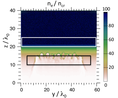
Figure 1: (Color online) Electron density at time 360 fs in the PSC run used to characterize the fast electron source. The white box indicates the extraction box, and the black box indicates the source box in the hybrid-implicit LSP run. The laser was incident from $z=0$ with a vacuum focus at $z=10$ $\mu\mathrm{m}$.

For our transport studies, we do not inject a fast electron source in an analogous extraction box. In particular, such a source would need a radially outward drift that varies with radius. Instead, we excite fast electrons in a “source box” analogous to the laser absorption region, such that after propagating a small distance into an equivalent extraction box, the transport-code electron distribution matches that of the PIC electrons. This method automatically handles a host of issues regarding propagation from the source to extraction regions (e.g., finite “view factors” that vary with angle and radius), and provides the overall laser to electron conversion efficiency. The source electron intensity is $\alpha_{CE}I(r)$ where $I(r)$ is the vacuum laser intensity given above, and $\alpha_{CE}=0.52$ is an overall laser-to-electron power conversion efficiency. $\alpha_{CE}$ was chosen so the total fast electron kinetic energy in the PSC and transport-code extraction boxes match. The source intensity is varied in space and time only by varying the rate of excitation, not the velocity-space distribution.

To arrive at the transport-code distribution excited in the source box, we performed a hybrid implicit-PIC simulation with the LSP plasma simulation code (Welch et al., 2006), with kinetic fast electrons and fluid background species (this is the only time LSP is used in this paper). The LSP source box was located from $z=$ 10 to 15 $\mu\mathrm{m}$, and the plasma was uniform 10 g/cm³ carbon at 100 eV. We used this much denser background than the PSC simulation because the fluid model is only valid at high collisionality, and our transport studies are performed in compressed matter. The difference between free-particle propagation and the full LSP results are small, indicating that forces are not important as electrons transit from source to extraction boxes.

The following LSP source gave electrons in the extraction box that agreed adequately with the PSC extraction box electrons. The source velocity-space distribution is azimuthally symmetric and given by $d^{2}N/dEd\theta=N_{0}f_{E}(E)f_{\theta}(\theta)$, so that $(f_{E},f_{\theta})$ are proportional to the 1D distributions $(dN/dE,dN/d\theta)$. $N_{0}$ is an overall normalization factor. $\tan\theta=\left[v_{z}/\left(v_{x}^{2}+v_{y}^{2}\right){}^{1/2}\right]$ defines the polar angle in velocity space. For PSC runs at ignition powers and wide focal spots, we generally find the angle spectrum does not vary much with energy (see Fig. 3). This justifies our 1D factorization; the method can be easily extended to several energy bins each with different $f_{\theta}$.

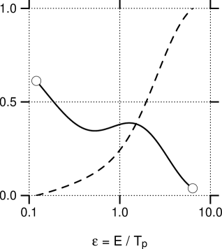
Figure 2: Source energy spectrum $E\,f_{E}$ (solid) and its running integral (dash) for the analytic form in Eq. (1). The circles indicate the limits of the domain taken in the extraction box, and injected into our Zuma-Hydra simulations.

II.1 Fast electron energy spectrum

For $f_{E}$ we use the 1D energy spectrum $dN/dE$ found in the PSC extraction box. This is well-fit by a quasi two-temperature form:

$$f_{E}(\epsilon)=\frac{1}{\epsilon}\exp\left[-\epsilon/\tau_{1}\right]+0.82\exp\left[-\epsilon/\tau_{2}\right].$$ (1)

$\epsilon\equiv E/T_{p}$ is the ponderomotively scaled energy, and we assume as we vary the laser intensity and wavelength that $dN/dE$ scales in this manner. Figure 2 plots this analytic form, as well as its running integral. The temperature-like parameters have the values $\tau_{1}=0.19$ and $\tau_{2}=1.3$. These correspond to a relatively “cold” component produced by LPI near or above $n_{cr}$, and a slightly hotter than $T_{p}$ component arising from underdense LPI. The $1/\epsilon$ factor on the cold part improves the fit at low energy, although this may change as better ways to eliminate return current and background heating are developed. We only inject over the domain $0.12<\epsilon<6.37$ , which is the domain taken from the PSC extraction box. The average injected electron energy is $\left\langle\epsilon\right\rangle=1.02$, while only 24% of the injected energy is carried by electrons with $\epsilon<1$. This is unfortunate for ignition with the laser intensities we contemplate, as discussed in Sec. IV.

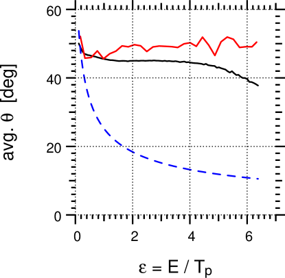
Figure 3: (Color online) Average velocity-space polar angle vs. electron kinetic energy in the extraction box for the PSC full-PIC (solid black) and LSP implicit-PIC (solid red) runs. The classical ejection angle $\theta_{c}$ from Eq. (2) is plotted in dashed blue.

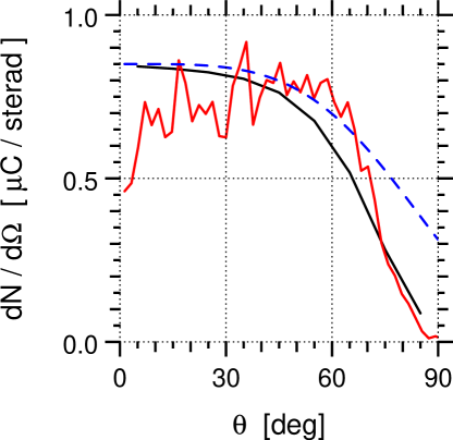
Figure 4: (Color online) Solid angle spectra in extraction box for PSC run as described in text (black), LSP run extraction box (red), and source $f_{\Omega}$ from Eq. (3) with an arbitrary scale factor (blue dashed). The source spectrum is broader than those in the extraction boxes due to limited view factor at large angles. Note that the first two curves are given in physical units.

II.2 Fast electron angle spectrum

The average angle $\theta$ in the extraction box as a function of electron energy is displayed in Fig. 3. The PSC full-PIC $\theta$ becomes slightly more collimated at higher energies, while the LSP implicit-PIC $\theta$ is essentially independent of energy. The agreement is excellent for $E<T_{p}$, but the LSP $\theta$ is slightly larger at large energies. We consider the energy dependence of $\theta$ to be weak enough to ignore and use a factorized source. Both PIC simulations have much larger $\theta$, and much less decrease with energy, than the classical ejection angle $\theta_{c}$ given by (Quesnel and Mora, 1998)

$$\tan\theta_{c}=\left[\frac{2}{\gamma-1}\right]^{1/2}.$$ (2)

This result obtains for a single electron in a focused laser beam in vacuum, not including plasma effects.

The source angle spectrum we use is

$$f_{\theta}(\theta)=2\pi\sin(\theta)f_{\Omega}\qquad f_{\Omega}=\exp\left[-\left(\theta/\Delta\theta\right)^{4}\right].$$ (3)

$\Omega$ represents solid angle, related to $\theta$ by $d\Omega=2\pi\sin(\theta)d\theta$. The value of the parameter $\Delta\theta$ that gives good agreement with the angle spectrum in the extraction box is $\Delta\theta=90^{\circ}$. Figure 4 displays the source $f_{\Omega}$ as well as the angle spectra in the PSC and LSP extraction boxes. The resulting extraction box angle spectrum is somewhat narrower than this source, due to limited view factor at large $\theta$. In addition, the LSP extraction spectrum is depleted at small angle compared to the PSC spectrum, and may slightly overstate the divergence (although there are few particles at small $\theta$ due to the $\sin\theta$ Jacobian). We stress that $\Delta\theta$ is a parameter in a function, and not an observable quantity. The average $\theta$, which has physical meaning, is

$$\left\langle\theta\right\rangle\equiv\frac{\intop_{0}^{\pi/2}d\theta\,f_{\theta}\theta}{\intop_{0}^{\pi/2}d\theta\,f_{\theta}}\approx\frac{\Gamma[3/4]}{\pi^{1/2}}\Delta\theta=0.691\Delta\theta,\,\,\,\,\,\,\,\Delta\theta<1.$$ (4)

$\Gamma$ is the mathematical gamma function. $\left\langle\theta\right\rangle$ and the rms $\theta$ are shown vs. $\Delta\theta$ in Fig. 5. Note that for large $\Delta\theta$, $\left\langle\theta\right\rangle$ falls below the approximate linear result given above. For $\Delta\theta=90^{\circ}$ we find $\left\langle\theta\right\rangle=52^{\circ}$ and rms $\theta=56^{\circ}$. The integrated solid angle $\Omega_{I}$ is $\int_{0}^{2\pi}d\Omega\,f_{\Omega}=4.85$ sterad (for an isotropic distribution, $f_{\Omega}=1$ and $\Omega_{I}=2\pi$). This is a substantial divergence; the rest of this paper is focused on its consequences for fast ignition requirements, and mitigation ideas based on imposed magnetic fields.

We briefly note that our source is symmetric in azimuthal angle. However, it quickly develops a radially outward drift as it propagates. That is, the average angle, $\chi$, between an electron’s position and velocity vectors decreases. For free motion, in the far-field limit they become parallel: $\vec{r}\approx\vec{v}t$. In the extraction box the LSP and PSC electrons have similar $\chi$ distributions vs. radius. Debayle (Debayle et al., 2010) has recently discussed the role of an intrinsic radial drift produced by a Gaussian laser; we find such a drift naturally develops due to propagation from a symmetric source.

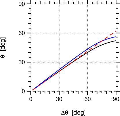
Figure 5: Average (solid black) and rms (solid blue, slightly higher) polar angle for the angle spectrum in Eq. (3), vs. the parameter $\Delta\theta$. The red dashed line is the approximate form $\left\langle\theta\right\rangle=0.691\Delta\theta$ from Eq. (4).

III Zuma-Hydra integrated modeling

Our transport modeling is done with the hybrid-PIC code Zuma (Larson, Tabak, and Ma, 2010) coupled to the radiation-hydrodynamics code Hydra (Marinak et al., 2001). We describe here the Zuma model in some detail, and how it is coupled to Hydra. We briefly discuss how we run Hydra, and refer the reader to the extensive literature on this well-established code.

III.1 Zuma hybrid-PIC code

Zuma is a parallel, hybrid-PIC code that currently supports 3D Cartesian and 2D cylindrical RZ geometry. It employs an explicit time-stepping approach, treats the fast electrons by a standard, relativistic PIC method, and models the background plasma as a collisional fluid. The electric field is found from Ohm’s law (i.e., the momentum equation for the background electrons in the limit $m_{e}d\vec{v}_{eb}/dt\rightarrow 0$), and the background return current is found from Ampère’s law without displacement current. This reduced-model approach is similar to Gremillet (Gremillet, Bonnaud, and Amiranoff, 2002), Honrubia (Honrubia and ter Vehn, 2009), Davies (Davies, 2002), and Cohen et al. (Cohen, Kemp, and Divol, 2010) (although the last approach uses particles to describe the collisional, “fluid” background). This combination eliminates both light and Langmuir waves, and allows stable modeling of dense plasmas without needing to resolve these fast modes. An alternative approach to dense-plasma modeling is implicit PIC (Langdon and Barnes, 1985; Hewett and Langdon, 1987), which numerically damps unresolved, high-frequency modes, and is utilized in codes such as LSP (Welch et al., 2006) and ELIXIRS (Drouin et al., 2010). Of course, the reduced-model approach is inapplicable to laser-plasma interactions, or low-density regions with, e.g., Debye sheaths. Ion dynamics is not modeled in Zuma (although including them is consistent with the reduced-model approach), and we assume charge neutrality: $n_{eb}=\bar{Z}n_{I}$ where $n_{eb}$ is the number density of free (not atomically bound) background electrons and $n_{I}=\sum_{i}n_{i}$ is the total ion density.

Zuma advances each fast electron by

$$d\vec{x}/dt=\vec{v},\qquad d\vec{p}/dt=-e\left(\vec{E}+\vec{v}\times\vec{B}\right)-\nu_{d}\vec{p}+\vec{R}$$ (5)

where $\vec{p}=m_{e}c\gamma\vec{\beta}$ is the relativistic momentum. The term $-\nu_{d}\vec{p}$ is frictional drag (energy loss), and the Langevin term $\vec{R}$ represents a random rotation of $\vec{p}$ which gives angular scattering. We uss the drag and scattering formulas of Solodov and Betti (Solodov and Betti, 2008), and Davies et al. (Atzeni, Schiavi, and Davies, 2009; Davies, 2008). We follow the numerical approach of Lemons (Lemons et al., 2009), by applying drag directly to $|\vec{p}|$ and then randomly rotating its direction. Manheimer (Manheimer, Lampe, and Joyce, 1997) presented a similar collision algorithm which acts on Cartesian velocity components. Binary-collision algorithms like that of Takizuka and Abe (Takizuka and Abe, 1977) have advantages like exact conservation relations and can be applied to models like ours (Cohen, Dimits, and Strozzi, 2012). They generally require, however, the drag and scattering to satisfy an Einstein relation and thus have the same “Coulomb logarithm,” which is not the case for the formulas used here. An Einstein relation obtains when both processes result from many small, uncorrelated kicks to the test-particle momentum. Our angular scattering arises from such binary collisions, but the energy loss also contains a collective (Langmuir-wave emission) part. The energy loss is off all background electrons $n_{eb}^{\mathrm{tot}}$ (free and atomically bound), and both types of electrons are treated using the Solodov-Davies energy-loss formula. This strictly applies to free electrons, or to bound electrons in the limit where the density effect dominates (International Commission on Radiation Units and Measurements, 1984). Radiative loss is neglected, although it becomes important for high-$Z$ ions and high-energy electrons. Specifically,

$$\nu_{d} = \frac{4\pi cr_{e}^{2}}{\gamma\beta^{3}}n_{eb}^{\mathrm{{tot}}}L_{d},$$ (6)

$$L_{d} = \ln\left[\frac{m_{e}c^{2}}{\hbar\omega_{pe}}\beta\left(\frac{\gamma-1}{2}\right)^{1/2}\right]+\frac{9}{16}$$ (8)

$$-\left(\ln 2+\frac{1}{8}\right){2\gamma-1\over 2\gamma^{2}},$$

with $\omega_{pe}^{2}=n_{eb}^{\mathrm{{tot}}}e^{2}/\epsilon_{0}m_{e}$ and $r_{e}=e^{2}/(4\pi\epsilon_{0}m_{e}c^{2})$ the classical electron radius. This gives rise to a stopping power ($ds=|\vec{v}|dt$) of

$$\frac{dE}{ds}=-m_{e}c\gamma\beta\nu_{d}=-4\pi m_{e}c^{2}r_{e}^{2}\frac{n_{eb}^{\mathrm{{tot}}}}{\beta^{2}}L_{d}.$$ (9)

The Langevin term $\vec{R}$ is chosen to give the following mean-square change in pitch angle $\psi$, with respect to $\vec{p}:$

$$\frac{\left\langle\left(\Delta\psi\right)^{2}\right\rangle}{\Delta s}=\frac{8\pi cr_{e}^{2}}{\gamma^{2}\beta^{4}}n_{eb}\left(L_{e}+\sum_{i}\frac{Z_{i}^{2}}{\bar{Z}}L_{I}\right),$$ (10)

$$L_{e}=\ln\Lambda-(1/2)(1+\ln[2\gamma+6]),$$ (11)

$$L_{I}=\ln\Lambda-(1/2)(1+\beta^{2}).$$ (12)

$\Lambda=2\lambda_{De}p/\hbar$ with $\lambda_{De}^{2}=\epsilon_{0}T_{e}/n_{eb}e^{2}$. $Z_{i}$ is the nuclear charge, since screening in partially-ionized ions only affects very small-angle scatters.

The fast electron current $\vec{J}_{f}$ is deposited onto the spatial grid, and the background current $\vec{J}_{b}$ is found from Ampère’s law:

$$\vec{J}_{b}=-\vec{J}_{f}+\mu_{0}^{-1}\nabla\times\vec{B}.$$ (13)

The magnetic field is advanced by Faraday’s law, $\partial_{t}\vec{B}=-\nabla\times\vec{E}$.

The electric field is given by the Ohm’s law:

$$\vec{E} = \vec{E}_{C}+\vec{E}_{NC},$$ (14)

$$\vec{E}_{C} = \overleftrightarrow{\eta}\cdot\vec{J}_{b}-e^{-1}\overleftrightarrow{\beta}\cdot\nabla T_{e},$$

$$\vec{E}_{NC} = -\frac{\nabla p_{e}}{en_{eb}}-\vec{v}_{eb}\times\vec{B}.$$

We follow “notation II” of Ref. Epperlein and Haines, 1986. $\vec{E}_{C}$ and $\vec{E}_{NC}$ are, respectively, collisional and collisionless effects. $\vec{J}_{b}$ is the background electron current; if ion currents were included, $\vec{J_{b}}$ in Eqs. (13, 14) should be replaced by the (total, electron) current. Our Ohm’s law neglects terms arising from advection $\sim\vec{v}_{eb}\cdot\nabla\vec{v}_{eb}$, off-diagonal pressure terms, and collisions between background and fast electrons. The background temperature $T_{e}$ (currently the same for both electrons and ions) is updated due to collisional heating, as well as fast-electron frictional energy loss $Q_{\mathrm{{fric}}}$ (all of which is deposited as heat, not directed flow):

$$(3/2)(1+1/\bar{Z})n_{eb}\partial_{t}T_{e}=\vec{E}_{C}\cdot\vec{J}_{b}+Q_{\mathrm{{fric}}}.$$ (15)

We neglect heat flow (e.g. due to gradients) in Zuma, and rely on the coupling to Hydra to provide that physics. For the collisional transport coefficients $\overleftrightarrow{\eta}$ and $\overleftrightarrow{\beta}$, we use the approach of Lee and More (Lee and More, 1984), but with the numerical tables of Ref. Epperlein and Haines, 1986 to account for electron-electron collisions and background magnetization. We utilize a modified version of Desjarlais’ extension to Lee and More (Desjarlais, 2001), and use his extension of Thomas-Fermi theory to find the ionization state $\bar{Z}$.

III.2 Hydra for transport simulations

This section describes how we run Hydra for our coupled Zuma-Hydra transport simulations. We run in cylindrical RZ geometry on a fixed Eulerian mesh. The radiation is modeled with implicit Monte-Carlo photonics, and tabulated equation of state and opacity data are used. Fusion reactions occur in all initially dense ($\rho>10$ g/cm³) DT zones, with alpha transport and deposition done via multi-group diffusion; no neutron deposition is done, although this could lower the ignition energy slightly. Electron thermal conduction uses the Lee and More model with no magnetic field (Lee and More, 1984). Although Hydra has an MHD package and the option for magnetized thermal conduction, we currently do not use these features.

III.3 Zuma-Hydra coupling

The coupling of Zuma and Hydra is as follows. Zuma models a subset of Hydra’s spatial domain, since the fast electron source becomes unimportant far enough from the source box. This paper reports results in cylindrical RZ geometry, and 3D Cartesian results have been reported in (Marinak et al., 2010). Data transfer between the codes is performed via files produced by the LLNL Overlink code (Grandy, 1999), which can interpolate between different meshes.

The two codes are run sequentially for a set of “coupling steps” that are long compared to a single time step of each code. A coupling step from time $t_{0}$ to $t_{1}$ consists of:

1. Plasma conditions (materials, densities, temperatures) are transferred from Hydra to Zuma.

2. Zuma runs for several time steps from $t_{0}$ to $t_{1}$.

3. The net change in each zone’s background plasma energy and momentum is transferred from Zuma to Hydra, as external deposition rates.

4. Hydra runs for several time steps from time $t_{0}$ to $t_{1}$.

Zuma calculates its own ionization state each timestep, and does not use Hydra’s value. For the results in this paper, we ran both codes for 20 ps when the electron source was injected and then ran Hydra for 180 ps to study the subsequent burn and ignition. Such a run, utilizing 24 CPUs for Zuma and 48 for Hydra, takes several hours of wall time to complete. 3D runs are much more demanding, so 2D runs are envisioned for routine design studies.

IV Ignition-scale modeling with pic-based fast electron source

The next two sections present results of Zuma-Hydra modeling of an idealized ignition-scale, cone-guided target. This section considers cases with no initial magnetic field, and the next studies imposed field schemes to mitigate source divergence. Table 1 summarizes the runs, and Fig. 17 contain RZ plots of the ion pressure and fast electron current for several runs.

IV.1 Simulation setup

We consider a spherical assembly of equimolar DT fuel, relevant for high-gain IFE uses. It is depicted in Fig. 6. The DT mass density is $\rho[\mathrm{g/cm^{3}]}=10+440\exp[-(R/70\,\mu\mathrm{m})^{12}]$ where $R$ is the distance from $(r,z)=(0,117)\,\mu\mathrm{m}$. This gives, for $\rho>100$, an aerial density of $\rho R=3.0$ g/cm² and mass $m=0.57$ mg. With the simple burn-up estimate $f=\rho R/(\rho R+6)=1/3$, we obtain a total fusion yield (neutron and $\alpha$) of $Y=fm\cdot 338$ MJ/mg = 64 MJ. Igniting such targets at a rate of 16 Hz would provide 1 GW of gross fusion power. A flat-tip carbon cone is located $\approx$50 $\mu$m to the left of the dense DT fuel. The cone density of 8 g/cm³ (2.3x solid) was chosen so that, when fully ionized, the total pressure is the same in the cone and 10 g/cm³ DT. All materials are initially at a temperature of 100 eV.

Simulation parameters were as follows. Both codes used a uniform mesh with 1 $\mu$m cell size. We leave the question of beam-plasma micro-instabilities (e.g., resistive filamentation (Gremillet, Bonnaud, and Amiranoff, 2002; Cottrill et al., 2008) or electro-thermal (Haines, 1981)) to future work. The Hydra domain extended (in $\mu$m) from $(r,z)=(0,-50)$ to $(200,250)$ while Zuma ran on the sub-domain $(0,-50)$ to $(120,250)$. The Zuma timestep is set by ensuring no fast electrons cross more than one zone per step ($c\Delta t<\max[\Delta r,\Delta z])$ and resolving the electron cyclotron frequency. Since Zuma does not support light-wave propagation, there is no light-wave Courant stability condition. We used $\Delta t=0.5-1$ fs, which gives $c\Delta t/\Delta z=0.15-0.3$ and $\omega_{ce}\Delta t=1$ for $B=57-114$ MG ($\omega_{ce}\equiv eB/m_{e}$ is the non-relativistic cyclotron frequency). The Hydra timestep was variable, and the coupling timestep was 0.2 ps for the first 1 ps and 0.5 ps subsequently.

Case	Description	$E_{\mathrm{fast}}$ low	$E_{\mathrm{fast}}$ high	Yield low	Yield high
		[kJ]	[kJ]	[MJ]	[MJ]
DQ0	$E=$1.5 MeV, $\Delta\theta=0$, no ang. scat. or E/B	15.8	18.5	0.217	58.1
DQ10_mono	$E=$1.5 MeV, $\Delta\theta=10^{\circ}$, no E/B	25.4	30.4	0.189	56.8
DQ10_noEB	PIC-based $dN/dE$, $\Delta\theta=10^{\circ}$, no E/B	81.0	102	0.928	54.9
DQ10	$\Delta\theta=10^{\circ},\,B_{z}=0$, full Ohm’s law	121	132	0.426	48.7
DQ90	$\Delta\theta=90^{\circ},\,B_{z}=0$	949	N/A	6.82E-4	N/A
DQ90_36	DQ90 but $r_{\mathrm{spot}}=36\,\mu\mathrm{m}$	1270	N/A	0.0144	N/A
BZ30	$B_{z}=30$ uniform	211	237	0.538	52.3
BZ50	$B_{z}=50$ uniform	106	132	2.66	54.0
BZ30-75	$B_{z}=30-75$	316	N/A	0.0523	N/A
BZ50-75	$B_{z}=50-75$	158	211	0.412	53.9
BZ0-50	$B_{z}=0.1-50$ quickly in $z$	211	N/A	0.0785	N/A
BZ30pipe	$B_{z}=30$ hollow pipe	290	316	0.276	48.5
BZ50pipe	$B_{z}=50$ hollow pipe	132	158	0.532	52.4
BZ50pipeA	BZ50pipe but thinner pipe	185	211	0.378	49.4

Table 1: Ignition properties for various Zuma-Hydra cases, all for the initial plasma conditions shown in Fig. 6. Cases starting with DQ have no initial magnetic field, and the number indicates the divergence parameter $\Delta\theta$ in degrees. Those starting with BZ use $\Delta\theta=90^{\circ}$ and have an initial axial magnetic field, with the numbers related to the strength in MG. All runs except DQ90_36 have $r_{\mathrm{spot}}=18\,\mu\mathrm{m}$. The first three runs have no E or B fields, while the others do and use the full Ohm’s law. The (low, high) $E_{\mathrm{fast}}$ are, respectively, the (largest, smallest) energy which (did not, did) ignite.

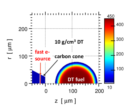
Figure 6: (Color online) Initial target density in g/cm³. The red line indicates the source cylinder where fast electrons are injected. The 8 g/cm³ carbon cone is colored blue for clarity.

The fast electron source was injected at $z=-20\,\mu$m with an intensity profile $I_{\mathrm{fast}}(r,t)=I_{0f}\exp\left[-(1/2)(r/r_{\mathrm{spot}})^{8}\right]f(t)$ with $f(t)$ a flattop from 0.5 to 18.5 ps with 0.5 ps linear ramps. Unless specified, we use $r_{\mathrm{spot}}=18\,\mu\mathrm{m}$. The total injected fast electron energy, $E_{\mathrm{fast}}$, is proportional to $I_{0f}$; in particular, for our runs, $E_{\mathrm{fast}}\mathrm{[kJ]}=I_{0f}/5.77\times 10^{18}$ W/cm². As discussed in Sec. II, we assume $I_{0f}$ is 0.52 times the laser intensity $I_{0L}$, which we need to find the ponderomotive temperature $T_{p}$ and energy spectrum. We consider a 527 nm (2nd harmonic of Nd:glass) laser wavelength, since this lowers $T_{p}\propto\lambda_{0}$ compared to first harmonic light (but is technologically more challenging).

IV.2 Results with artificially-collimated source

The fusion yield for the PIC-based energy spectrum and an artificially collimated source ($\Delta\theta=10^{\circ}$) is plotted against $E_{\mathrm{fast}}$ for several values of $r_{\mathrm{spot}}$ in Fig. 7. The points lie on a somewhat universal curve. This is due to two competing effects, both of which are discussed later in this section. First, the hot spots are in the “width $>$ depth” regime (Atzeni, Schiavi, and Bellei, 2007), where increasing the hot spot radius raises the required deposited heat for ignition. On the other hand, increasing the source area for fixed power decreases the energy of individual electrons, and leads to more effective stopping in the hot spot depth. We do not expect a strong dependence on $r_{\mathrm{spot}}$ for situations where source divergence has been mitigated. We use $r_{\mathrm{spot}}=18\,\mu$m in subsequent runs, since this ignites for the lowest $E_{\mathrm{fast}}$ of 132 kJ.

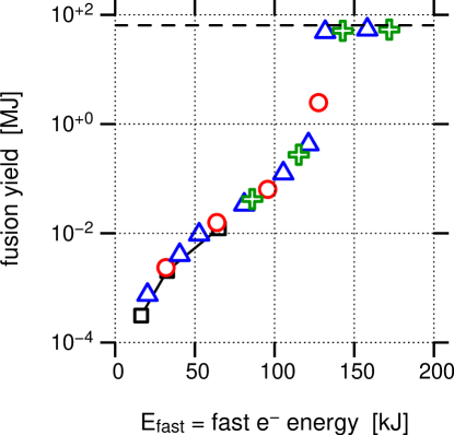
Figure 7: (Color online) Fusion yield vs. total injected fast electron energy, for Zuma-Hydra runs with an artificially collimated source $\Delta\theta=10^{\circ}$. $r_{\mathrm{spot}}=10\,\mu\mathrm{m}$ for black squares with solid line, 14 $\mu\mathrm{m}$ for red circles, 18 $\mu\mathrm{m}$ for blue triangles (case DQ10), and 23 $\mu\mathrm{m}$ for green crosses. In this and subsequent plots, the dashed black line at 64 MJ is the ideal fusion yield described in the text. The blue triangle with $E_{\mathrm{fast}}=132$ kJ is the lowest value that we deem to have ignited.

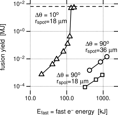
Figure 8: Fusion yield vs. total injected fast electron energy, for Zuma-Hydra runs for artificially collimated source $\Delta\theta=10^{\circ}$ with $r_{\mathrm{spot}}=18\,\mu\mathrm{m}$ (triangles, case DQ10), PIC-based source divergence $\Delta\theta=90^{\circ}$ with $r_{\mathrm{spot}}=18\,\mu\mathrm{m}$ (squares, case DQ90), and $\Delta\theta=90^{\circ}$ with $r_{\mathrm{spot}}=36\,\mu\mathrm{m}$ (circles, case DQ90_36).

For a collimated source, an estimate of the minimum ignition energy that must be delivered to the hot spot is given by Atzeni et al. in Ref. Atzeni, Schiavi, and Bellei, 2007. They performed 2D rad-hydro simulations of idealized, spherical fuel assemblies heated by a cylindrical beam of mono-energetic, forward-going particles which fully stop in a prescribed penetration depth. The result is

$$E_{\mathrm{ig}} = E_{\mathrm{opt}}F(\rho\Delta z,\rho r),$$ (16)

$$E_{\mathrm{opt}} = 140\left[\frac{\rho}{100\,\mathrm{g/cm}^{3}}\right]^{-1.85}\mathrm{kJ.}$$ (17)

$F>1$ if the hot spot transverse radius satisfies $\rho r>0.6$ g/cm² (“width $>$ depth” regime), or the depth satisfies $\rho\Delta z>\rho\Delta z_{\mathrm{opt}}=1.2$ g/cm². For our peak density of 450 g/cm³, $E_{\mathrm{opt}}=8.7$ kJ, and Atzeni finds an optimal hot-spot radius of $r_{\mathrm{opt}}=14\,\mu\mathrm{m}$ and pulse length of $t_{\mathrm{opt}}=15$ ps.

The minimum $E_{\mathrm{fast}}$ which ignited in the DQ10 series was 132 kJ, which is 15x $E_{\mathrm{opt}}$. We can understand this with the simplified runs listed at the top of Table I. First, DQ0 has a perfectly collimated source $(\Delta\theta=0)$, a mono-energetic 1.5 MeV spectrum, no angular scattering, and no E or B fields. This ignites for 18.4 kJ, or $2.1E_{\mathrm{opt}}$. This reflects our spot shape and temporal pulse being larger than Atzeni’s optimal values, and deposition in the low-density DT and carbon cone (which Atzeni did not include); we also did not optimize the 1.5 MeV source energy. The series DQ10_mono uses our small but nonzero $\Delta\theta=10^{\circ}$ and includes angular scattering, but no E or B fields; we now obtain ignition for $3.5E_{\mathrm{opt}}$. We adopt the PIC-based energy spectrum in DQ10_noEB but still include no E or B fields. This raises the ignition energy by another factor of 3.4, or $12E_{\mathrm{opt}}$. Finally, turning on E and B fields with the full Ohm’s law costs another 1.3x, bringing us to $15E_{\mathrm{opt}}$. The role of the energy spectrum and Ohm’s law for an artificially collimated source is discussed in more detail in (Strozzi et al., 2011).

We now estimate the effect of the PIC-based energy spectrum on ignition energy. Let $E_{\mathrm{stop}}$ be the energy delivered by a perfectly collimated beam with Atzeni’s optimal parameters to a hot spot of depth $\rho\Delta z_{\mathrm{opt}}$. The total fast electron energy $E_{\mathrm{fast}}=\alpha I_{0f}$ (with $\alpha=\pi r_{\mathrm{opt}}^{2}t_{\mathrm{opt}}$) is controlled by the fast electron intensity $I_{0f}$. We consider $\lambda_{0}=527$ nm and only collisional stopping (no angular scattering) of the fast electrons. The fraction of kinetic energy lost by a fast electron of kinetic energy $E$ in the hot spot is well fit by $f=\min(1,E_{DT}/E)$ where $E_{DT}=1.3$ MeV reflects the stopping in the DT hot spot. Integrated over our PIC-based energy spectrum, the ratio $E_{\mathrm{stop}}/E_{\mathrm{fast}}$ is approximately fit by

$$E_{\mathrm{stop}}/E_{\mathrm{fast}}\approx(1+I_{0f}/I_{0S})^{-0.48}\qquad I_{0S}=1.5\cdot 10^{19}\,\mathrm{W/cm^{2}}.$$ (18)

Figure 9 shows how these formulas apply to our PIC-based energy spectrum.

For $I_{0f}\gg I_{0S}$ , which our runs satisfy, we obtain

$$E_{\mathrm{stop}} \approx \alpha I_{0f}^{0.52}I_{0S}^{0.48},$$ (19)

$$E_{\mathrm{fast}} \approx \frac{E_{\mathrm{stop}}^{1.92}}{(\alpha I_{0S})^{0.92}}.$$ (20)

This is very close to what one finds with a ponderomotively-scaled energy spectrum by assuming all electrons lose $E_{DT}$:

$$E_{\mathrm{fast}}\approx\frac{E_{\mathrm{stop}}^{2}}{\alpha I_{0S}^{*}}\,\,\,\,\,\,\,\,\,\,I_{0S}^{*}\lambda_{0}^{2}=13.7\,\mathrm{GW}\frac{I_{0f}}{I_{0L}}\left[\frac{E_{DT}}{m_{e}c^{2}}\frac{T_{p}}{<E>}\right]^{2}.$$ (21)

Using the values found above for the bracketed quantities and $\lambda_{0}=527$ nm, we find $I_{0S}^{*}=1.6\times 10^{19}$ W/cm². This is very close to the fitted value given above. The upshot is that, due to partial stopping of fast electrons, the required short-pulse ignitor laser energy $\propto E_{\mathrm{fast}}$ scales roughly as square of the hot-spot energy. In addition, $E_{\mathrm{fast}}$ can be decreased by raising $I_{0S}$, which would happen if the electron stopping power were higher than our current value (e.g., due to micro-instabilities (Yabuuchi et al., 2009) or N-particle correlated stopping (Bret and Deutsch, 2008)).

From Eq. (18), achieving $E_{\mathrm{stop}}=E_{\textrm{{opt}}}$ of 8.7 kJ requires $E_{\mathrm{fast}}=5.6E_{\mathrm{stop}}=49$ kJ. This factor of 5.6x is 1.6 times larger than the 3.4x we found in going from case DQ10_mono to DQ10_noEB, which entailed going from the mono-energetic to PIC-based energy spectrum. We conjecture this is because DQ10_mono is already sub-optimal enough (ignites for $3.5E_{\mathrm{opt}}$) that we do not suffer the largest possible penalty for using the PIC-based energy spectrum. This implies more idealized targets like DQ0 would pay closer to the full penalty of 5.6x.

IV.3 Results with PIC-based, divergent source

Figure 8 presents the results for the cases DQ90 ($r_{\mathrm{spot}}=18\,\mu$m) and DQ90_36 ($r_{\mathrm{spot}}=36\,\mu$m) with the PIC-based source divergence $\Delta\theta=90^{\circ}$, as well as case DQ10 with an artificially collimated source of $\Delta\theta=10^{\circ}$. The PIC-based source is far from igniting, even for electron source energies $>$ 1 MJ. Figure 17 shows the greatly increased current divergence for DQ90. Note also the filaments that develop at large radius. Their nature and effect on beam propagation and fuel coupling should be further examined in future work. With the realistic divergence of $\Delta\theta=90^{\circ}$, the yield for the same $E_{\mathrm{fast}}$ is higher for the larger spot radius. This is generally the case for divergent sources, where the benefit of reduced laser intensity (and lower energy electrons, which stop more efficiently in the hot spot) outweighs the cost of increased spot size. Divergent sources thus ignite in the so-called “width $>$ depth regime”, where the hot spot has $\rho r$ above the optimal value of 0.6 g/cm². The source spot size that minimizes $E_{\mathrm{fast}}$ depends on details, like the cone-fuel standoff distance. In any case, its value will be unacceptably large for reactor purposes, so we turn our attention below to mitigating source divergence.

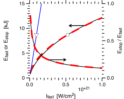
Figure 9: Fast electron coupling to optimal Atzeni hot spot described in text, with our PIC-based energy spectrum. Blue: total fast electron energy $E_{\mathrm{fast}}$. Solid black: exact $E_{\mathrm{stop}}(=E_{\mathrm{fast}}$ stopped in hot spot), and $E_{\mathrm{stop}}/E_{\mathrm{fast}}$ coupled to hot spot. Thick dashed red: approximate forms from Eq. (18). The triangle and square indicate points where $E_{\mathrm{stop}}$ equals the optimal ignition energy of 8.7 kJ.

V FAST ELECTRON confinement with imposed magnetic fields

We now attempt to recover the artificial-collimation 132 kJ ignition energy, with the realistic source divergence, by imposing various initial magnetic fields. This can be achieved with an axial field $B_{z}$ with no axial variation and strength $\sim$50 MG. However, axial variation in $B_{z}$ leads to a radial field $B_{r}$ and a $v\times B$ force in the $z$ direction (i.e., magnetic mirroring), as well as finite standoff distance from the source region to the confining field. We find that mirroring greatly reduces the benefit of magnetic fields. A magnetic pipe, with a $B_{z}$ that peaks at finite radius, does not suffer from the mirroring problem.

We wish to specify an arbitrary $B_{z}(r,z)$ in cylindrical coordinates, with no dependence on azimuth $\phi$. This can be accomplished by a vector potential $\vec{A}=A_{\phi}(r,z)\hat{\phi}$, which by construction satisfies the Coulomb gauge condition $\nabla\cdot\vec{A}=0$. The magnetic field $\vec{B}=\nabla\times\vec{A}$ automatically satisfies $\nabla\cdot\vec{B}=0$. In particular, $B_{z}=(1/r)\partial_{r}(rA_{\phi})$ and $B_{r}=-\partial_{z}A_{\phi}$. This allows us to solve for $A_{\phi}:$

$$A_{\phi}=\frac{1}{r}\int_{0}^{r}dr^{\prime}\,r^{\prime}B_{z}(r^{\prime},z).$$ (22)

As $r\rightarrow 0$, if $B_{z}\rightarrow kr^{p}$ then $A_{\phi}\rightarrow k(p+2)^{-1}r^{p+1}$. Since $B_{r}$ scales with $r$ like $A_{\phi}$, as long as $p\geq-1$, Eq. (22) guarantees $B_{r}(r=0)=0$. This is physically necessary, since the radial direction is ill-defined at $r=0$. We can find the current $\vec{J}=J_{\phi}\hat{\phi}$ needed to maintain the magnetic field from Ampère’s law without displacement current:

$$\mu_{0}J_{\phi}=\partial_{z}B_{r}-\partial_{r}B_{z}=\nabla^{2}(A_{\phi}\hat{\phi)}.$$ (23)

We estimate the magnitude of $J_{\phi}\sim B/\mu_{0}L$, and taking $B\sim 10$ MG, $L\sim 10\,\mu\mathrm{m}$ gives $J_{\phi}\sim 10^{14}$ A/m². The fast electron current is of order $n_{cr}ec$, which for 527 nm light is $1.9\times 10^{17}$ A/m². Although substantial, the currents implied by our imposed fields are much less than the fast electron current. They may compete with the much smaller net (fast plus background) current.

V.1 High $B_{z}$ in fast electron source region

We utilize initial magnetic fields of the form

$$B_{z}=B_{z0}+(B_{z1}-B_{z0})H(z)\exp\left[-\left((r-r_{0})/\Delta r\right)^{8}\right].$$ (24)

Except for the magnetic pipe configurations discussed below, $r_{0}=0$ and $\Delta r=50\,\mu$m. We first consider a $B_{z}$ that we call “uniform,” since it does not vary between the source region and dense fuel. $B_{z}(z)$ for several cases is plotted in Fig. 11. For the uniform case, $H(z)=1$ for $z<80\,\mu\mathrm{m}$, with a piecewise-parabolic ramp to zero for $z>110\,\mu\mathrm{m}$. $B_{z0}=0.1$ MG is the uncompressed seed field, and we vary the peak compressed field $B_{z1}$. Setting $H=1$ slightly decreases the ignition energy, but may be less realistic than our $H(z)$. Figure 10 shows the fusion yield for the PIC-based source divergence ($\Delta\theta=90^{\circ})$ and various values of $B_{z1}$. An initial field of $B_{z1}=10$ MG gives better coupling than the unmagnetized cases, but would still lead to an unacceptable ignition energy. A field of 30 MG (case BZ30) gives about 2x the ignition energy as an artificially collimated source ($\Delta\theta=10^{\circ})$, while 50 MG (case BZ50) gives essentially the same coupling.

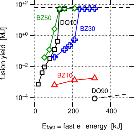
Figure 10: (Color online) Fusion yield for runs with $r_{\mathrm{spot}}=18\,\mu\mathrm{m}$. Black solid line with squares is for an artificially collimated source $\Delta\theta=10^{\circ}$ (case DQ10). All other cases use the PIC-based source divergence ($\Delta\theta=90^{\circ})$. Black dashed line with circles is for no imposed B field (case DQ10_18). The other cases have a “uniform” initial $B_{z}$ given by Eq. (24), with $B_{z1}=10$ MG (red triangles), 30 MG (blue crosses, case BZ30), and 50 MG (green diamonds, case BZ50).

The pressure and fast electron current profiles in Fig. 17 illustrate the improvement due to the imposed field. The current is much more confined in the case BZ50 than without the field, although not as much as in the artificial-collimation case DQ10. The loss of confinement at $z\approx 100\,\mu\mathrm{m}$ is due to the end of the high-field region (see Fig. 11). Note also the appearance of current to the left of the fast electron injection plane at $z=-20\,\mu\mathrm{m}$. We call this the reflected current. It is due to the plasma being slightly diamagnetic, and reducing the imposed $B_{z}$ somewhat during the course of the run. The reflected current becomes enhanced in runs with significant mirroring, such as case BZ0-50.

We now turn to the effect of more realistic initial field geometries. It is plausible to compress the field to the desired strength, $\gtrsim$50 MG, in a fast-ignition fuel-assembly implosion (Tabak et al., 2010). However, it will not be uniform. In particular, to the extent the MHD frozen-in law is followed, the axial field compression will follow the radial compression of matter. Standard schemes of fuel assembly around a cone tip will thus result in the largest field being located between the cone tip and dense fuel. Moreover, the purpose of the cone is to provide a plasma-free region so the short-pulse laser converts to fast electrons near the fuel. The shell motion down the outer cone surface launches a strong shock in the cone, which must not reach the inner cone surface before the short-pulse laser fires (to avoid a rarefaction that would fill the cone interior). In standard schemes, the short-pulse laser thus converts to fast electrons in a region with essentially the uncompressed, seed magnetic field. The field may be enhanced somewhat by resistive diffusion of compressed field into and through the cone material, but we expect the cone and surrounding DT to be sufficiently conducting to prevent significant diffusion.

The upshot is the fast electrons must transit from their birth region of low field to a region of high field in front of the cone. This poses two separate challenges. First, the fast electrons may be reflected axially by the magnetic mirror effect. Also, they must travel a finite standoff distance before the compressed field can impede their radial motion.

We consider the role of mirroring with no standoff, by modifying $H(z)$. We first increase $B_{z}$ to 75 MG at $z=30\,\mu\mathrm{m}$ (located between the cone tip and the dense fuel) while keeping $B_{z}$ fixed at 30 MG (case BZ30-75) or 50 MG (case BZ50-75) in the source region. The new $B_{z}$ profiles are plotted in Fig. 11. Table I and Fig. 12 show that the energy needed to ignite increases slightly for case BZ50-75 but substantially for case BZ30-75. This demonstrates the significant impact of mirroring for modest (1.5-2.5x) increases in $B_{z}$ between the source and fuel regions.

To demonstrate further the impact of mirroring, we plot in Fig. 13 the reflected fraction, or the ratio of the fast electron energy reaching the left edge of the domain ($z=-50\,\mu\mathrm{m})$ to $E_{\mathrm{fast}}$. For fixed $E_{\mathrm{fast}}$, the reflected fraction is quite small for the uniform field profiles, but substantial for the non-uniform ones. The reflected fraction actually understates the effect of mirroring. The low-energy electrons deposit more of their energy in the hot spot, and are also more magnetized (and thus more likely to mirror). So, the reflected electrons would have more effectively heated the hot spot than typical electrons.

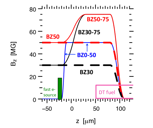
Figure 11: (Color online) $B_{z}$ profiles at $r=0$. Thick black dash: case BZ30, thick red dash: case BZ50, black solid: case BZ30-75, red solid: case BZ50-75, blue solid: case BZ0-50.

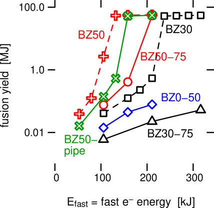
Figure 12: (Color online) Fusion yield for runs from Fig. 11. The curves have the same meaning as in that figure. solid green X’s is case BZ50pipe. The other curves have the same meaning as in Fig. 11: black dash squares: case BZ30, red dash crosses: case BZ50, black solid triangles: case BZ30-75, red solid circles: case BZ50-75, blue solid diamonds: case BZ0-50.

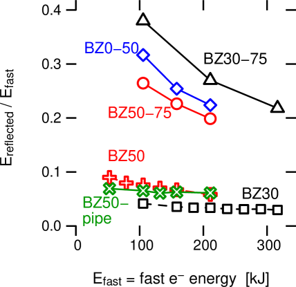
Figure 13: (Color online) Reflected fraction, i.e. the fast electron energy reaching left $z$ boundary, divided by $E_{\mathrm{fast}}$. The runs and curves are as in Fig. 12: solid green X’s: case BZ50pipe, black dash squares: case BZ30, red dash crosses: case BZ50, black solid triangles: case BZ30-75, red solid circles: case BZ50-75, blue solid diamonds: case BZ0-50.

V.2 Low $B_{z}$ in fast electron source region: the magnetic pipe

We now turn to the situation where the fast electrons are born in the uncompressed seed field. First we consider case BZ0-50, where the field rises quickly in $z$, so that standoff is minimized. Figure 11 shows the $B_{z}$ profile. The electrons are still subject to the mirror force, which results in an ignition energy of $E_{\mathrm{fast}}>211$ kJ (blue curve in Fig. 12). Runs with higher $E_{\mathrm{fast}}$ encountered numerical difficulties, which we are studying. Figure 13 depicts the reflected fraction, indicating substantial mirroring in this case. Figure 17 shows the increase in the reflected current in case BZ0-50 compared to BZ50.

To remedy mirroring, we propose a hollow magnetic pipe, which is free of high field at small radius. Fast electrons are reflected by the pipe as they move outward radially, but do not experience a mirror force in $z$ ($\partial_{z}B_{z}=B_{r}=0$ inside the pipe). A certain product of field strength times length is needed to reflect an electron, and can be estimated for planar (not cylindrical) geometry by (Robinson and Sherlock, 2007)

$$BL>K\gamma\beta(1-\cos\theta),\qquad\qquad K\equiv\frac{m_{e}c}{e}=17.0\,\mathrm{MG}\cdot\mu\mathrm{m}.$$ (25)

For our PIC-based $\Delta\theta=90^{\circ}$ angle spectrum, $\left\langle 1-\cos\theta\right\rangle=0.43$. The ignition energy for case DQ10 (artificial collimation) was 132 kJ, which gives an average electron energy of 8.5 MeV. This requires $BL>129$ MG$\cdot\mu$m to reflect. Although lower-energy particles are easier to reflect and stop more fully in the DT hot spot, our spectrum does not contain much energy there. For $B=50$ MG, we need a pipe of thickness 2.6 $\mu$m. We consider pipes that are thicker than this, which substantially reduce the ignition energy over the no-field case. The results shown here establish the feasibility of the pipe. We are exploring thinner, more optimal pipes, which entails variation of other parameters like spot size.

The initial field for the case BZ50pipe is given by Eq. (24) with $r_{0}=35\,\mu$m and $\Delta r=15\,\mu$m, and is displayed in Fig. 14. This gives roughly the same ignition energy as the uniform $B_{z}$ field, shown as the solid green line in Fig. 12. The mirror effect, as measured by the reflected fraction, is about the same as for the uniform case BZ50 (see Fig. 13). We studied pipes with a peak field of 30 and 50 MG (cases BZ30pipe and BZ50pipe), as well as thin and thick 50 MG pipes (cases BZ50pipe and BZ50pipeA, see Fig. 16).

We summarize the development of this paper in Fig. 15. The challenge was to find imposed magnetic field configurations that recover the performance of an artificially collimated fast electron source, when using the PIC-based divergent source. A uniform 50 MG axial field does this, and may even perform slightly better. However, the more realistic case is for fast electrons to be born in a lower field and suffer magnetic mirror forces. To circumvent this, we introduced the hollow magnetic pipe. For a 50 MG peak field, this works essentially as well as the uniform field. A lower peak field of 30 MG performs significantly worse than the 50 MG cases, for both the uniform and pipe configurations.

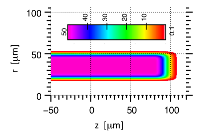
Figure 14: (Color online) Initial $B_{z}$ profile, in MG, for case BZ50pipe.

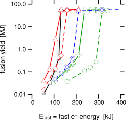
Figure 15: (Color online) Fusion yield for run cases DQ10 (solid black squares), BZ50 (solid red triangles), BZ50pipe (dashed red diamonds), BZ50pipeA (dashed blue X’s) BZ30 (solid green crosses), and BZ30pipe (dashed green circles).

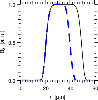
Figure 16: (Color online) Radial $B_{z}$ profiles for pipe cases BZ30pipe and BZ50pipe (solid black), and BZ50pipeA (thick dashed blue).

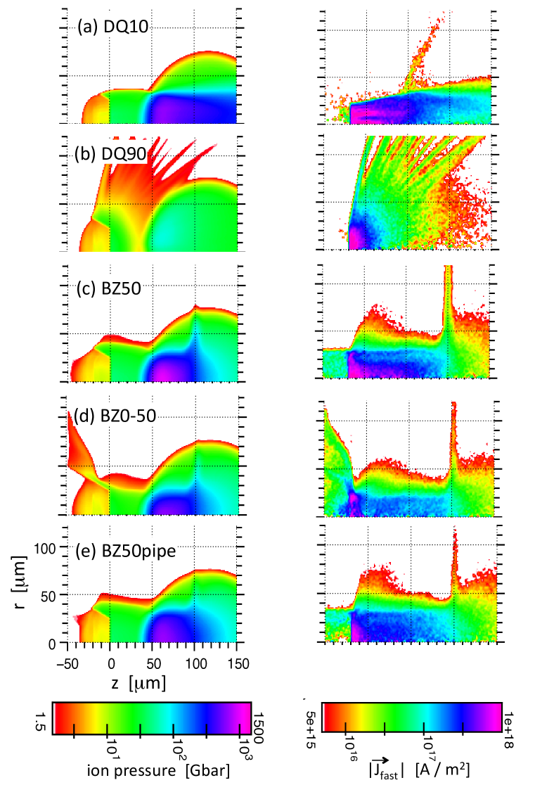
Figure 17: (Color online) Ion pressure (left) and fast electron current density $|\overrightarrow{J}_{\mathrm{fast}}|$ (right) at time 10 ps (middle of fast electron time pulse) for cases, from top to bottom: DQ10, DQ90, BZ50, BZ0-50, and BZ50pipe. All cases have $E_{\mathrm{fast}}=158$ kJ, except DQ90 has $E_{\mathrm{fast}}=317$ kJ.

VI Conclusion

In this paper, we have presented recent transport modeling efforts geared towards a fast ignition “point design.” This requires knowledge of the fast electron source produced by a short-pulse laser. We characterized the results of a full-PIC 3D simulation with the PSC code in terms of 1D energy and angle spectra. The energy spectrum is well-matched by a quasi two-temperature form, which we scale ponderomotively as we vary $I\lambda^{2}$. The angle spectrum is divergent, and the PIC data showed only a slight reduction in average angle with electron energy (justifying our 1D factorization). A more sophisticated handoff method involving a 4D distribution function, and using more recent PIC simulations, seems to give qualitatively similar results . The major design challenges posed by this source are: 1. the electrons are too energetic to fully stop in a DT hot spot, and 2. they are sufficiently divergent that mitigation strategies are required in a point design.

We have developed a transport modeling capability which entails the hybrid-PIC code Zuma and rad-hydro code Hydra running in tandem. We detailed the physics contained in Zuma. It is similar to other codes that use a reduced model to eliminate light and Langmuir waves. Namely, the displacement current is removed from Ampère’s law, and the electric field is found from Ohm’s law (obtained from the background electron momentum equation). This model is applicable in sufficiently collisional plasmas, and for time and space scales longer than the plasma frequency and Debye length.

Zuma-Hydra 2D cylindrical RZ runs on an idealized cone-fuel assembly were performed. For a perfectly parallel source ($\Delta\theta=0$, no angular scattering) of mono-energetic 1.5 MeV electrons, ignition occurred for 18.5 kJ of fast electrons, or 2.1x Atzeni’s ideal estimate of 8.7 kJ. We discussed the impact of (small) divergence, E and B fields, and the PIC-based energy spectrum, and refer the reader to Ref. Strozzi et al., 2011 for more details, including the role of different terms in Ohm’s law. With the PIC-based energy spectrum, the full Ohm’s law, and an artificially-collimated source ($\Delta\theta=10^{\circ}$), the ignition energy was raised to 132 kJ, or 15x the ideal value.

The realistic angular spectrum was then considered, and raised the ignition energy to $>$ 1 MJ. Several mitigation ideas have been proposed, including magnetic fields produced by resistivity gradients (e.g. at material interfaces). While this approach is promising, we chose to examine imposed axial magnetic fields. An initial, uniform field of 50 MG recovered the 132 kJ ignition energy of the artificially collimated source. Assembling $\sim 10$’s MG field strengths in an ICF implosion, via the frozen-in law of MHD, is reasonable, and has been demonstrated recently at Omega.

However, a cone-in-shell implosion is not likely to produce a uniform magnetic field. In particular, the field in the fast electron source region (inside the cone tip) will not be enhanced much over the seed value, but would be enhanced in the region between the cone tip and dense fuel (Tabak et al., 2010). Fast electrons would therefore encounter an increasing axial field, and be subject to magnetic mirroring. Simulations that quantify this effect for a few profiles were shown. We showed one way to provide confinement but avoid mirroring is a magnetic pipe, which peaks at a finite radius.

We have started to address the design problem of assembling a pipe field in an implosion. Inserting an axial structure (a “wire”) between the cone tip and fuel, that does not get compressed, is one way to achieve this. Magnetic confinement schemes based on self-generated azimuthal fields due to resistivity gradients require a similar structure. Thus both approaches share some hydro assembly features, and would mutually benefit from progress in hydro design. One advantage of the pipe in this regard is that the resistivity (e.g., Z) is irrelevant for the pipe, as long as it isn’t compressed and thereby produce a large on-axis field. The self-azimuthal fields rely on resistivity gradients, usually achieved by a high-Z material on-axis. This can lead to unacceptable fast-electron energy loss or angular scattering in the wire . Megagauss magnetic fields may lower the ignition threshold by reducing electron thermal conduction out of the hot spot or, at even higher values, enhancing alpha deposition.

Integrated hybrid-PIC and rad-hydro simulations offer a powerful new tool for fast-ignition modeling, and we look forward to them enabling the emergence of attractive ignition designs.