The Peregrine rogue waves induced by interaction between the continuous wave and soliton

Abstract

Based on the soliton solution on a continuous wave background for an integrable Hirota equation, the reduction mechanism and the characteristics of the Peregrine rogue wave in the propagation of femtosecond pulses of optical fiber are discussed. The results show that there exist two processes of the formation of the Peregrine rogue wave: one is the localized process of the continuous wave background, and the other is the reduction process of the periodization of the bright soliton. The characteristics of the Peregrine rogue wave are exhibited by strong temporal and spatial localization. Also, various initial excitations of the Peregrine rogue wave are performed and the results show that the Peregrine rogue wave can be excited by a small localized (single peak) perturbation pulse of the continuous wave background, even for the nonintegrable case. The numerical simulations show that the Peregrine rogue wave is unstable. Finally, through a realistic example, the influence of the self-frequency shift to the dynamics of the Peregrine rogue wave is discussed. The results show that in the absence of the self-frequency shift, the Peregrine rogue wave can split into several subpuslses; however, when the self-frequency shift is considered, the Peregrine rogue wave no longer splits and exhibits mainly a peak changing and an increasing evolution property of the field amplitude.

I Introduction

A rogue wave is an oceanic phenomenon with amplitude much higher than the average wave crests around them Kharif_Book . So far, this phenomenon has not been understood completely due to the difficult and restricted observational conditions. Therefore a great deal of attention has been paid to better understanding their physical mechanisms. It has been suggested that the rogue waves appearing in the ocean are mainly caused by wave-wave nonlinear interaction, such as a modulation instability of the Benjamin-Feir type Kharif ; Ruban ; Andonowati ; Zakharov ; Slunyaev . Recently, rogue waves have been observed in optical fibers Solli1 , in superfluid helium Ganshin , and in capillary waves Shats , respectively. These discoveries indicate that rogue waves may be rather universal. Certainly, we cannot harness the occurrence of rogue waves in the ocean due to their enormous destructiveness. In optics, however, the optical rogue waves produced in supercontinuum generation can be used to generate highly energetic optical pulses Solli1 ; Dudley ; Mussot ; Solli3 ; Taki .

Deep waves in the ocean and the wave propagation in optical fibers can be described by the nonlinear Schrödinger (NLS) equation. Based on the model, the rogue wave phenomenon has been extensively studied, including rational solutions and their interactions Osborne ; Osborne2 ; Akhmediev1 ; Akhmediev2 ; Akhmediev3 ; Akhmediev4 ; Ankiewicz1 ; Yan , pulse splitting induced by higher-order modulation instability, and wave turbulence Erkintalo ; Kibler . A fundamental analytical solution on the rogue waves is the Peregrine solution (PS), which was first presented by Peregrine Peregrine . PS is a localized solution in both time and space, and is a limiting case of Kuznetsov-Ma solitons Kuznetsov ; Ma and Akhmediev breathers Akhmediev8 . Recently, the excitation conditions of PS have been demonstrated experimentally in optical fiber, and explicitly characterized its two-dimensional localization NatPhys ; Hammani . It should be noted that the results are theoretically described by the NLS equation, which is valid for the picosecond pulses. When describing the characteristics of PS in the femtosecond regime, we must consider some higher-order effects, such as third-order dispersion (TOD), self-steepening and self-frequency shift, and so on. In this case, we should consider the higher-order nonlinear Schrödinger (HNLS) equation in the form Kodama

$$\frac{\partial q}{\partial z} =i\left(\alpha_{1}\frac{\partial^{2}q}{\partial t^{2}}+\alpha_{2}\left|q\right|^{2}q\right)+\alpha_{3}\frac{\partial^{3}q}{\partial t^{3}}$$

$$+\alpha_{4}\frac{\partial\left|q\right|^{2}q}{\partial t}+\alpha_{5}q\frac{\partial\left|q\right|^{2}}{\partial t},$$ (1)

where $q(z,t)$ is the slowly varying envelope of the electric field, $z$ and $t$ denote normalized propagation distance and the retarded temporal coordinate, respectively, and the parameters $\alpha_{1},\alpha_{2},\alpha_{3},\alpha_{4},$ and $\alpha_{5}$ are the real constants related to the group velocity dispersion (GVD), the self-phase modulation (SPM), the third-order dispersion (TOD), the self-steepening and the delayed nonlinear response effect, respectively.

Generally, the HNLS equation (1) is not integrable. To solve Eq (1), we first consider the special parametric choice with $\alpha_{2}=2\mu^{2}\alpha_{1}$, $\alpha_{4}=$ $6\mu^{2}\alpha_{3},$ $\alpha_{4}+\alpha_{5}=0$ so that Eq. (1) becomes Hirota

$$\frac{\partial q}{\partial z}=i\left(\alpha_{1}\frac{\partial^{2}q}{\partial t^{2}}+\alpha_{2}\left|q\right|^{2}q\right)+\alpha_{3}\frac{\partial^{3}q}{\partial t^{3}}+\alpha_{4}\left|q\right|^{2}\frac{\partial q}{\partial t},$$ (2)

which is usually called the Hirota equation, where the parameter $\mu$ is a real constant.

The equation was first presented by Hirota Hirota , and subsequently many researchers analyzed this equation from different points of view Lakshmanan ; Mihalache1 ; Mihalache2 ; Porsezian ; Mihalache3 ; Li ; Xu ; lishuqing . Recently, the rogue waves and the rational solutions of the Hirota equation have been discussed in the forms of the two lower-order solutions by employing the Darboux transformation technique Ankiewicz2 . In this paper, based on the soliton solution on a continuous wave (CW) background for the integrable Hirota equation (2), we discuss the formation mechanism and the characteristics of the PS in the femtosecond regime. The results show that the PS exhibits a feature of temporal and spatial localization and can be excited by a small localized (single peak) perturbation pulse of the CW background, even for the nonintegrable HNLS equation (1). Based on this result, we discuss the dynamics of the Peregrine rogue wave through a realistic example.

The paper is organized as follows. In Sec. II we present the explicit process of the formation of the PS from the Kuznetsov-Ma solitons and Akhmediev breathers based on the soliton solution on a CW background for the Hirota equation and discuss the characteristics of the PS. Various initial excitations of the PS are discussed in Sec. III. Subsequently, in Sec. IV we investigate the influence of the self-frequency shift to the dynamics of the Peregrine rogue wave by employing a realistic example. Our results are summarized in Sec. V.

II The Peregrine solution induced by interaction between the continuous wave background and soliton

By employing a Darboux transformation, one can construct the soliton solution on a CW background for Eq. (2) as follows Xu ; lishuqing

$$q(z,t) =\left(A+A_{s}\frac{a\cosh\theta+\cos\varphi}{\cosh\theta+a\cos\varphi}\right.$$

$$\text{ \ \ }\left.+iA_{s}\frac{b\sinh\theta+c\sin\varphi}{\cosh\theta+a\cos\varphi}\right)\exp\left(i\varphi_{c}\right).$$ (3)

Here

$$\theta =M_{I}T-\left(\nu_{1}M_{R}+\nu_{2}M_{I}\right)Z,$$

$$\varphi =M_{R}T-\left(\nu_{2}M_{R}-\nu_{1}M_{I}\right)Z,$$

$$\varphi_{c} =\omega T+\left[(2\mu^{2}A^{2}-\omega^{2})\alpha_{1}+\omega(6\mu^{2}A^{2}-\omega^{2})\alpha_{3}\right]Z,$$

with $T=t-t_{0}$, $Z=z-z_{0}$, and the coefficients are $a=-2\mu^{2}AA_{s}/(\mu^{2}A_{s}^{2}+M_{R}^{2})$, $b=-2\mu AM_{R}/(\mu^{2}A_{s}^{2}+M_{R}^{2})$, and $c=M_{I}/(\mu A_{s})$, which implies that $M_{I}=0$ as $A_{s}=0$. And other coefficients $\nu_{1}=\mu A_{s}[\alpha_{1}+(\omega+2\omega_{s})\alpha_{3}]$, $\nu_{2}=(\omega+\omega_{s})\alpha_{1}+(\omega^{2}+\omega\omega_{s}+\omega_{s}^{2}-2\mu^{2}A^{2}-\mu^{2}A_{s}^{2})\alpha_{3}$, $M_{R}=\{[((\omega_{s}-\omega)^{2}+\allowbreak 4\mu^{2}A^{2}-\mu^{2}A_{s}^{2})^{2}+4\mu^{2}A_{s}^{2}(\omega_{s}-\omega)^{2}]^{1/2}+((\omega_{s}-\omega)^{2}+4\mu^{2}A^{2}-\mu^{2}A_{s}^{2})\}^{1/2}/\sqrt{2}$, and $M_{I}=\{[((\omega_{s}-\omega)^{2}+\allowbreak 4\mu^{2}A^{2}-\mu^{2}A_{s}^{2})^{2}+4\mu^{2}A_{s}^{2}(\omega_{s}-\omega)^{2}]^{1/2}-((\omega_{s}-\omega)^{2}+4\mu^{2}A^{2}-\mu^{2}A_{s}^{2})\}^{1/2}/\sqrt{2}$, and $t_{0}$, $z_{0}$, $A$, $\omega$, $A_{s}$, and $\omega_{s}$ are the arbitrary real constants, and without loss of generality we assume that $A$ and $A_{s}$ are non-negative constants. The solution (3) includes two special cases. One is that as the amplitude $A$ vanishes, it reduces to the solution $q_{s}(z,t)=A_{s}e^{i\varphi_{s}}\operatorname{sech}\theta$, where $\theta=\mu A_{s}T-\mu A_{s}[2\omega_{s}\alpha_{1}+(3\omega_{s}^{2}-\mu^{2}A_{s}^{2})\alpha_{3}]Z$ and $\varphi_{s}=\varphi_{c}+\varphi=\omega_{s}T+[\left(\mu^{2}A_{s}^{2}-\omega_{s}^{2}\right)\alpha_{1}+\omega_{s}(3\mu^{2}A_{s}^{2}-\omega_{s}^{2})\alpha_{3}]Z$, which describes a bright soliton solution with the maximal amplitude $A_{s}$. The other is that when the soliton amplitude $A_{s}$ vanishes, it reduces to the CW light solution $q_{c}(z,t)=Ae^{i\varphi_{c}}$. Therefore, in general, the exact solution $q(z,t)$ in Eq. (3) describes a soliton solution embedded in a CW light background with the group velocity $V_{sc}=(\nu_{1}M_{R}+\nu_{2}M_{I})/M_{I}$ lishuqing . Specifically, when $\alpha_{3}=0$ and taking $\alpha_{1}=-1$, $\mu=1$, the solution (3) coincides with the result given in Ref. Park , which is firstly derived from NLS equation by N. Akhmediev and V. I. Korneev Akhmediev8 .

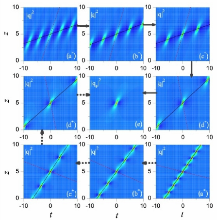
Figure 1: (Color online) The reduction process from the solution (3) to the Peregrine solution (4) as $(A_{s},\omega_{s})\rightarrow(2A^{\mp},\omega)$. (a^-) $A_{s}=A$, $\omega_{s}=0.6\omega$; (b^-) $A_{s}=1.45A$, $\omega_{s}=0.7\omega$; (c^-) $A_{s}=1.6A$, $\omega_{s}=0.8\omega$; (d^-) $A_{s}=1.99A$, $\omega_{s}=0.85\omega$; (a⁺) $A_{s}=3A$, $\omega_{s}=1.4\omega$; (b⁺) $A_{s}=2.5A$, $\omega_{s}=1.3\omega$; (c⁺) $A_{s}=2.4A$, $\omega_{s}=1.2\omega$; (d⁺) $A_{s}=2.01A$, $\omega_{s}=1.15\omega$; and (e) the Peregrine solution given by (4) with $A_{s}=2A$ and $\omega_{s}=\omega$. The slope of red dashed lines is $K_{\varphi}$, and black solid lines is $K_{\theta}$. Here the parameters are $A=1$, $\omega=1$, $t_{0}=0$, $z_{0}=5$, $\mu=1$, $\alpha_{1}=0.5$, and $\alpha_{3}=0.05$.

In the limit $(A_{s},\omega_{s})\rightarrow(2A,\omega)$, Eq. (3) reduces to PS as follows

$$q_{\text{p}}(z,t)=Ae^{i\varphi_{c}}\left[\frac{4+i8CZ}{1+4C^{2}Z^{2}+4B^{2}\left(T-DZ\right)^{2}}-1\right],$$ (4)

where $B=\mu A$, $C=2B^{2}(\alpha_{1}+3\omega\alpha_{3})$ and $D=2\omega\alpha_{1}+3(\omega^{2}-2B^{2})\alpha_{3}$, which is a rational fraction solution, and is first derived from the Kuznetsov-Ma breather (KMB) by Peregrine Peregrine ; Kuznetsov ; Ma and so is called the Peregrine solution or the Peregrine rogue wave (Note that it is regarded as the Peregrine soliton in Refs. NatPhys ; Hammani .) Here $(t_{0},z_{0})$ presents the peak position of the PS. In order to understand the characteristics of the solution (3), Fig. 1 presents the reduced process from the solutions (3) to the PS (4) as $(A_{s},\omega_{s})\rightarrow(2A^{-},\omega)$ and $(A_{s},\omega_{s})\rightarrow(2A^{+},\omega)$, respectively. From them one can see directly that the solution (3) commonly exhibits breather characteristics, and the separation between adjacent peaks gradually increases as $(A_{s},\omega_{s})\rightarrow(2A,\omega)$, and eventually reduces into the PS. The most impressive feature on the PS is localized in both time and space. The peak position of the PS is fixed at spatiotemporal position $z=z_{0}$ and $t=t_{0}$ during the reduction, and the peak power $|q_{\text{p}}(z_{0},t_{0})|^{2}=(A+A_{s})^{2}\rightarrow 9A^{2}$ as $A_{s}\rightarrow 2A$, which means that the PS with peak power $9A^{2}$ can be generated by choosing an initial excitation properly.

It should be pointed out that in the reduction process mentioned above, the physical mechanism for the formation of the PS has some differences. Figures 1(a^-)–1(e) demonstrate a localized process of CW background along the slope direction $K_{\varphi}=M_{R}/(\nu_{2}M_{R}-\nu_{1}M_{I})$, while Figs. 1(a⁺)–1(e) show a periodization process of bright soliton along the slope direction $K_{\theta}=M_{I}/(\nu_{1}M_{R}+\nu_{2}M_{I})$. Furthermore, Fig. 2 presents the contour plots of $K_{\theta}$ and $K_{\varphi}$ as a function of $A_{s}$ and $\omega_{s}$ for given $A$ and $\omega$. Note that $K_{\varphi}$ is infinite as $\nu_{2}M_{R}-\nu_{1}M_{I}=0$ except for the point $(2A,\omega)$, which corresponds to the line $t=t_{0}$ and appears at the sixth curve in Fig. 2(b). When $(A_{s},\omega_{s})\rightarrow(2A,\omega)$, the limitations of $K_{\varphi}$ and $K_{\theta}$ do not exist, and at this point the solution is localized along both slope directions $K_{\varphi}$ and $K_{\theta}$, namely, the PS appears. Therefore, the PS should be a middle state in the process of the localization of CW converting into the periodization of the bright soliton, as shown in Ref. Akhmediev3 .

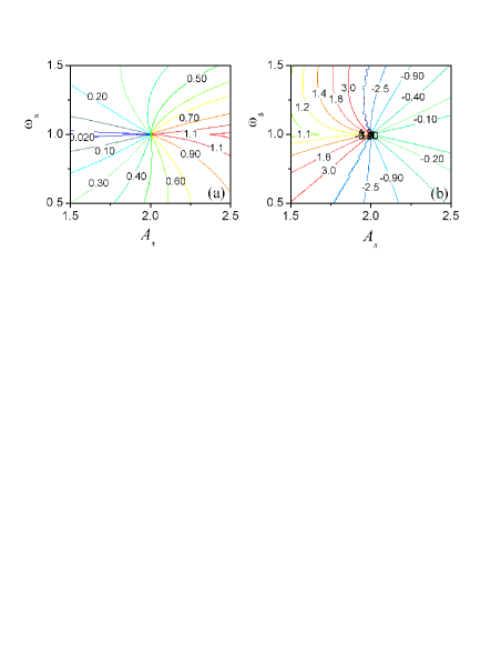
Figure 2: (Color online) The contour plots of (a) $K_{\theta}$ and (b) $K_{\varphi}$ as a function of $A_{s}$ and $\omega_{s}$, where the parameters are $A=1$, $\omega=1$, $\mu=1$, $\alpha_{1}=0.5$, and $\alpha_{3}=0.05$, and the contour values (from left to right) are $0.02,$ $0.1$, $0.2$, $0.3$, $0.4$, $0.5$, $0.6$, $0.7$, $0.9$, $1.1$, $1.3$ in (a), and the contour values are $1.1$, $1.2$, $1.4$, $1.8$, $3$, $-2.5$, $-0.9$, $-0.4$, $-0.2$, $-0.1$ in (b), respectively.

In order to understand better the reduction processes of the PS, we consider a special case for the solution (3) with $\omega_{s}=\omega$. In this case, the solution (3) has two different expressions. When $A_{s}^{2}<4A^{2}$, the solution (3) can be written as

$$q(z,t)=\left(\Omega_{R}\frac{\Omega_{R}\cosh\theta+iA_{s}\sinh\theta}{2A\cosh\theta-A_{s}\cos\varphi}-A\right)e^{i\varphi_{c}},$$ (5)

where $\theta=\mu^{2}A_{s}\Omega_{R}(\alpha_{1}+3\omega\alpha_{3})Z$ and $\varphi=\mu\Omega_{R}T-\mu\Omega_{R}[2\omega\alpha_{1}+(3\omega^{2}-2\mu^{2}A^{2}-\mu^{2}A_{s}^{2})\alpha_{3}]Z$ with $\Omega_{R}=\sqrt{4A^{2}-A_{s}^{2}}$ being a modulation frequency. Here $K_{\theta}=0$ and $K_{\varphi}=1/[2\omega\alpha_{1}+(3\omega^{2}-2\mu^{2}A^{2}-\mu^{2}A_{s}^{2})\alpha_{3}]$. Therefore the solution (5) is periodic with period $t_{\text{per}}=2\pi/(\mu\Omega_{R})$ along the $t$ axis and localized along the $z$ axis, and is usually called an Akhmediev breather (AB), which can be considered as a modulation instability process Ablowitz . In this case, the solution (5) can reduce to the CW background $q_{c}(z,t)$ as $A_{s}\rightarrow 0$, and with the increasing of $A_{s}$ the CW background is gradually localized due to the interaction with the soliton and forms a periodic breather with period $t_{\text{per}}$, i. e, the AB [see Fig. 3(a)], eventually when $A_{s}$ tends to $2A$, the solution (5) becomes the PS. This process represents the reduction of CW$\rightarrow$AB$\rightarrow$PS. Also, it can be described by the ratio between the period $t_{\text{per}}$ and the temporal width $\delta t_{0}$ as follows:

$$\frac{t_{\text{per}}}{\delta t_{0}}=\frac{2\pi}{\cos^{-1}\left(\frac{A_{s}}{A}-2\frac{A}{A_{s}}\right)},$$ (6)

where the temporal width $\delta t_{0}$ is defined as the width from zero-value of intensity to adjacent peak NatPhys . Figure 3(b) presents the dependence of the ratio $t_{\text{per}}/\delta t_{0}$ on $A_{s}/A$. From it, one can see that when $A_{s}/A$ approaches $2$, the ratio $t_{\text{per}}/\delta t_{0}$ tends to infinity, which implies that the separation between peaks is more and more large, eventually resulting in the localization along the $t$ axis, and forms the PS. From the expression (6), one can see that this process does not depend on the higher-order parameter $\alpha_{3}$, which means that when the higher-order effects with the conditions $\alpha_{2}=2\mu^{2}\alpha_{1}$, $\alpha_{4}=$ $6\mu^{2}\alpha_{3}$, and $\alpha_{4}+\alpha_{5}=0$ simultaneously appear in the optical fiber, they do not influence the characteristics of the PS. It should be emphasized that the Peregrine solution generated by the process of the reduction of CW$\rightarrow$AB$\rightarrow$PS has been already studied theoretically and experimentally in the framework of the NLS equation Osborne ; Akhmediev3 ; Ma ; Akhmediev8 ; NatPhys ; Hammani . Here we presented the corresponding descriptions in the femtosecond regime.

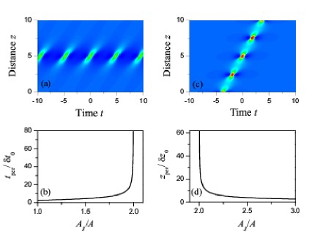
Figure 3: (Color online) (a) and (c) The evolution plots of the solutions (5) and (7), respectively, where the parameters are the same as in Fig. 1 except for $A_{s}=1.5A$ in (a) and $A_{s}=2.5A$ in (c); (b) and (d) the dependences of the ratio $t_{\text{per}}/\delta t_{0}$ and $z_{\text{per}}/\delta z_{0}$ on $A_{s}/A$, respectively.

When $A_{s}^{2}>4A^{2}$, the solution (3) can reduce to the following form

$$q(z,t)=\left(\Omega_{I}\frac{\Omega_{I}\cos\varphi+iA_{s}\sin\varphi}{A_{s}\cosh\theta-2A\cos\varphi}-A\right)e^{i\varphi_{c}},$$ (7)

where $\theta=\mu\Omega_{I}T-\mu\Omega_{I}[2\omega\alpha_{1}+(3\omega^{2}-2\mu^{2}A^{2}-\mu^{2}A_{s}^{2})\alpha_{3}]Z$ and $\varphi=\mu^{2}A_{s}\Omega_{I}(\alpha_{1}+3\omega\alpha_{3})Z$ with $\Omega_{I}=\sqrt{A_{s}^{2}-4A^{2}}$. Here $K_{\theta}=1/[2\omega\alpha_{1}+(3\omega^{2}-2\mu^{2}A^{2}-\mu^{2}A_{s}^{2})\alpha_{3}]$ and $K_{\varphi}=0$. Especially since $A_{s}\gg 2A$, namely $\Omega_{I}\sim A_{s}$, the solution (7) can be approximated as $q(z,t)\approx q_{s}(z,t)-q_{c}(z,t)$, which is the superposition of a CW solution and a bright soliton with the larger amplitude $A_{s}$. From the solution (7), one can see that it is a periodic function with period $z_{\text{per}}=2\pi/\mu^{2}A_{s}\Omega_{I}(\alpha_{1}+3\omega\alpha_{3})$ along the $z$ axis and is localized along the $t$ axis, possessing the periodic peaking property of the field amplitude like the Kuznetsov-Ma soliton (KMS) Kuznetsov ; Ma ; Xu , and so is usually called Kuznetsov-Ma soliton, as shown in Fig. 3(c). In this case, the solution (7) can reduce to the bright soliton $q_{s}(z,t)$ as $A\rightarrow 0$, and with the increasing of $A$, the bright soliton is periodized due to the interaction with the CW background and forms a KMS, and eventually reduces into the PS. This process represents the reduction of bright soliton$\rightarrow$KMS$\rightarrow$PS. Similarly, this process can be described by the ratio between the period $z_{\text{per}}=2\pi/\mu^{2}A_{s}\Omega_{I}(\alpha_{1}+3\omega\alpha_{3})$ and $\delta z_{0}$ in the form

$$\frac{z_{\text{per}}}{\delta z_{0}}=\frac{\pi}{\cos^{-1}\left[\frac{A_{s}(-7A^{2}-2AA_{s}+A_{s}^{2})}{2A(A^{2}-2AA_{s}-A_{s}^{2})}\right]},$$ (8)

where $\delta z_{0}$ is defined as the distance between two corresponding locations of half of the peak intensity along the slope direction $K_{\theta}$. Figure 3(d) presents the dependence of the ratio $z_{\text{per}}/\delta z_{0}$ on $A_{s}/A$. From it, one can see that when $A_{s}/A$ approaches $2$, the ratio $z_{\text{per}}/\delta z_{0}$ tends to infinity, which means that the distance between peaks is more and more large, eventually resulting in the formation of the PS. Similarly, the expression (8) does not depend on the parameter $\alpha_{3}$.

Another feature of PS can be described by the $z$-independent integral and the energy exchange between the PS and the CW background. Indeed, by introducing the light intensity against the CW background as follows,

$$E_{c}(t,z) =\left|q_{p}\left(t,z\right)\right|^{2}-\left|q_{p}\left(\pm\infty,z\right)\right|^{2}$$

$$=A^{2}\frac{8+32C^{2}Z^{2}-32B^{2}\left(T-DZ\right)^{2}}{[1+4C^{2}Z^{2}+4B^{2}\left(T-DZ\right)^{2}]^{2}},$$ (9)

it can be shown that it possesses the $z$-independent integral property, i. e. $\int_{-\infty}^{+\infty}E_{c}(t,z)dt=0$. From the condition $E_{c}(t_{0}\pm 1/2B,z_{0})=0$, one can define the width of PS as $1/B$, and have integrals $\int_{-1/2B}^{+1/2B}E_{c}(t,z_{0})dt=4A^{2}/B$ and $\int_{-\infty}^{-1/2B}E_{c}(t,z_{0})dt+\int_{+1/2B}^{\infty}E_{c}(t,z_{0})dt=-4A^{2}/B$. These results show that the energy of PS with stronger intensity mainly concentrates in its central interval $(-1/2B,1/2B)$, but as a result of $z$-independent integral properties, it loses the same energy in the background so that the relation $S_{1}+S_{2}=S_{3}$ holds, as shown in Figs. 4(a)-4(c). It should be noted that because $B=\mu A$ is independent of the higher-order terms in Eq. (2), the higher-order effects do not influence this property on the PS.

The energy exchange between the PS and the CW background is of the form

$$E_{e}(z) =\int_{-\infty}^{+\infty}\left|q_{p}\left(t,z\right)-q_{p}\left(\pm\infty,z\right)\right|^{2}dt$$

$$=\frac{4A^{2}\pi}{B\sqrt{1+4[2B^{2}(\alpha_{1}+3\omega\alpha_{3})]^{2}Z^{2}}}.$$ (10)

From the expression (10), one can see that $E_{e}(z)$ is a periodic function of $z$, which differs from the periodic exchange between the bright soliton and the CW background in Eq. (3) lishuqing . Also, one finds that $E_{e}(z)$ is monotonously increasing as $z<z_{0}$ and is monotonously decreasing as $z>z_{0}$; thus it takes a maximal value at $z=z_{0}$, as shown in Fig. 4(d). This result shows that at $z=z_{0}$ the energy exchange between the PS and the CW background reaches maximum. In order to understand the influence of the higher-order effects on the PS, Fig. 4(d) presents the evolution plots of $E_{e}(z)$ for different TOD parameter $\alpha_{3}$. From it, one can see that the increase of the TOD parameters $\alpha_{3}$ can enhance the rate of the energy exchange, as shown in Figs. 4(a) and 4(b).

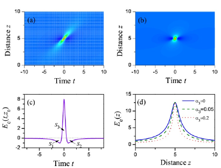
Figure 4: (Color online) The evolution plots of the Peregrine solution given by Eq. (4) for $\alpha_{3}=0$ in (a) and $\alpha_{3}=0.2$ in (b), respectively. (c) The distribution of the light intensity against the CW background given by Eq. (9) at $z=z_{0}$. (d) The evolutions of the energy exchange between the PS and the CW background for the different TOD parameters. Here the parameters are $A=1$, $\omega=1$, $t_{0}=0$, $z_{0}=5$, $\mu=1$, and $\alpha_{1}=0.5$.

III Initial excitations of the Peregrine rogue waves

In this section we will discuss the initial excitations of the Peregrine rogue wave. We start with considering the excitation of the Peregrine rogue wave based on the solutions (5) and (7). For solution (5), by linearizing its initial expression, one finds that the initial expression of the solution (5) can be approximated by

$$q_{\pm}(0,t)\approx\left(\rho_{\pm}+\epsilon_{\pm}\cos\varphi\right)e^{i\varphi_{c}(0,t)},$$ (11)

where $\rho_{\pm}=(2A^{2}-A_{s}^{2}\mp iA_{s}\Omega_{R})/(2A)$ with $\left|\rho_{\pm}\right|=A$, $\epsilon_{\pm}=A_{s}\Omega_{R}(\Omega_{R}\mp iA_{s})/(2A^{2})\exp[\mp\mu^{2}A_{s}(\alpha_{1}+3\omega\alpha_{3})\Omega_{R}z_{0}]$, and $\varphi=\mu\Omega_{R}T+\mu\Omega_{R}[2\omega\alpha_{1}+(3\omega^{2}-2\mu^{2}A^{2}-\mu^{2}A_{s}^{2})\alpha_{3}]z_{0}$. Here the subscripts “$+$” and “$-$” correspond to the case of $\alpha_{1}+3\omega\alpha_{3}>0$ and $\alpha_{1}+3\omega\alpha_{3}<0$, respectively. It can be shown that $\epsilon_{\pm}\rightarrow 0$ as $A_{s}\rightarrow 2A$. Thus the expression (11) can be regarded as an initial condition with a small periodic perturbation of background with the period $t_{\text{per}}$. The numerical simulations show that the evolution of the exact solution (5) can be well described by the initial approximation (11) (also see Ref. lishuqing ). Here one makes use of the initial approximation (11) to excite the Peregrine rogue wave as $A_{s}$ closes to $2A$.

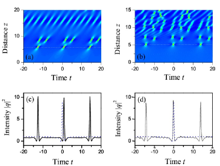
Figure 5: (Color online) The evolution plots of the numerical solution of Eq. (2) with the initial condition (11) and the comparisons of the intensity profiles of numerical and exact results at peak position, respectively: (a,c) $\alpha_{3}=0$, (b,d) $\alpha_{3}=0.2$. Note that in (c) and (d), the blue dotted curves are the exact results given by Eq. (4) at $z=z_{0}$ and the black solid curves are the numerical results at $z=5.9$ in (a) and $z=5.2$ in (b) [the white dotted lines in (a) and (b)], respectively. Here $A_{s}=1.95$, and other parameters are the same as in Fig. 4.

Figure 5 presents the evolution plots of the numerical solution of Eq. (2) with the initial condition (11) and the comparisons of the intensity profile between numerical and exact Peregrine rogue waves at peak position for $\alpha_{3}=0$ and $\alpha_{3}\neq 0$, respectively. From it, one can see that when $A_{s}$ approaches to $2A$, the initial condition (11) evolves into a string of near-ideal Peregrine rogue waves. Although the theoretical results reveal that there is a Peregrine rogue wave only in the limitation of $A_{s}\rightarrow 2A$, in practice, this cannot be implemented due to $\epsilon_{\pm}=0$ as $A_{s}=2A$. Furthermore, from Figs. 5(a) and 5(b), it can be seen that the evolution for long distances shows the breakup of the Peregrine rogue wave, which implies that the Peregrine rogue wave is unstable. Also, from Figs. 5(c) and 5(d), one can see that the presence of the higher-order effects did not markedly influence the intensity distribution of the Peregrine rogue wave at peak position, except for a displacement of the peak position, but shortens the distance of energy exchange, as shown in Figs. 5(a) and 5(b). This is in agreement with that suggested in Fig. 4(d).

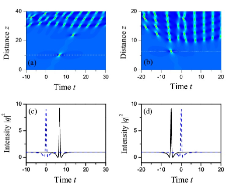
Figure 6: (Color online) The evolution plots of the numerical solution of Eq. (2) with the initial condition (12) and the comparisons of the corresponding intensity profile at peak position, respectively: (a,c) $\alpha_{3}=0$, (b) and (d) $\alpha_{3}=0.2$. Note that in (c,d), the blue dotted curves are the exact results given by Eq. (4) at $z=z_{0}$ and the black solid curves are the numerical results at $z=10.2$ in (a) and $z=6.4$ in (b) [the white dotted lines in (a) and (b)], respectively. Here $A_{s}=2.05$, $\omega=0.5$, and other parameters are the same as in Fig. 4.

In the following, we discuss the initial excitation induced by the solution (7). In this case, one find that the solution (7) can take the following particular form

$$q(z_{1},t) =\left(-A+i\Omega_{I}\operatorname{sech}\theta\right)e^{i\varphi_{c}(z_{1},t)}$$

$$=Ae^{i\left[\varphi_{c}(z_{1},t)+\pi\right]}+\Omega_{I}\operatorname{sech}\theta e^{i\left[\varphi_{c}(z_{1},t)+\frac{\pi}{2}\right]}$$ (12)

at the location $z_{1}=(2n\pi+\pi/2)/[\mu^{2}A_{s}\Omega_{I}(\alpha_{1}+3\omega\alpha_{3})]+z_{0}$, $n=0,\pm 1,\pm 2,\cdots$, where $\theta=\mu\Omega_{I}T-[2\omega\alpha_{1}+(3\omega^{2}-2\mu^{2}A^{2}-\mu^{2}A_{s}^{2})\alpha_{3}](2n\pi+\pi/2)/[\mu A_{s}(\alpha_{1}+3\omega\alpha_{3})]$. Without loss of generality, here we take $n=0$. The expression (12) is the superposition of a CW and an aperiodic hyperbolic secant function, especially as $A_{s}\rightarrow 2A$, $\Omega_{I}$ tends to zero. This means that the expression (12) can be regarded as an initial condition with a small aperiodic (simple peak) perturbation of background, which differs from the superposition of a CW and a periodic perturbation in the expression (11). Here we make use of the expression (12) as an initial condition to investigate the excitation of the Peregrine rogue wave. Similarly, the numerical simulations show that the evolution of the exact solution (7) can be well described by the initial condition (12) except for a translation.

Figure 6 shows the evolutions of the numerical solution of Eq. (2) with the initial condition (12) and the comparisons of the intensity profile of numerical and exact Peregrine rogue waves at peak position for $\alpha_{3}=0$ and $\alpha_{3}\neq 0$, respectively. From it, one can see that the initial condition (12) evolves into a near-ideal Peregrine rogue wave, which differs from that shown in Figs. 5(a) and 5(b). Similarly, Figs. 6(a) and 6(b) show the breakup of the Peregrine rogue wave for long distance, which implies that the Peregrine rogue wave is unstable.

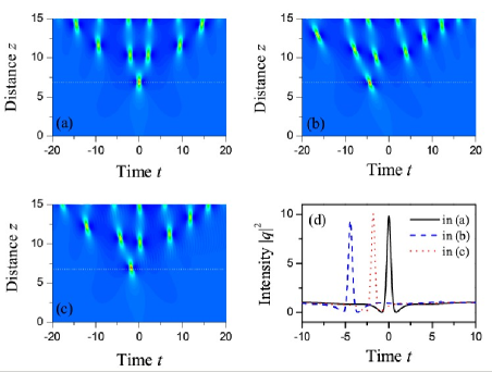
Figure 7: (Color online) The numerical evolution plots of the initial condition (13): (a) for NLS equation with $\alpha_{3}=0;$ (b) for Hirota equation (2) with $\alpha_{3}=0.1;$ (c) for HNLS equation (1) with $\alpha_{3}=0.05$, $\alpha_{4}=0.285,$ and $\alpha_{5}=-0.315;$ and (d) the distributions of the intensity profile at $z=6.975$ in (a), $z=6.825$ in (b), and $z=6.9$ in (c). Here $\alpha_{1}=0.5$, $A=1$, $\epsilon=0.05,$ and $\sigma=0.05$.

Comparing results in Figs. 5 and 6, we find that a small localized (single-peak) perturbation pulse of CW background can excite a Peregrine rogue wave. Indeed, every peak in the initial expression (11) can excite a Peregrine rogue wave; thus a periodic perturbation of background resulted in the generation of a string of the Peregrine rogue waves, as shown in Figs. 5(a) and 5(b). So we can suggest that the Peregrine rogue wave can be excited by the interaction between the CW and a small localized (single-peak) perturbation pulse. As an example, we consider a simple initial condition with a Gaussian-type perturbation pulse as follows

$$q(0,t)=A+\epsilon\exp(-\sigma t^{2}),$$ (13)

where $\epsilon$ is a modulation amplitude and a small quantity. The numerical simulations show that when the width of the initial perturbation pulse is wide enough, i. e, the parameter $\sigma$ is small enough, the Peregrine rogue wave can be excited by the initial condition (13) even for a nonintegrable HNLS equation (1). Figure 7 shows the evolution plots of the numerical solution for Eq. (1) with the initial condition (13), which includes a numerical evolution of the initial condition (13) under the nonintegrable case, as shown in Fig. 7(c). From Fig. 7(d), one can see that the main characteristics of the Peregrine rogue wave are maintained. Certainly, the Peregrine rogue wave is unstable. This result can be used to understand extreme localized events in ocean.

IV The influence of the self-frequency shift to the dynamics of the Peregrine rogue wave

It should be noted that the equation (1) does not include the self-frequency shift effect arising from stimulated Raman scattering because the parameter $\alpha_{5}$ is a real number. In this section we discuss the influence of the self-frequency shift effect on the dynamics of the Peregrine rogue wave. In this case, the model governing pulse propagation can be written as Agrawal

$$\frac{\partial Q}{\partial\xi} =-i\frac{\beta_{{}^{2}}}{2}\frac{\partial^{2}Q}{\partial\tau^{2}}+i\gamma|Q|^{2}Q+\frac{\beta_{{}^{{}_{3}}}}{6}\frac{\partial^{3}Q}{\partial\tau^{3}}$$

$$-\frac{\gamma}{\omega_{0}}\frac{\partial|Q|^{2}Q}{\partial\tau}-i\gamma T_{R}Q\frac{\partial|Q|^{2}}{\partial\tau},$$ (14)

where $\tau$ and $\xi$ represent the temporal coordinate and the propagation distance, $\beta_{{}^{2}}$ is the group velocity dispersion, $\beta_{3}$ is the third-order dispersion, $\gamma$ is the nonlinear coefficient of the fiber, and $T_{R}$ is the Raman time constant. By introducing the dimensionless transformations $Q(\xi,\tau)=\sqrt{P_{0}}q(z,t)$, $t=\tau/T_{0}$, and $z=\xi/L_{D}$ with the dispersion length $L_{D}=T_{0}^{2}/|\beta_{{}^{2}}|$, Eq. (14) becomes the form of Eq. (1) with the coefficients $\alpha_{1}=-\beta_{{}^{2}}/(2\left|\beta_{{}^{2}}\right|)$, $\alpha_{2}=\gamma L_{D}P_{0}$, $\alpha_{3}=\beta_{{}^{{}_{3}}}L_{D}/(6T_{0}^{3})$, $\alpha_{4}=-\gamma L_{D}P_{0}/(\omega_{0}T_{0}),$ and $\alpha_{5}=-i\gamma T_{R}L_{D}P_{0}/T_{0}$, respectively. It should be pointed out that here $\alpha_{5}$ is a complex number which describes the self-frequency shift effect arising from stimulated Raman scattering.

As an example, here we use realistic parameters for a highly nonlinear fiber at $1550$nm with the group velocity dispersion $\beta_{{}^{2}}$ $=-8.85\times 10^{-1}$ ps²/km, the third-order dispersion $\beta_{{}^{{}_{3}}}=1.331\times 10^{-2}$ ps³/km, and the nonlinear parameter $\gamma=10$ W${}^{-1}\cdot$km^-1 NatPhys . Thus, for a given initial power $P_{0}$, the parameters $\alpha_{1}$, $\alpha_{2}$, $\alpha_{3}$, $\alpha_{4}$ and $\alpha_{5}$ can be determined. Note that in our simulations we take $\alpha_{2}=1$ by choosing a temporal scale $T_{0}=[|\beta_{{}^{2}}|/(\gamma P_{0})]^{1/2}$, and the Raman time constant $T_{R}=5$fs when the self-frequency shift is considered. We still take Eq. (13) as the initial condition, in which the realistic width of the initial perturbation pulse is $T_{1}\equiv T_{0}/\sqrt{2\sigma}$.

Figure 8 presents the numerical evolution plots of the initial condition (13) with the initial perturbation pulse width $T_{1}=2$ps for the different initial power $P_{0}$. From Fig. 8 it can be seen that, in the absence of the self-frequency shift effect ($T_{R}=0$), the Peregrine rogue wave in turn splits into two subpulses, three subpulses, and so on, and can split into more subpulses for higher initial power, as shown in Figs. 8(a) and 8(b). These results are similar to the pulse splitting induced by higher-order modulation instability based on NLS equation in Ref. Erkintalo , but here the complex splitting dynamic evolutions are excited by a linear superposition of the CW and a small localized (single peak) perturbation pulse, and the higher-order effects, such as the third-order dispersion and the self-steepening, are included. However, when the self-frequency shift effect is considered, such splitting of the Peregrine rogue wave no longer appears, as shown in Figs. 8(c) and 8(d). It is surprising that, in this case, the dynamics of the Peregrine rogue wave mainly exhibit a peak changing propagation characteristic of the field amplitude except for some of the small radiations, and has an increase in peaking value, as shown in Figs. 8(e) and 8(f). This property can be used for generation of the higher peak power pulse.

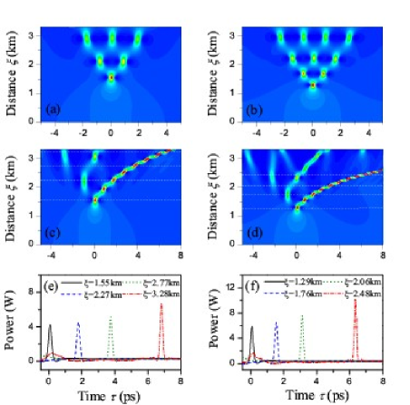
Figure 8: (Color online) The numerical evolution plots of the initial condition (13) for the different initial power: (a,b) the absence of self-frequency shift ($T_{R}=0$), (c,d) the presence of self-frequency shift ($T_{R}=5$ fs), and (e,f) the corresponding power density distributions at the different distance labeled by the white dotted lines in (c) and (d), respectively. In (a), (c), and (e), the initial power $P_{0}=0.3$W, and in (b), (d), and (f), the initial power $P_{0}=0.4$W. Here $\epsilon=0.2$ and $A=1$.

Furthermore, the dependences of the peak position $\xi_{\text{peak}}$ of the excited Peregrine rogue wave on the modulation amplitude $\epsilon$ are considered, as shown in Fig. 9. From it one can see that for a given initial perturbation pulse width $T_{1}$ or initial power $P_{0}$, the peak position $\xi_{\text{peak}}$ of the excited Peregrine rogue wave is a decreasing function of the modulation amplitude $\epsilon$. Thus one can control the position of the excited Peregrine rogue wave by suitably choosing the initial perturbation pulse width or the initial power. Also, we find that the self-frequency shift effect does not influence the peak position $\xi_{\text{peak}}$ of the excited Peregrine rogue wave.

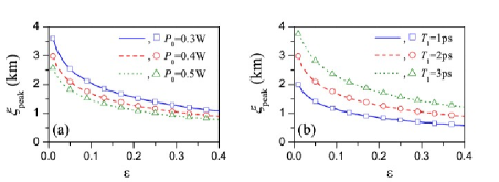
Figure 9: (Color online) The dependences of the peak position $\xi_{\text{peak}}$ of the excited Peregrine rogue wave on the modulation amplitude $\epsilon$ for (a) the different initial power and a given initial perturbation pulse width $T_{1}=2$ps, and (b) the different initial perturbation pulse width $T_{1}$ and a given initial power $P_{0}=0.4$W. Here the solid, dashed and dotted curves correspond to the results of $T_{R}=0$, and the open diamonds, circles and triangles correpond to the results of $T_{R}=5$fs, and the parameter $A=1$.

V Conclusions

In summary, based on the soliton solution on a CW background for an integrable Hirota equation, we have presented the reduction mechanism and the main characteristics of the Peregrine rogue wave in the propagation of femtosecond pulses of optical fiber. The results have shown that there exist two processes of the formation of the Peregrine rogue wave: one is the reduction of CW$\rightarrow$AB$\rightarrow$PS, which is the localized process of the CW background, and the other is the reduction of bright soliton$\rightarrow$KMS$\rightarrow$PS, which is the reduction process of the periodization of the bright soliton. The characteristics of the Peregrine rogue wave have been exhibited by strong temporal and spatial localization. Also, the initial excitations of the Peregrine rogue wave have been discussed. The results have shown that a Peregrine rogue wave can be excited by a small localized (single peak) perturbation pulse of CW background, even for the nonintegrable HNLS equation. This means that the Peregrine rogue wave is a result of interaction between the continuous wave background and soliton. Furthermore, the numerical simulations have shown that the Peregrine rogue wave is unstable. Finally, through the study for a realistic highly nonlinear fiber, it has been found that the self-frequency shift influences the dynamics of the Peregrine rogue wave. The results show that in the absence of the self-frequency shift, the Peregrine rogue wave can splits into several subpulses; however, when the self-frequency shift is considered, the Peregrine rogue wave no longer splits and exhibits mainly a peak changing and increasing propagation property.

This research was supported by the National Natural Science Foundation of China under Grant No.61078079 and the Shanxi Scholarship Council of China under Grant No.2011-010.

References

- (1) C. Kharif, E. Pelinovsky, and A. Slunyaev, Rogue Waves in the Ocean (Springer, Heidelberg, 2009).
- (2) C. Kharif and E. Pelinovsky, Eur. J. Mech. BFluids 22, 603 (2003).
- (3) A. Slunyaev, Eur. J. Mech. BFluids 25, 621 (2006).
- (4) V. E. Zakharov, A. I. Dyachenko, and A. O. Prokofiev, Eur. J. Mech. BFluids 25, 677 (2006).
- (5) V. P. Ruban, Phys. Rev. Lett. 99, 044502 (2007).
- (6) Andonowati, N. Karjanto, and E. van Groesen, App. Math. Mod 31, 1425 (2007).
- (7) D. R. Solli, C. Ropers, P. Koonath, and B. Jalali, Nature (London)(London)450, 1054 (2007).
- (8) A. N. Ganshin, V. B. Efimov, G.V. Kolmakov, L. P. Mezhov-Deglin, and P.V. E. McClintock, Phys. Rev. Lett. 101, 065303 (2008).
- (9) M. Shats, H. Punzmann, and H. Xia, Phys. Rev. Lett. 104, 104503 (2010).
- (10) J. Dudley, G. Genty, and B. Eggelton, Opt. Express 16, 3644 (2008).
- (11) D. R. Solli, C. Ropers, and B. Jalali, Phys. Rev. Lett. 101, 233902 (2008).
- (12) A. Mussot, A. Kudlinski, M. Kolobov, E. Louvergneaux, M. Douay and M. Taki, Opt. Express 17, 17010 (2010).
- (13) M. Taki, A. Mussot, A. Kudlinski, E. Louvergneaux, M. Kolobov, and M. Douay, Phys. Lett. A 374, 691 (2010).
- (14) A. R. Osborne, M. Onorato, and M. Serio, Phys. Lett. A 275, 386 (2000).
- (15) A. R. Osborne, Mar. Struct. 14, 275 (2001).
- (16) N. Akhmediev, A. Ankiewicz, and M. Taki, Phys. Lett. A 373, 675 (2009).
- (17) N. Akhmediev, J. M.Soto-Crespo, and A. Ankiewicz, Phys. Lett. A 373, 2137 (2009).
- (18) A. Ankiewicz, N. Devine, and N. Akhmediev, Phys. Lett. A 373, 3997 (2009).
- (19) N. Akhmediev, J. M. Soto-Crespo, and A. Ankiewicz, Phys. Rev. A80, 043818 (2009).
- (20) N. Akhmediev, A. Ankiewicz, and J. M. Soto-Crespo, Phys. Rev. E80, 026601 (2009).
- (21) Zhenya Yan, Phys. Lett. A 374, 672 (2010).
- (22) M. Erkintalo, K. Hammani, B. Kibler, Ch. Finot, N. Akhmediev, J. M. Dudley, and G. Genty, Phys. Rev. Lett. 107, 253901 (2011).
- (23) B. Kibler, K. Hammani, C. Michel, Ch. Finot, and A. Picozzi, Phys. Lett. A 375, 3149 (2011).
- (24) D. H. Peregrine, J. Austral. Math. Soc. Ser. B25, 16 (1983).
- (25) E. A. Kuznetsov, Sov. Phys. Dokl. 22, 507 (1977).
- (26) Ya. C. Ma, Stud. Appl. Math. 60, 43 (1979).
- (27) N. Akhmediev and V. I. Korneev, Theor. Math. Phys. 69, 1089 (1986).
- (28) B. Kibler, J. Fatome, C. Finot, G. Millot, F. Dias, G. Genty, N. Akhmediev, and J. M. Dudley, Nat. Phys. 6, 790 (2010).
- (29) K. Hammani, B. Kibler, C. Finot, Ph. Morin, J. Fatome, J. M. Dudley, and G. Millot, Opt. Lett. 36, 112 (2011).
- (30) Y. Kodama and A. Hasegawa, IEEE J. Quantum Electron. 23, 510 (1987).
- (31) R. Hirota, J. Math. Phys. 14, 805 (1973) .
- (32) M. Lakshmanan and S. Ganesan, J. Phys. Soc. Jpn. 52, 4031 (1983).
- (33) D. Mihalache, L. Torner, F. Moldoveanu, N.-C. Panoiu, and N. Truta, Phys. Rev. E48, 4699 (1993).
- (34) D. Mihalache, N.-C. Panoiu, F. Moldoveanu, and D.-M. Baboiu, J. Phys. A: Math. Gen. 27, 6177 (1994).
- (35) K. Porsezian and K. Nakkeeran, Phys. Rev. Lett. 76, 3955 (1996).
- (36) D. Mihalache, N. Truta, and L. C. Crasovan, Phys. Rev. E56, 1064 (1997).
- (37) L. Li, Z. H. Li, Z. Y. Xu, G. S. Zhou, and K. H. Spatscheck, Phys. Rev. E66, 046616 (2002).
- (38) Z. Y. Xu, L. Li, Z. H. Li, and G. S. Zhou, Phys. Rev. E67, 026603 (2003).
- (39) S. Q. Li, L. Li, Z. H. Li, and G. S. Zhou, J. Opt. Soc. Am. B21, 2089 (2004).
- (40) A. Ankiewicz, J. M. Soto-Crespo, and N. Akhmediev, Phys. Rev. E81, 046602 (2010).
- (41) Q. H. Park and H. J. Shin, Phys. Rev. Lett. 82, 4432 (1999).
- (42) M. J. Ablowitz, and P. A. Clarkson, Soliton, Nonlinear Evolution Equations and Inverse Scattering (University Press, Cambridge, 1991).
- (43) G. P. Agrawal, Nonlinear Fiber Optics (Academic Press, New York, 1995).