Adaptive parallel tempering algorithm

Abstract.

Parallel tempering is a generic Markov chain Monte Carlo sampling method which allows good mixing with multimodal target distributions, where conventional Metropolis-Hastings algorithms often fail. The mixing properties of the sampler depend strongly on the choice of tuning parameters, such as the temperature schedule and the proposal distribution used for local exploration. We propose an adaptive algorithm which tunes both the temperature schedule and the parameters of the random-walk Metropolis kernel automatically. We prove the convergence of the adaptation and a strong law of large numbers for the algorithm. We illustrate the performance of our method with examples. Our empirical findings indicate that the algorithm can cope well with different kind of scenarios without prior tuning.

1. Introduction

Markov chain Monte Carlo (MCMC) is a generic method to approximate an integral of the form

$$I\stackrel{{\scriptstyle\mathrm{def}}}{{=}}\int_{\mathbb{R}^{d}}f(x)\pi(x)\mathrm{d}x\,,$$

where $\pi$ is a probability density function, which can be evaluated point-wise up to a normalising constant. Such an integral occurs frequently when computing Bayesian posterior expectations [e.g., 24, 11].

The random-walk Metropolis algorithm [21] works often well, provided the target density $\pi$ is, roughly speaking, sufficiently close to unimodal. The efficiency of the Metropolis algorithm can be optimised by a suitable choice of the proposal distribution. The proposal distribution can be chosen automatically by several adaptive MCMC algorithms; see [12, 4, 26, 2] and references therein.

When $\pi$ has multiple well-separated modes, the random-walk based methods tend to get stuck to a single mode for long periods of time, which can lead to false convergence and severely erroneous results. Using a tailored Metropolis-Hastings algorithm can help, but in many cases finding a good proposal distribution is difficult. Tempering of $\pi$, that is, considering auxiliary distributions with density proportional to $\pi^{\beta}$ with $\beta\in(0,1)$ often provides better mixing within modes [30, 20, 13, 34]. We focus here particularly on the parallel tempering algorithm, which is also known as the replica exchange Monte Carlo and the Metropolis coupled Markov chain Monte Carlo.

The tempering approach is particularly tempting in such settings where $\pi$ admits a physical interpretation, and there is good intuition how to choose the temperature schedule for the algorithm. In general, choosing the temperature schedule is a non-trivial task, but there are generic guidelines for temperature selection, based on both empirical findings and theoretical analysis. First rule of thumb suggests that the temperature progression should be (approximately) geometric; see, e.g. [16]. Kone and Kofke linked also the mean acceptance rate of the swaps [17]; this has been further analysed by Atchadé, Roberts and Rosenthal [5]; see also [27].

Our temperature adaptation is based on the latter; we try to optimise the mean acceptance rate of the swaps between the chains in adjacent temperatures. Our scheme has similarities with that proposed by Atchadé, Roberts and Rosenthal [5]. The key difference in our method is that we propose to adapt continuously during the simulation. We show that the temperature adaptation converges, and that the point of convergence is unique with mild and natural conditions on the target distribution.

The local exploration in our approach relies on the random walk Metropolis algorithm. The proposal distribution, or more precisely, the scale/shape parameter of the proposal distribution, can be adapted using several existing techniques like the covariance estimator [12] augmented with an adaptive scaling pursuing a given mean acceptance rate [2, 3, 26, 4] which is motivated by certain asymptotic results [25, 28]. It is also possible to use a robust shape estimate which enforces a given mean acceptance rate [33].

We start by describing the proposed algorithm in Section 2. Theoretical results on the convergence of the adaptation and the ergodic averages are given next in Section 3. In Section 4, we illustrate the performance of the algorithm with examples. The proofs of the theoretical results are postponed to Section 5.

2. Algorithm

2.1. Parallel tempering algorithm

The parallel tempering algorithm defines a Markov chain over the product space $\mathsf{X}^{L}$, where $\mathsf{X}\subset\mathbb{R}^{d}$

(1) $$\mathbf{X}_{k}=(X_{k}^{(1)},\ldots,X_{k}^{(L)})=(X_{k}^{(1:L)})\,.$$

Each of the chains $X_{k}^{(\ell)}$ targets a ‘tempered’ version of the target distribution $\pi$. Denote by $\boldsymbol{\beta}=(\beta^{(1:L)})$ the inverse temperature, which are such that $1=\beta^{(1)}>\beta^{(2)}>\cdots>\beta^{(L)}>0$. and by $Z(\beta)$ the normalising constant

(2) $$Z(\beta)\stackrel{{\scriptstyle\mathrm{def}}}{{=}}\int\pi^{\beta}(x)\mathrm{d}x\,,$$

which is assumed to be finite. The parallel tempering algorithm is constructed so that the Markov chain $\{\mathbf{X}_{k}\}_{k\geq 0}$ is reversible with respect to the product density

(3) $$\boldsymbol{\pi}_{\boldsymbol{\beta}}(x^{(1)},\ldots,x^{(L)})\stackrel{{\scriptstyle\mathrm{def}}}{{=}}\frac{\pi^{\beta^{(1)}}(x^{(1)})}{Z(\beta^{(1)})}\times\cdots\times\frac{\pi^{\beta^{(L)}}(x^{(L)})}{{Z(\beta^{(L)})}}\,,$$

over the product space $(\mathsf{X}^{L},\mathcal{X}^{\otimes L})$.

Each time-step may be decomposed into two successive moves: the swap move and the propagation (or update) move; for the latter, we consider only random-walk Metropolis moves.

We use the following notation to distinguish the state of the algorithm after the swap step (denoted $\bar{\mathbf{X}}_{n}$) and after the random walk step, or equivalently after a complete step (denoted $\mathbf{X}_{n}$). The state is then updated according to

(4) $$\mathbf{X}_{n-1}\stackrel{{\scriptstyle\mathbf{S}_{\boldsymbol{\beta}}}}{{\longrightarrow}}\bar{\mathbf{X}}_{n-1}\stackrel{{\scriptstyle\mathbf{M}_{(\boldsymbol{\Sigma},\boldsymbol{\beta})}}}{{\longrightarrow}}\mathbf{X}_{n},$$

where the two kernels $\mathbf{M}_{(\boldsymbol{\Sigma},\boldsymbol{\beta})}$ and $\mathbf{S}_{\boldsymbol{\beta}}$ are respectively defined as

• $\mathbf{M}_{(\boldsymbol{\Sigma},\boldsymbol{\beta})}$ denotes the tensor product kernel on the product space $\mathsf{X}^{L}$

  (5) $$\mathbf{M}_{(\boldsymbol{\Sigma},\boldsymbol{\beta})}(x^{(1:L)};A_{1}\times\dots A_{L})=\prod_{\ell=1}^{L}M_{(\Sigma^{(\ell)},\beta^{(\ell)})}(x^{(\ell)},A_{\ell})$$

  where each $M_{(\Sigma^{(\ell)},\beta^{(\ell)})}$ is a random-walk Metropolis kernel targeting $\pi^{\beta^{(\ell)}}$ with increment distribution $q_{\Sigma^{(\ell)}}$, where $q_{\Sigma}$ is the density of a multivariate Gaussian with zero mean and covariance $\Sigma$,

  (6) $$M_{(\Sigma,\beta)}(x,A)\stackrel{{\scriptstyle\mathrm{def}}}{{=}}\int_{A}\alpha_{\beta}(x,y)q_{\Sigma}(y-x)\mathrm{d}y\\ +\delta_{x}(A)\int(1-\alpha_{\beta}(x,y))q_{\Sigma}(y-x)\mathrm{d}y\,,$$

  where

  (7) $$\alpha_{\beta}(x,y)\stackrel{{\scriptstyle\mathrm{def}}}{{=}}1\wedge\frac{\pi^{\beta}(y)}{\pi^{\beta}(x)}\,,\quad\text{for all $(x,y)\in\mathsf{X}\times\mathsf{X}$}\,.$$

  In practical terms, $\mathbf{M}_{(\boldsymbol{\Sigma},\boldsymbol{\beta})}$ means that one applies a random-walk Metropolis step separately for each of the chains $\bar{X}_{n-1}^{(\ell)}$.

• $\mathbf{S}_{\boldsymbol{\beta}}$ denotes the Markov kernel of the swap steps, targeting the product distribution $\boldsymbol{\pi}_{\boldsymbol{\beta}}\propto\pi^{\beta^{(1)}}\otimes\cdots\otimes\pi^{\beta^{(L)}}$,

  (8) $$\mathbf{S}_{\boldsymbol{\beta}}(x^{(1:L)};A)=\frac{1}{L-1}\sum_{j=1}^{L-1}\varpi^{(j)}_{\boldsymbol{\beta}}(x^{(j)},x^{(j+1)})J^{(j)}(x^{(j)},x^{(j+1)};A)\\ +\frac{1}{L-1}\sum_{j=1}^{L-1}(1-\varpi^{(j)}_{\boldsymbol{\beta}}(x^{(j)},x^{(j+1)}))\;\delta_{x^{(1:L)}}(A)\,,$$

  where $\varpi^{(j)}_{\boldsymbol{\beta}}$ is the probability of accepting a swap between levels $j$ and $j+1$, which is given by

  (9) $$\varpi^{(j)}_{\boldsymbol{\beta}}(x^{(j)},x^{(j+1)})\stackrel{{\scriptstyle\mathrm{def}}}{{=}}1\wedge\left(\frac{\pi(x^{(j+1)})}{\pi(x^{(j)})}\right)^{\beta^{(j)}-\beta^{(j+1)}}\,,$$

  and

  (10) $$J^{(j)}(x^{(j)},x^{(j+1)};A)\\ \stackrel{{\scriptstyle\mathrm{def}}}{{=}}\idotsint_{A}\delta_{x^{(j)}}(\mathrm{d}y^{(j+1)})\delta_{x^{(j+1)}}(\mathrm{d}y^{(j)})\prod_{i\in\{1,\dots,L\}\setminus\{j,j+1\}}\delta_{x^{(i)}}(\mathrm{d}y^{(i)})\,.$$

  The above defined swap step means choosing a random index $\ell\in\{1,\ldots,L-1\}$ uniformly, and then proposing to swap the adjacent states, $\bar{X}_{n-1}^{(\ell+1)}=X_{n-1}^{(\ell)}$ and $\bar{X}_{n-1}^{(\ell)}=X_{n-1}^{(\ell+1)}$. and accepting this swap with probability given in (9).

2.2. Adaptive parallel tempering algorithm

In the adaptive version of the parallel tempering algorithm, the temperature parameters are continuously updated along the run of the algorithm. We denote the sequence of inverse temperatures

(11) $$\left\{\boldsymbol{\beta}_{n}\right\}_{n\geq 0}=\left\{\beta_{n}^{(1:L)}\right\}_{n\geq 0}$$

which are parameterised by the vector-valued process

(12) $$\left\{\boldsymbol{\rho}_{n}\right\}_{n\geq 0}\stackrel{{\scriptstyle\mathrm{def}}}{{=}}\left\{\rho_{n}^{(1:L-1)}\right\}_{n\geq 0}\,,$$

through $\beta_{n}^{(1)}\stackrel{{\scriptstyle\mathrm{def}}}{{=}}1$ and $\beta_{n}^{(\ell)}=\beta^{(\ell)}(\rho^{(1:\ell-1)}_{n})$ for $\ell\in\{2,\dots,L\}$ with

(13) $$\beta^{(\ell+1)}(\rho^{(1:\ell)})\stackrel{{\scriptstyle\mathrm{def}}}{{=}}\beta^{(\ell)}(\rho^{(1:\ell-1)})\exp(-\exp(\rho^{(\ell)}))\,.$$

Because the inverse temperatures are adapted at each iteration, the target distribution of the chain changes from step to step as well. Our adaptation of the temperatures is performed using the following stochastic approximation procedure

(14) $$\rho^{(\ell)}_{n}=\Pi_{\rho}\left(\rho^{(\ell)}_{n-1}+\gamma_{n,1}H^{(\ell)}(\rho_{n-1}^{(1:\ell)},\mathbf{X}_{n})\right)\,,\qquad 1\leq\ell\leq L-1\,,$$

where $(\rho_{n}^{(1:L-1)})$ is defined in (13), $\Pi_{\rho}$ is the projection onto the constraint set $\left[\underline{\rho},\overline{\rho}\right]$, which will be discussed further in Section 2.4. Moreover,

(15) $$H^{(\ell)}(\rho^{(1:\ell)},\mathbf{x})=1\wedge\left(\frac{\pi(x^{(\ell+1)})}{\pi(x^{(\ell)})}\right)^{\Delta\beta^{(\ell)}(\rho^{(1:\ell)})}-\alpha^{*}\,,$$

(16) $$\Delta\beta^{(\ell)}(\rho^{(1:\ell)})=\beta^{(\ell)}(\rho^{(1:\ell-1)})-\beta^{(\ell+1)}(\rho^{(1:\ell)})\,.$$

We will show in Section 3 that the algorithm is designed in such a way that the inverse temperatures converges to a value for which the mean probability of accepting a swap move between any adjacent-temperature chains is constant and is equal to $\alpha^{*}$.

We will also adapt the random-walk proposal distribution at each level. We describe below another possible algorithm for performing such a task. In the theoretical part, for simplicity, we will consider only on with the seminal adaptive Metropolis algorithm [12] augmented with scaling adaptation [e.g. 26, 3, 2]. In this algorithm, we estimate the covariance matrix of the target distribution at each temperature and rescale it to control the acceptance ratio at each level in stationarity.

Define by $\mathcal{M}_{+}(d)$ the set of $d\times d$ positive definite matrices. For $A\in\mathcal{M}_{+}(d)$, we denote by $\varrho_{\min}(A)$ and $\varrho_{\max}(A)$ the smallest and the largest eigenvalues of $A$, respectively. For $\varepsilon\in(0,1]$, define by $\mathcal{M}_{+}(d,\varepsilon)\subset\mathcal{M}_{+}(d)$ the convex subset

(17) $$\mathcal{M}_{+}(d,\varepsilon)\stackrel{{\scriptstyle\mathrm{def}}}{{=}}\left\{\Sigma\in\mathcal{M}_{+}(d):\varepsilon\leq\varrho_{\min}(\Sigma)\leq\varrho_{\max}(\Sigma)\leq\varepsilon^{-1}\right\}\,.$$

The set $\mathcal{M}_{+}(d,\varepsilon)$ is a compact subset of the open cone of positive definite matrices.

We denote by $\Gamma_{n}^{(\ell)}$ the current estimate of the covariance at level $\ell$, which is updated as follows

(18) $$\Gamma_{n}^{(\ell)} =\Pi_{\Gamma}\left[(1-\gamma_{n,2})\Gamma_{n-1}^{(\ell)}+\gamma_{n,2}(X_{n}^{(\ell)}-\mu_{n-1}^{(\ell)}){t(X_{n}^{(\ell)}-\mu_{n-1}^{(\ell)})}\right],$$

(19) $$\mu_{n}^{(\ell)} =(1-\gamma_{n,2})\mu_{n-1}^{(\ell)}+\gamma_{n,2}X_{n}^{(\ell)}\,,$$

where $t(\cdot)$ is the matrix transpose and $\Pi_{\Gamma}$ is the projection on to the set $\mathcal{M}_{+}(d,\varepsilon)$; see Section 2.4. The scaling parameters is updated so that the acceptance rate in stationarity converges to the target $\alpha^{\star}$,

(20) $$T_{n}^{(\ell)}=\Pi_{T}\left(T_{n-1}^{(\ell)}+\gamma_{n,3}\left[\left(1\wedge\frac{\pi^{\beta^{(\ell)}_{n-1}}(Y^{(\ell)}_{n})}{\pi^{\beta^{(\ell)}_{n-1}}(\bar{X}_{n-1}^{(\ell)})}\right)-\alpha^{*}\right]\right)\,,$$

where $\Pi_{T}$ is is the projection onto $\left[\underline{T},\overline{T}\right]$; see Section 2.4 and $Y_{n}^{(\ell)}$ is the proposal at level $\ell$, assumed to be conditionally independent from the past draws and distributed according to a Gaussian with mean $\bar{X}_{n-1}^{(\ell)}$ and covariance matrix $\Sigma^{(\ell)}_{n-1}$ which is given by

(21) $$\Sigma^{(\ell)}_{n}=\exp(T_{n}^{(\ell)})\,\Gamma_{n}^{(\ell)}\,.$$

In the sequel we denote by $\mathbf{Y}_{n}$ the vector of proposed moves at time step $n$,

(22) $$\{\mathbf{Y}_{n}\}_{n\geq 0}=\{Y_{n}^{(1:L)}\}_{n\geq 0}\,.$$

2.3. Alternate random-walk adaptation

In order to reduce the number of parameters in the adaptation especially in higher dimensions, we propose to use a common covariance for all the temperatures, but still employ separate scaling. More specifically,

(23) $$\Gamma_{n} =(1-\gamma_{n,2})\Gamma_{n-1}+\frac{\gamma_{n,2}}{L}\sum_{\ell=1}^{L}(X_{n}^{(\ell)}-\mu_{n-1})t(X_{n}^{(\ell)}-\mu_{n-1})\,,$$

(24) $$\mu_{n} =(1-\gamma_{n,2})\mu_{n-1}+\frac{\gamma_{n,2}}{L}\sum_{\ell=1}^{L}X_{n}^{(\ell)}\,,$$

and set $\Sigma_{n}^{(\ell)}=\exp(T_{n}^{(\ell)})\Gamma_{n}$.

Another possible implementation of the random-walk adaption, robust adaptive Metropolis (RAM) [33], is defined by a single dynamic adjusting the covariance parameter and attaining a given acceptance rate. Specifically, one recursively finds a lower-diagonal matrix $\Gamma_{n}^{(\ell)}\in\mathbb{R}^{d\times d}$ with positive diagonal satisfying

(25) $$\Gamma_{n}^{(\ell)}t({\Gamma}_{n}^{(\ell)})=\Gamma_{n-1}^{(\ell)}\left[I+\gamma_{n,2}(\alpha_{n}-\alpha^{*})u(Z_{n}^{(\ell)})t\big{(}u(Z_{n}^{(\ell)})\big{)}\right]t({\Gamma}_{n-1}^{(\ell)})\,,$$

where $Z_{n}^{(\ell)}\stackrel{{\scriptstyle\mathrm{def}}}{{=}}Y_{n}^{(\ell)}-\bar{X}_{n-1}^{(\ell)}$ and $u(x)\mathrel{\mathop{:}}=\mathbbm{I}\left\{x\neq 0\right\}x/|x|$, and let $\Sigma_{n}^{(\ell)}=\Gamma_{n}^{(\ell)}t({\Gamma}_{n}^{(\ell)})$.

The potential benefit of using this estimate instead of (18)–(20) is that RAM finds, loosely speaking, a ‘local’ shape of the target distribution, which is often in practice close to a convex combination of the shapes of individual modes. In some situations, this proposal shape might allow better local exploration than the global covariance shape.

2.4. Implementation details

In the experiments, we use the desired acceptance rate $\alpha^{*}=0.234$ suggested by theoretical results for the swap kernel [17, 5] and for the random-walk Metropolis kernel [25, 28]. We employ the step size sequences $\gamma_{n,i}=c_{i}(n+1)^{-\xi_{i}}$ with constants $c_{1},c_{3}\in(0,\infty)$ and $c_{2}\in(0,1]$ and $\xi_{1},\xi_{2},\xi_{3}\in(1/2,1)$. This is a common choice in the stochastic approximation literature.

The projections $\Pi_{\rho}$, $\Pi_{\Gamma}$ and $\Pi_{T}$ in (14), (18) and (20), respectively, are used to enforce the stability of the adaptation process in order to simplify theoretical analysis of the algorithm. We have not observed instability empirically, and believe that the algorithm would be stable without projections; in fact, for the random-walk adaptation, there exist some stability results [29, 31, 32]. Therefore, we recommend setting the limits in the constraint sets as large as possible, within the limits of numerical accuracy.

It is possible to employ other strategies for proposing swaps of the tempered states. Specifically, it is possible to try more than one swap at each iteration, even go through all the temperatures, without changing the invariant distribution of the chain. We made some preliminary tests with other strategies, but the results were not promising, so we decided to keep the common approach of a single randomly chosen swap.

In the temperature adaptation, it is also possible to enforce the geometric progression, and only adapt one parameter. More specifically, one can use $\rho^{(\ell)}_{n}\mathrel{\mathop{:}}=\rho_{n}$ for all $\ell\in\{1,\ldots,L-1\}$ and perform the adaptation (14) to update $\rho_{n-1}\to\rho_{n}$. This strategy might induce more stable behaviour of the temperature parameter especially when the number of levels is high. On the other hand, it can be dangerous because the asymptotic acceptance probability across certain temperature levels can get low, inducing poor mixing.

We consider only Gaussian proposal distributions in the random-walk Metropolis kernels. It is possible to employ also other proposals; in fact our theoretical results extend directly for example to the multivariate Student proposal distributions.

We note that the adaptive parallel tempering algorithm can be used also in a block-wise manner, or in Metropolis-within-Gibbs framework. More precisely, the adaptive random-walk chains can be run as Metropolis-within-Gibbs, and the state swapping can be done in the global level. This approach scales better with respect to the dimension in many situations. Particularly, when the model is hierarchical, the structure of the model can allow significant computational savings. Finally, it is straightforward to extend the adaptive parallel tempering algorithm described above to general measure spaces. For the sake of exposition, we present the algorithm only in $\mathbb{R}^{d}$.

3. Theoretical results

3.1. Formal definitions and assumptions

Denote by $\left\{Y_{n}\right\}$ the proposals of the random-walk Metropolis step. We define the following filtration

(26) $$\mathcal{F}_{n}=\sigma\left\{\mathbf{X}_{0},(\mathbf{X}_{k},\bar{\mathbf{X}}_{k-1},\mathbf{Y}_{k-1}),k=1,\dots,n,\;\right\}\,.$$

By construction, the covariance matrix $\boldsymbol{\Sigma}_{n}\stackrel{{\scriptstyle\mathrm{def}}}{{=}}(\Sigma_{n}^{(1:L)})$ and the parameters $\boldsymbol{\beta}_{n}\stackrel{{\scriptstyle\mathrm{def}}}{{=}}\beta_{n}^{(1:L)}$ are adapted to the filtration $\mathcal{F}_{n}$. With these notations and assumptions, for any time step $n\in\mathbb{N}$,

$${\mathbb{P}}\left[\left.\mathbf{X}_{n+1}\in\,\cdot\,\right|\mathcal{F}_{n}\right]=\int\mathbf{S}_{\boldsymbol{\beta}_{n}}(\mathbf{X}_{n},\mathrm{d}z)\mathbf{M}_{(\boldsymbol{\Sigma}_{n},\boldsymbol{\beta}_{n})}(z,\,\cdot\,)=\mathbf{S}_{\boldsymbol{\beta}_{n}}\mathbf{M}_{(\boldsymbol{\Sigma}_{n},\boldsymbol{\beta}_{n})}(\mathbf{X}_{n},\,\cdot\,)$$

Therefore, denoting $\mathbf{P}_{(\boldsymbol{\Sigma}_{n},\boldsymbol{\beta}_{n})}\stackrel{{\scriptstyle\mathrm{def}}}{{=}}\mathbf{S}_{\boldsymbol{\beta}_{n}}\mathbf{M}_{(\boldsymbol{\Sigma}_{n},\boldsymbol{\beta}_{n})}$, we get

(27) $${\mathbb{E}}\left[\left.f(\mathbf{X}_{n+1})\right|\mathcal{F}_{n}\right]=\mathbf{P}_{(\boldsymbol{\Sigma}_{n},\boldsymbol{\beta}_{n})}f(\mathbf{X}_{n})\,,$$

for all $n\in\mathbb{N}$ and all bounded measurable functions $f:\mathsf{X}^{L}\to\mathbb{R}$.

We will consider the following assumption on the target distribution, which ensures a geometric ergodicity of a random walk Metropolis chain [1, 15]. Below, $|\cdot|$ applied to a vector (or a matrix) stands for the Euclidean norm.

• The density $\pi$ is bounded, bounded away from zero on compact sets, differentiable, such that

  (28) $$\lim_{r\to\infty}\sup_{|x|\geq r}\frac{x}{|x|}\cdot\nabla\log\pi(x) =-\infty$$

  (29) $$\lim_{r\to\infty}\sup_{|x|\geq r}\frac{x}{|x|}\cdot\frac{\nabla\pi(x)}{|\nabla\pi(x)|} <0.$$

In words, (A(A1)) only requires that the target distribution is sufficiently regular, and the tails decay at a rate faster than exponential. We remark that the tempering approach is only well-defined when $\pi^{\beta}$ are integrable with exponents of interest $\beta>0$—this is the case always with (A(A1)) .

3.2. Geometric ergodicity and continuity of parallel tempering kernels

We first state and prove that the parallel tempering algorithm is geometrically ergodic under (A(A1)) . This result might be of independent interest, because geometric ergodicity is well known to imply central limit theorems.

We show that, under mild conditions, this kernel is phi-irreducible, strongly aperiodic, and $V$-uniformly ergodic, where the function $V$ is the sum of an appropriately chosen negative power of the target density. Specifically, for $\beta\in\mathbb{R}_{+}$, consider the following drift function

(30) $$\mathbf{V}_{\beta}(x^{(1:L)})\stackrel{{\scriptstyle\mathrm{def}}}{{=}}\sum_{\ell=1}^{L}V_{\beta}(x^{(\ell)})\,,$$

where for $x\in\mathsf{X}$,

(31) $$V_{\beta}(x)=(\pi(x)/\left\|\pi\right\|_{\infty})^{-\beta/2}\,.$$

For $\beta_{0}>0$, define the set

(32) $$\mathcal{K}_{\beta_{0}}\stackrel{{\scriptstyle\mathrm{def}}}{{=}}\left\{\beta^{(1:L)}\in\left(0,1\right]^{L},\beta_{0}\leq\beta^{(L)}\leq\dots\leq\beta^{(1)}\right\}\,.$$

We denote the $V$-variation of a signed measure $\mu$ as $\|\mu\|_{V}\mathrel{\mathop{:}}=\sup_{f:|f|\leq V}\mu(f)$, where the supremum is taken over all measurable functions $f$. The $V$-norm of a function is defined as $\|f\|_{V}\stackrel{{\scriptstyle\mathrm{def}}}{{=}}\sup_{x}|f(x)|/V(x)$.

Theorem 1.

Assume (A(A1)) . Let $\epsilon>0$ and $\beta_{0}>0$. Then there exists $C_{\epsilon,\beta_{0}}<\infty$ and $\varrho_{\epsilon,\beta_{0}}<1$ such that, for all $\mathbf{x}\in\mathsf{X}^{L}$, $\boldsymbol{\Sigma}\in\mathcal{M}_{+}(d,\epsilon)$ and $\boldsymbol{\beta}\in\mathcal{K}_{\beta_{0}}$,

(33) $$\left\|\mathbf{P}^{n}_{(\boldsymbol{\Sigma},\boldsymbol{\beta})}(\mathbf{x},\cdot)-\boldsymbol{\pi}_{\boldsymbol{\beta}}\right\|_{\mathbf{V}_{\beta_{0}}}\leq C_{\epsilon,\beta_{0}}\varrho^{n}_{\epsilon,\beta_{0}}\mathbf{V}_{\beta_{0}}(x).$$

Geometric ergodicity in turn implies the existence of a solution of the Poisson equation, and also provides bounds on the growth of this solution [22, Chapter 17]

Corollary .

Assume (A(A1)) . Let $\epsilon>0$ and $\beta_{0}>0$. For any measurable function $f$ with $\left\|f\right\|_{\mathbf{V}_{\beta_{0}}^{\alpha}}<\infty$ for some $\alpha\in\left(0,1\right]$ there exists a unique (up to an additive constant) solution of the Poisson equation

(34) $$g-\mathbf{P}_{(\boldsymbol{\Sigma},\boldsymbol{\beta})}g=f-\boldsymbol{\pi}_{\boldsymbol{\beta}}(f)\,.$$

This solution is denoted $\hat{f}_{(\boldsymbol{\Sigma},\boldsymbol{\beta})}$. In addition, there exists a constant $D_{\epsilon,\beta_{0}}<\infty$ such that

(35) $$\|\hat{f}_{(\boldsymbol{\Sigma},\boldsymbol{\beta})}\|_{\mathbf{V}_{\beta_{0}}^{\alpha}}\leq D_{\epsilon,\beta_{0}}\|f\|_{\mathbf{V}_{\beta_{0}}^{\alpha}}\,.$$

We will next establish that the parallel tempering kernel is locally Lipshitz continuous. For any $\beta>0$, denote by $D_{\mathbf{V}_{\beta}}\left[(\boldsymbol{\Sigma},\boldsymbol{\beta}),(\boldsymbol{\Sigma}^{\prime},\boldsymbol{\beta}^{\prime})\right]$ the $\mathbf{V}_{\beta}$-variation of the kernels $\mathbf{P}_{(\boldsymbol{\Sigma},\boldsymbol{\beta})}$ and $\mathbf{P}_{(\boldsymbol{\Sigma}^{\prime},\boldsymbol{\beta}^{\prime})}$,

(36) $$D_{\mathbf{V}_{\beta}}\left[(\boldsymbol{\Sigma},\boldsymbol{\beta}),(\boldsymbol{\Sigma}^{\prime},\boldsymbol{\beta}^{\prime})\right]\stackrel{{\scriptstyle\mathrm{def}}}{{=}}\sup_{\mathbf{x}\in\mathsf{X}^{L}}\frac{\left\|\mathbf{P}_{(\boldsymbol{\Sigma},\boldsymbol{\beta})}(\mathbf{x},\cdot)-\mathbf{P}_{(\boldsymbol{\Sigma}^{\prime},\boldsymbol{\beta}^{\prime})}(\mathbf{x},\cdot)\right\|_{\mathbf{V}_{\beta}}}{\mathbf{V}_{\beta}(\mathbf{x})}\,.$$

For $\beta_{0}\in\left(0,1\right)$ and $\eta>0$, define the set

(37) $$\mathcal{K}_{\beta_{0},\eta}\stackrel{{\scriptstyle\mathrm{def}}}{{=}}\left\{\beta_{0}\leq\beta^{(L)}\leq\dots\leq\beta^{(1)}\leq 1\,,\beta^{(k)}-\beta^{(k+1)}\geq\eta\right\}\,.$$

Theorem 2.

Assume (A(A1)) . Let $\epsilon>0$, $\beta_{0}>0$ and $\eta>0$. For any $\alpha\in\left(0,1\right]$, there exists $K_{\epsilon,\alpha,\beta_{0},\eta}<\infty$ such that, for any $\boldsymbol{\Sigma},\boldsymbol{\Sigma}^{\prime}\in\mathcal{M}^{L}_{+}(d,\epsilon)$ and any $\boldsymbol{\beta},\boldsymbol{\beta}^{\prime}\in\mathcal{K}_{\beta_{0},\eta}$, it holds that

$$D_{\mathbf{V}^{\alpha}_{\beta_{0}}}\left[(\boldsymbol{\Sigma},\boldsymbol{\beta}),(\boldsymbol{\Sigma}^{\prime},\boldsymbol{\beta}^{\prime})\right]\leq K_{\epsilon,\alpha,\beta_{0},\eta}\left\{|\boldsymbol{\beta}-\boldsymbol{\beta}^{\prime}|+|\boldsymbol{\Sigma}-\boldsymbol{\Sigma}^{\prime}|\right\}\,.$$

3.3. Strong law of large numbers

We can state an ergodicity result for the adaptive parallel tempering algorithm, given the step size sequences satisfy the following natural condition.

• Assume that the step sizes $\{\gamma_{n,i},n\in\mathbb{N}\}$, $i=1,2,3$ defined in (14),(18), and (20) are non-negative and satisfy following conditions

  1. For $i=1,2,3$, $\sum_{n\geq 1}\gamma_{n,i}=\infty$ and $\sum_{n\geq 1}n^{-1}\gamma_{n,i}<\infty$

  2. $\sup_{n\in\mathbb{N}}\gamma_{n,2}\leq 1$

Remark .

It is easy to see that $\gamma_{n,i}=c_{i}(n+1)^{-\xi_{i}}$ with some $c_{1},c_{3}\in(0,\infty)$ and $c_{2}\in(0,1]$ and $\xi_{1},\xi_{2},\xi_{3}\in(0,1]$ satisfy (A(A2)) .

Theorem 3.

Assume (A(A1)) - (A(A2)) and $\mathbb{E}\left[\mathbf{V}_{\beta_{0}}(\mathbf{X}_{0})\right]<\infty$. Then, for any function $f:\mathsf{X}^{L}\to\mathbb{R}$ such that $\left\|f\right\|_{\mathbf{V}_{\beta_{0}}^{\alpha}}<\infty$ for some $\alpha\in\left(0,1\right)$ and given $\lim_{n\to\infty}\boldsymbol{\pi}_{\boldsymbol{\beta}_{n}}(f)$ exists, we have

$$\frac{1}{n}\sum_{i=1}^{n}f(\mathbf{X}_{i})\longrightarrow\lim_{n\to\infty}\boldsymbol{\pi}_{\boldsymbol{\beta}_{n}}(f)\quad\text{a.s.}$$

Remark .

In practice, one is usually only interested in integrating with respect to $\pi$, which means functions $f$ depending only on the first coordinate, that is, $f(x^{(1:L)})=f(x^{(1)})$. In this case, the limit condition is trivial, because $\boldsymbol{\pi}_{\boldsymbol{\beta}_{n}}(f)=\pi(f)$ for all $n\in\mathbb{N}$.

3.4. Convergence of temperature adaptation

The strong law of large numbers (Theorem 3) does not require the convergence of the inverse temperatures, if only the coolest chain $x^{(1)}$ is involved (subsection 3.3). It is, however, important to work out the convergence of the adaptation, because then we know what to expect on the asymptotic behaviour of the algorithm. Having the convergence, it is also possible to establish central limit theorems [1]; however, we do not pursue it here.

We denote the associated mean field of the stochastic approximation procedure (14) by

$$\mathbf{h}(\boldsymbol{\rho})\stackrel{{\scriptstyle\mathrm{def}}}{{=}}\left[h^{(1)}(\rho^{(1)}),\ldots,h^{(L-1)}(\rho^{(1)},\dots,\rho^{(L-1)})\right]\,,$$

where

$$h^{(\ell)}(\rho^{(1)},\dots,\rho^{(\ell)})\stackrel{{\scriptstyle\mathrm{def}}}{{=}}\int H^{(\ell)}(\rho^{(1)},\dots,\rho^{(\ell)},\mathbf{x})\boldsymbol{\pi}_{\boldsymbol{\beta}}(\mathrm{d}\mathbf{x})\,.$$

We may write

$$h^{(\ell)}(\boldsymbol{\rho})=\iint\varpi_{\boldsymbol{\beta}}^{(\ell)}(x^{(\ell)},x^{(\ell+1)})\frac{\pi^{\beta^{(\ell)}}(\mathrm{d}x^{(\ell)})}{Z(\beta^{(\ell)})}\frac{\pi^{\beta^{(\ell+1)}}(\mathrm{d}x^{(\ell+1)})}{Z(\beta^{(\ell+1)})}-\alpha^{*},$$

where $Z(\beta)$ is the normalising constant defined in (2).

The following result establishes the existence and uniqueness of the stable point of the adaptation. In words, the following result implies that there exist unique temperatures so that the mean rate of accepting proposed swaps is $\alpha^{*}$.

Proposition .

Assume (A(A1)) . Then, there exists a unique $\hat{\boldsymbol{\rho}}\stackrel{{\scriptstyle\mathrm{def}}}{{=}}[\hat{\rho}^{(1)},\dots,\hat{\rho}^{(L-1)}]$ solution of the system of equations $h^{(\ell)}(\rho^{(1)},\dots,\rho^{(\ell)})=0$, $\ell\in\{1,\dots,L-1\}$.

Remark .

In Proposition subsection 3.4, it is sufficient to assume that the support of $\pi$ has infinite Lebesgue measure and that $\int\pi^{\kappa}(x)\mathrm{d}x<\infty$ for all $0<\kappa\leq 1$; see subsection 5.4.

Remark .

In case the support of $\pi$ has a finite Lebesgue measure, it is not difficult to show that for a sufficiently large number of levels $L\geq L_{0}$ there is no solution $\hat{\boldsymbol{\rho}}$. On the contrary, in formal terms, $\hat{\rho}^{(\ell)}=\infty$ for $\ell\geq L_{0}$, so that the corresponding inverse temperatures $\hat{\beta}^{(\ell)}=0$ for $\ell\geq L_{0}+1$. For our algorithm, this would imply that it simulates asymptotically $\pi^{0}/Z(0)$, the uniform distribution on the support of $\pi$, with the levels $\ell\geq L_{0}+1$.

For the convergence of the temperature adaptation, we require more stringent conditions on the step size sequence.

• Assume that step sizes $\{\gamma_{n,i},n\in\mathbb{N}\}$ defined in (14),(18),(19) and (20) are non-negative and satisfy following conditions

  1. $\sum_{n\geq 1}\gamma_{n,i}=\infty$, $\sum_{n\geq 1}\gamma_{n,1}^{2}<\infty$, and $\sum_{n\geq 1}\gamma_{n,1}\gamma_{n,j}<\infty$, $j=2,3$.

  2. $\sup_{n\in\mathbb{N}}\gamma_{n,2}\leq 1$

  3. $\sum_{n\geq 1}|\gamma_{n+1,1}-\gamma_{n,1}|<\infty$

It is easy to check that the sequences introduced in subsection 3.3 satisfy (A(A3)) if we assume in addition that $\xi_{1},\xi_{2},\xi_{3}\in(1/2,1]$.

Theorem 4.

Assume (A(A1)) - (A(A3)) , $\mathbb{E}\mathbf{V}_{\beta_{0}}(\mathbf{X}_{0})<\infty$. In addition for all $\ell=1,\dots,L-1$ we assume that $\underline{\rho}<\hat{\rho}^{(\ell)}<\overline{\rho}$, where $\hat{\boldsymbol{\rho}}$ is given by subsection 3.4. Then

$$\lim_{n\to\infty}\boldsymbol{\rho}_{n}=\hat{\boldsymbol{\rho}}\quad a.s.\,.$$

4. Experiments

We consider two different type of examples: mixture of Gaussians in Section 4.1 and a challenging spatial imaging example in Section 4.2. In all the experiments, we use the step size sequences $\gamma_{n,\,\cdot\,}=(n+1)^{-0.6}$, except for RAM adaptation, where $\gamma_{n,2}=\min\{0.9,d\cdot(n+1)^{-0.6}\}$ (see [33] for a discussion). We did not observe numerical instability issues, so the adaptations were not enforced to be stable by projections. We used the following initial values for the adapted parameters: temperature difference $\rho_{0}^{(\ell)}=1$, covariances $\Sigma_{0}^{(\ell)}=I$ and scalings $\theta_{0}^{(\ell)}=1$.

4.1. Mixture of Gaussians

We consider first a well-known two-dimensional mixture of Gaussians example [e.g. 19, 7]. The example consists of 20 mixture components with means in $[0,10]^{2}$ and each component has a diagonal covariance $\sigma^{2}I$, with $\sigma^{2}=0.01$. Figure 1 shows an example of the points simulated by our parallel tempering algorithm in this example, when we use $L=5$ energy levels and the default (covariance) adaptation to adjust the random walk proposals. Figure 2 shows the convergence of the temperature parameters in the same example.

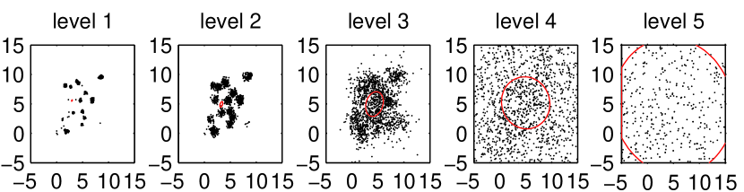
Figure 1. Simulated points of the tempered distributions over 5000 iterations. The random-walk proposal is illustrated as an ellipsoid.

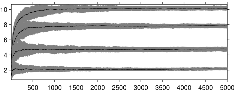
Figure 2. Convergence of the log-temperatures in the mixture example. The 10%–90% quantiles over 100 runs of the algorithm are drawn in grey and the black line shows the median.

We computed estimates of the means and the squares of the coordinates with $N=5000$ iterations of which $2500$ burn-in, and show the mean and standard deviation (in parenthesis) over 100 runs of our parallel tempering algorithm in Table 1. We considered three different random-walk adaptations: the default adaptation in (18)–(20) (Cov), with common mean and covariance estimators as defined in (23)–(24) (Cov(g)) and the RAM update defined in (25). Table 1 shows the results in the same form as [7, Table 3] to allow easy comparison. When comparing with [7], our results show smaller deviation than the unadapted parallel tempering, but bigger deviation than their samplers including also equi-energy moves. We remark that we did not adjust our algorithm at all for the example, but let the adaptation take care of that. There are no significant differences between the random-walk adaptation algorithms.

Table 1. The test of [7], Table 3 case (A) with $L=5$ temperature levels, 5000 iterations and 2500 burn-in.

	$\mathbb{E}[X_{1}]$	$\mathbb{E}[X_{2}]$	$\mathbb{E}[X_{1}^{2}]$	$\mathbb{E}[X_{2}^{2}]$
True value	4.478	4.905	25.605	33.920
Cov	4.469 (0.588)	4.950 (0.813)	25.329 (5.639)	34.209 (8.106)
Cov(g)	4.389 (0.537)	4.803 (0.692)	24.677 (5.411)	32.865 (6.660)
RAM	4.530 (0.524)	4.946 (0.811)	26.111 (5.308)	34.331 (8.292)

When looking the simulated points in Figure 1, it is clear that three temperature levels is enough to allow good mixing in the above example. We repeated the example with $L=3$ energy levels, and increased the number of iterations to $N=8333$ in order to have a comparable computational cost. The summary of the results in Table 2 indicates increased accuracy than with $L=5$ levels, and the accuracy comes close to the results reported in [7] for samplers with equi-energy moves.

Table 2. The test of [7], Table 3 case (A) with $L=3$ temperature levels, 8333 iterations and 4167 burn-in.

	$\mathbb{E}[X_{1}]$	$\mathbb{E}[X_{2}]$	$\mathbb{E}[X_{1}^{2}]$	$\mathbb{E}[X_{2}^{2}]$
True value	4.478	4.905	25.605	33.920
Cov	4.480 (0.416)	4.957 (0.571)	25.542 (4.164)	34.420 (5.669)
Cov(g)	4.488 (0.422)	4.884 (0.551)	25.719 (4.190)	33.520 (5.476)
RAM	4.490 (0.407)	4.881 (0.541)	25.667 (4.281)	33.622 (5.631)

We considered also a more difficult modification of the mixture example above. We decreased the variance of the mixture components to $\sigma^{2}=0.001$ and increased the dimension to $d=8$. The mixture means of the added coordinates were all zero. We ran our adaptive parallel tempering algorithm in this case with $L=8$ temperature levels; Table 3 summarises the results with different number of iterations. In all the cases, the first half of the iterations were burn-in. In this scenario, the different random-walk adaptation algorithms have slightly different behaviour. Particularly, the common mean and covariance estimates (Cov(g)) seem to improve over the separate covariances (Cov). The RAM approach seems to provide the most accurate results. However, we believe that this is probably due to the special properties of the example, namely the fact that all the mixture components have a common covariance, and the RAM converges close to this in the first level; see the discussion in [33].

Table 3. The root mean square errors in the modified mixture example with $\sigma^{2}=0.001$, $d=8$ and $L=8$.

$N$	Est.	Cov	Cov(g)	RAM
$10k$	$\mathbb{E}[X]$	3.080	2.245	1.660
	$\mathbb{E}[|X|^{2}]$	27.577	20.426	16.428
$20k$	$\mathbb{E}[X]$	1.788	1.580	1.429
	$\mathbb{E}[|X|^{2}]$	18.577	15.712	14.475
$40k$	$\mathbb{E}[X]$	1.439	1.267	0.952
	$\mathbb{E}[|X|^{2}]$	15.471	12.769	9.364
$80k$	$\mathbb{E}[X]$	1.257	0.975	0.698
	$\mathbb{E}[|X|^{2}]$	13.017	9.414	6.981
$160k$	$\mathbb{E}[X]$	1.096	0.680	0.508
	$\mathbb{E}[|X|^{2}]$	11.093	7.038	5.122

4.2. Spatial imaging

As another example, we consider identifying ice floes from polar satellite images as described by Banfield and Raftery [6]. The image under consideration is a 200 by 200 gray-scale satellite image, and we focus on the same 40 by 40 subregion as in [8]. The goal is to identify the presence and position of polar ice floes. Towards this goal, Higdon [14] employs a Bayesian model with an Ising model prior and following posterior distribution on $\{0,1\}^{40\times 40}$,

$$\log(\pi(x|y))\propto\sum_{1\leq i,j,\leq 40}\alpha\mathbbm{1}\{x_{i,j}=y_{i,j}\}+\sum_{(i,j)\sim(i^{\prime},j^{\prime})}\beta\mathbbm{1}\{x_{i,j}=x_{i^{\prime},j^{\prime}}\}\,,$$

where neighbourhood relation ($\sim$) is defined as vertical, horizontal and diagonal adjacencies of each pixel. Posterior distribution favours $x$ which are similar to original image $y$ (first term) and for which the neighbouring pixels are equal (second term).

In [14] and [8], the authors observed that standard MCMC algorithms which propose to flip one pixel at a time fail to explore the modes of the posterior. There are, however, some advantages of using such an algorithm, given we can overcome the difficulty in mixing between the modes. Specifically, in order to compute (the log-difference of) the unnormalised density values, we need only to explore the neighbourhoods of the pixels that have changed. Therefore, the proposal with one pixel flip at a time has a low computational cost. Moreover, such an algorithm is easy to implement.

We used our parallel tempering algorithm with the above mentioned proposal with $L=10$ temperature levels to simulate the posterior of this model with parameters $\alpha=1$ and $\beta=0.7$. We ran 100 replications of $N=100000$ iterations of the algorithm. Obtained result are shown in Figure 3 is similar to [14] and [8]. We emphasize again that our algorithm provided good results without any prior tuning.

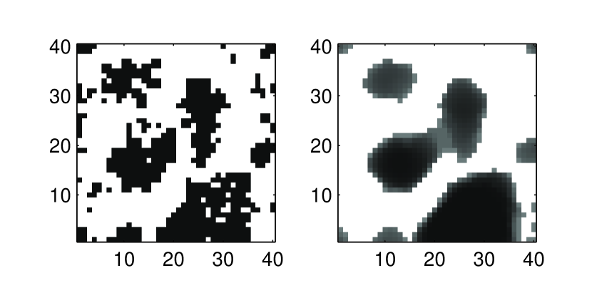
Figure 3. Spatial model example: original image (left), posterior estimate based on 100 replications of adaptive parallel tempering (right)

5. Proofs

5.1. Proof of Theorem 1

The proof follows by arguments in the literature that guarantee a geometric ergodicity for the individual random-walk Metropolis kernels, and by observing that the swap kernel is invariant under permutation-invariant functions.

We start with an easy lemma showing that a drift in cooler chain implies a drift in the higher-temperature chain.

Lemma .

Consider the drift function $W\stackrel{{\scriptstyle\mathrm{def}}}{{=}}c\pi^{-\kappa}$ for some positive constants $\kappa$ and $c$. Then, for any $\Sigma\in\mathcal{M}_{+}(d)$,

$$\beta\leq\beta^{\prime}\Longrightarrow M_{(\Sigma,\beta^{\prime})}W(x)\leq M_{(\Sigma,\beta)}W(x)\,,\quad\text{for all $x\in\mathsf{X}$ \,.}$$

Proof.

We write

$$\frac{M_{(\Sigma,\beta)}W(x)}{W(x)}=\int_{\{y\;:\;\pi(y)\geq\pi(x)\}}\left(\frac{\pi(x)}{\pi(y)}\right)^{\kappa}\;q_{\Sigma}(x-y)\mathrm{d}y\\ +\int_{\{y\;:\;\pi(y)<\pi(x)\}}\left[1-\left(\frac{\pi(y)}{\pi(x)}\right)^{\beta}+\left(\frac{\pi(y)}{\pi(x)}\right)^{\beta-\kappa}\right]q_{\Sigma}(x-y)\mathrm{d}y$$

First term is independent on $\beta$, since $\beta\mapsto 1-a^{\beta}+a^{\beta-\kappa}$ for $a\in[0,1]$ is non-increasing the second term is also non-increasing with respect to $\beta$. ∎

To control the ergodicity of each individual random-walk Metropolis sampler, it is required to have a control on the minorisation and drift constants for the kernels $M_{(\Sigma,\beta)}$. The following proposition provides such explicit control.

Lemma .

Assume (A(A1)) . Let $\varepsilon>0$ and $\beta>0$. There exist $\lambda_{\varepsilon,\beta}\in\left[0,1\right)$ and $b_{\varepsilon,\beta}<\infty$ such that for any $\Sigma\in\mathcal{M}_{+}(d,\varepsilon)$, we get

(38) $$M_{(\Sigma,\beta)}V_{\beta}\leq\lambda_{\varepsilon,\beta}V_{\beta}+b_{\varepsilon,\beta}\,,$$

where $V_{\beta}\stackrel{{\scriptstyle\mathrm{def}}}{{=}}(\pi/\left\|\pi\right\|_{\infty})^{-\beta/2}$, where $\left\|\pi\right\|_{\infty}=\sup_{x\in\mathsf{X}}\pi(x)$.

Proof.

It is easily seen that if the target distribution is super-exponential in the tails (A(A1)) , then all the tempered versions $\pi^{\beta}/Z(\beta)$, where the normalising constant $Z(\beta)$ is defined in (2), satisfy (A(A1)) as well.

The result then follows from Andrieu and Moulines [1, Proposition 12]. ∎

Proposition .

Assume (A(A1)) and let $\epsilon>0$ and $\beta_{0}>0$. Then, there exists $\lambda_{\epsilon,\beta_{0}}<1$, and $b_{\epsilon,\beta_{0}}<\infty$ such that, for all $\boldsymbol{\Sigma}\in\mathcal{M}^{L}_{+}(d,\epsilon)$ and $\boldsymbol{\beta}\in\mathcal{K}_{\beta_{0}}$,

(39) $$\mathbf{M}_{(\boldsymbol{\Sigma},\boldsymbol{\beta})}\mathbf{V}_{\beta_{0}}\leq\lambda_{\epsilon,\beta_{0}}\mathbf{V}_{\beta_{0}}+b_{\epsilon,\beta_{0}}\,,$$

(40) $$\mathbf{S}_{\boldsymbol{\beta}}\mathbf{V}_{\beta_{0}}=\mathbf{V}_{\beta_{0}}\,,$$

(41) $$\mathbf{P}_{(\boldsymbol{\Sigma},\boldsymbol{\beta})}\mathbf{V}_{\beta_{0}}\leq\lambda_{\epsilon,\beta_{0}}\mathbf{V}_{\beta_{0}}+b_{\epsilon,\beta_{0}}\,,$$

Proof.

By subsection 5.1, since $\boldsymbol{\beta}\in\mathcal{K}_{\beta_{0}}$, we get

(42) $$\mathbf{M}_{(\boldsymbol{\Sigma},\boldsymbol{\beta})}\mathbf{V}_{\beta_{0}}(x^{(1:L)}) =\sum_{\ell=1}^{L}M_{(\Sigma^{(\ell)},\beta^{(\ell)})}V_{\beta_{0}}(x^{(\ell)})$$

$$\leq\sum_{\ell=1}^{L}M_{(\Sigma^{(\ell)},\beta_{0})}V_{\beta_{0}}(x^{(\ell)})\,.$$

Then, by subsection 5.1, since $\boldsymbol{\Sigma}\in\mathcal{M}_{+}(d,\epsilon)$, it holds

$$\sum_{\ell=1}^{L}M_{(\Sigma^{(\ell)},\beta_{0})}V_{\beta_{0}}(x^{(\ell)})\leq\lambda_{\epsilon,\beta_{0}}\sum_{\ell=1}^{L}V_{\beta_{0}}(x^{(\ell)})+Lb_{\epsilon,\beta_{0}}\,.$$

Thanks to the definition of the swapping kernel (8)–(10), for any positive measurable function $F:\mathsf{X}^{L}\to\mathbb{R}_{+}$ which is invariant by permutation, we get $\mathbf{S}_{\boldsymbol{\beta}}F(x^{(1:L)})=F(x^{(1:L)})$. Since the drift function $\mathbf{V}_{\beta_{0}}$ defined in (30) is invariant by permutation we obtain

$$\mathbf{S}_{\boldsymbol{\beta}}\left[\lambda_{\epsilon,\beta_{0}}\mathbf{V}_{\beta_{0}}(x^{(1:L)})+Lb_{\epsilon,\beta_{0}}\right] =\lambda_{\epsilon,\beta_{0}}\mathbf{S}_{\boldsymbol{\beta}}\mathbf{V}_{\beta_{0}}(x^{(1:L)})+Lb_{\epsilon,\beta_{0}}$$

$$=\lambda_{\epsilon,\beta_{0}}\mathbf{V}_{\beta_{0}}(x^{(1:L)})+Lb_{\epsilon,\beta_{0}}\,.\qed$$

Proposition .

Assume (A(A1)) . Let $\epsilon>0$, $\beta_{0}>0$ and $r>1$, and consider the level set $\mathsf{C}_{r}\stackrel{{\scriptstyle\mathrm{def}}}{{=}}\{\mathbf{x}\in\mathsf{X}^{L}\,:\,\mathbf{V}_{\beta_{0}}(\mathbf{x})\leq r\}$. There exists a constant $\delta_{r,\epsilon,\beta_{0}}>0$ such that for all $\boldsymbol{\Sigma}\in\mathcal{M}_{+}(d,\epsilon)$ and $\boldsymbol{\beta}\in\mathcal{K}_{\beta_{0}}$, the set $\mathsf{C}_{r}$ is a $(1,\delta_{r,\epsilon,\beta_{0}},\nu_{r})$-small set for $\mathbf{P}_{(\boldsymbol{\Sigma},\boldsymbol{\beta})}$, that is,

(43) $$\mathbf{P}_{(\boldsymbol{\Sigma},\boldsymbol{\beta})}(\mathbf{x},\cdot)\geq\delta_{r,\epsilon,\beta_{0}}\nu_{r,\epsilon,\beta_{0}}(\cdot)\quad\mathbf{x}\in\mathsf{C}_{r},$$

where $\nu_{r}(\cdot)=\lambda^{\mathrm{Leb}}(\cdot\cap\mathsf{C}_{r})/\lambda^{\mathrm{Leb}}(\mathsf{C}_{r})$ is a probability measure on $\mathsf{C}_{r}$ and $\lambda^{\mathrm{Leb}}$ stands for the Lebesgue measure.

Proof.

It is easy to see that the set $\mathsf{C}_{r}$ is absorbing for $\mathbf{S}_{\boldsymbol{\beta}}$ because $\mathbf{S}_{\boldsymbol{\beta}}V_{\boldsymbol{\beta}}(x)=V_{\boldsymbol{\beta}}(x)$ as observed in the proof of subsection 5.1, implying $\mathbf{S}_{\boldsymbol{\beta}}(x,\mathsf{C}_{r})=1$ for all $x\in\mathsf{C}_{r}$. Hence for $x\in\mathsf{C}_{r}$

(44) $$\mathbf{P}_{(\boldsymbol{\Sigma},\boldsymbol{\beta})}(\mathbf{x},\mathsf{A})\geq\int_{\mathsf{C}_{r}\cap\mathsf{A}}\prod_{\ell=1}^{L}\left(1\wedge\frac{\pi(y^{(\ell)})}{\pi(x^{(\ell)})}\right)^{\beta^{(\ell)}}q_{\Sigma^{(\ell)}}(y^{(\ell)}-x^{(\ell)})\mathrm{d}y^{(1:L)}\,,$$

where $q_{\Sigma}$ is the multivariate Gaussian density with zero mean and covariance $\Sigma$. Since the set $\mathsf{C}_{r}$ is compact and $\boldsymbol{\Sigma}\in\mathcal{M}^{L}_{+}(\beta_{0},\epsilon)$, there exists a constant $C_{r,\epsilon,\beta_{0}}>0$ such that for any $\ell=1,\dots,L$

$$\inf_{(x,y)\in\mathsf{C}_{r}\times\mathsf{C}_{r}}q^{(\ell)}(y^{(\ell)}-x^{(\ell)})\geq C_{r,\epsilon,\beta_{0}}\,.$$

Therefore, by (44) and since $\beta^{(\ell)}\in(0,1]$, we obtain for $x\in\mathsf{C}_{r}$

$$\mathbf{P}_{(\boldsymbol{\Sigma},\boldsymbol{\beta})}(\mathbf{x},\mathsf{A}) \geq C_{r,\epsilon,\beta_{0}}^{L}\int_{\mathsf{C}_{r}\cap\mathsf{A}}\prod_{\ell=1}^{L}\left(1\wedge\frac{\pi(y^{(\ell)})}{\pi(x^{(\ell)})}\right)\mathrm{d}y^{(1:L)}\,.$$

If $y=(y^{(1:L)})\in\mathsf{C}_{r}$, we get $(\pi(y^{(\ell)})/\left\|\pi\right\|_{\infty})^{-\beta_{0}}\leq r/L$ for all $\ell\in\{1,\dots,L\}$, which implies that $(L/r)^{2/\beta_{0}}\left\|\pi\right\|_{\infty}\leq\pi(y)$. Hence, for all $(x,y)\in C_{r}\times C_{r}$, $\pi(y)/\pi(x)\leq(L/r)^{2/\beta_{0}}$, showing that

$$\mathbf{P}_{(\boldsymbol{\Sigma},\boldsymbol{\beta})}(\mathbf{x},\mathsf{A})\geq C_{r,\epsilon,\beta_{0}}^{L}\left[(1\wedge(L/r))^{2/\beta_{0}}\right]^{L}\lambda^{\mathrm{Leb}}(C_{r})\lambda^{\mathrm{Leb}}_{C_{r}}(\mathsf{C}_{r}\cap\mathsf{A})\,,$$

where $\lambda^{\mathrm{Leb}}_{\mathsf{C}_{r}}(\cdot)=\lambda^{\mathrm{Leb}}(\mathsf{C}_{r}\cap\cdot)/\lambda^{\mathrm{Leb}}(\mathsf{C}_{r})$. ∎

Proof of Theorem 1.

Choose a sufficiently large $r>1$ so that there exists a $\tilde{\lambda}_{\epsilon,\beta_{0}}<1$ such that

$$\mathbf{P}_{(\boldsymbol{\Sigma},\boldsymbol{\beta})}\mathbf{V}_{\beta_{0}}(x)\leq\lambda_{\epsilon,\beta_{0}}\mathbf{V}_{\beta_{0}}(x)+\mathbbm{I}\left\{x\notin C\right\}b_{\epsilon,\beta_{0}}$$

by subsection 5.1, where $\mathsf{C}_{r}$ is defined in subsection 5.1. This drift inequality, with the minorisation inequality in subsection 5.1 imply $V$-uniform ergodicity (33) with constants depending only on $\tilde{\lambda}_{\epsilon,\beta_{0}}<1$, $b_{\epsilon,\beta_{0}}$ and $\delta_{r,\epsilon,\beta_{0}}$ [e.g. 23]. ∎

5.2. Proof of Theorem 2

We preface the proof of this Theorem by several technical lemmas.

Lemma .

For all $(\beta,\beta^{\prime})\in\left(0,1\right)^{2}$ we have

$$\sup_{z\in\left[0,1\right]}|z^{\beta}-z^{\beta^{\prime}}|\leq\frac{1}{\max\{\beta,\beta^{\prime}\}}|\beta^{\prime}-\beta|\,.$$

Proof.

Without loss of generality, assume that $0<\beta<\beta^{\prime}<1$. The function $w:\left[0,1\right]\to\mathbb{R}$ defined as $w(z)=z^{\beta}-z^{\beta^{\prime}}$ is continuous, non-negative and $w(0)=w(1)=0$. Therefore, the maximum of this function is obtained inside the interval $(0,1)$. By computing the derivative $w^{\prime}(z)=\beta z^{\beta-1}-\beta^{\prime}z^{\beta^{\prime}-1}$ and setting $w^{\prime}(z)=0$, we find the maximum at $z=\big{(}\frac{\beta}{\beta^{\prime}}\big{)}^{1/(\beta^{\prime}-\beta)}$, so

$$\sup_{z\in\left[0,1\right]}|z^{\beta}-z^{\beta^{\prime}}|=\left(\frac{\beta}{\beta^{\prime}}\right)^{\frac{\beta}{\beta^{\prime}-\beta}}\left(1-\frac{\beta}{\beta^{\prime}}\right)\leq\left(1-\frac{\beta}{\beta^{\prime}}\right)=\frac{1}{\beta^{\prime}}(\beta^{\prime}-\beta)\,.\qed$$

Lemma .

Set $\beta_{0}\in\left(0,1\right]$. There exists a constant $K_{\beta_{0}}<\infty$ such that for any $(\beta,\beta^{\prime})\in\left[\beta_{0},1\right]^{2}$, any covariance matrix $\Sigma\in\mathcal{M}_{+}(d)$,

(45) $$\int_{\mathsf{X}}\left(V_{\beta_{0}}(y)+V_{\beta_{0}}(x)\right)\left|\alpha_{\beta}(x,y)-\alpha_{\beta^{\prime}}(x,y)\right|q_{\Sigma}(y-x)\lambda^{\mathrm{Leb}}(\mathrm{d}y)\\ \leq K_{\beta_{0}}|\beta-\beta^{\prime}|V_{\beta_{0}}(x)\,.$$

In addition, for any measurable function $g$ with $\left\|g\right\|_{V_{\beta_{0}}}\leq 1$,

(46) $$\left|M_{(\Sigma,\beta)}g(x)-M_{(\Sigma,\beta^{\prime})}g(x)\right|\leq K_{\beta_{0}}|\beta-\beta^{\prime}|V_{\beta_{0}}(x)\,.$$

Proof.

Without loss of generality, we assume that $\beta<\beta^{\prime}$. Recall that $V_{\beta_{0}}(y)\propto\pi^{-\beta_{0}/2}(y)$. Note that

$$\int_{\mathsf{X}}V_{\beta_{0}}(y)\left|\alpha_{\beta}(x,y)-\alpha_{\beta^{\prime}}(x,y)\right|q_{\Sigma}(y-x)\mathrm{d}y\\ =V_{\beta_{0}}(x)\int_{\mathsf{R}_{x}}\left|\left(\frac{\pi(y)}{\pi(x)}\right)^{\beta-\beta_{0}/2}-\left(\frac{\pi(y)}{\pi(x)}\right)^{\beta^{\prime}-\beta_{0}/2}\right|q_{\Sigma}(y-x)\mathrm{d}y\,,$$

where $\mathsf{R}_{x}\mathrel{\mathop{:}}=\{y\in\mathsf{X}:\pi(y)<\pi(x)\}$, and

$$V_{\beta_{0}}(x)\int_{\mathsf{X}}\left|\alpha_{\beta}(x,y)-\alpha_{\beta^{\prime}}(x,y)\right|q_{\Sigma}(y-x)\mathrm{d}y\\ =V_{\beta_{0}}(x)\int_{\mathsf{R}_{x}}\left|\left(\frac{\pi(y)}{\pi(x)}\right)^{\beta}-\left(\frac{\pi(y)}{\pi(x)}\right)^{\beta^{\prime}}\right|q_{\Sigma}(y-x)\mathrm{d}y\,.$$

Using subsection 5.2, we get

$$\int_{\mathsf{R}_{x}}\left|\left(\frac{\pi(y)}{\pi(x)}\right)^{\beta-\beta_{0}/2}-\left(\frac{\pi(y)}{\pi(x)}\right)^{\beta^{\prime}-\beta_{0}/2}\right|q_{\Sigma}(y-x)\mathrm{d}y\leq\frac{1}{\beta-\beta_{0}/2}|\beta^{\prime}-\beta|\,,$$

and similarly

$$\int_{\mathsf{R}_{x}}\left|\left(\frac{\pi(y)}{\pi(x)}\right)^{\beta}-\left(\frac{\pi(y)}{\pi(x)}\right)^{\beta^{\prime}}\right|q_{\Sigma}(y-x)\mathrm{d}y\leq\frac{1}{\beta}|\beta^{\prime}-\beta|\,,$$

which concludes the proof of (45).

We consider now (46). Note that

(47) $$\left|M_{(\Sigma,\beta)}g(x)-M_{(\Sigma,\beta^{\prime})}g(x)\right|$$

$$=\left|\int_{\mathsf{X}}\left(g(y)-g(x)\right)\left(\alpha_{\beta}(x,y)-\alpha_{\beta^{\prime}}(x,y)\right)q_{\Sigma}(y-x)\mathrm{d}y\right|$$

$$\leq\int_{\mathsf{X}}\left|g(y)-g(x)\right|\left|\alpha_{\beta}(x,y)-\alpha_{\beta^{\prime}}(x,y)\right|q_{\Sigma}(y-x)\mathrm{d}y$$

$$\leq\int_{\mathsf{X}}\left(V_{\beta_{0}}(y)+V_{\beta_{0}}(x)\right)\left|\alpha_{\beta}(x,y)-\alpha_{\beta^{\prime}}(x,y)\right|q_{\Sigma}(y-x)\mathrm{d}y$$

and we conclude using (45). ∎

The following result is a restatement of [1, Proposition 12 and (the proof of) Lemma 13].

Lemma .

For any $\epsilon>0$ there exists $K_{\epsilon}<\infty$ such that for any $(\Sigma,\Sigma^{\prime})\in\mathcal{M}_{+}(d,\epsilon)$, $\beta\in[0,1]$, and function $g$ with $\|g\|_{V_{\beta_{0}}}\leq 1$, we have

$$\left|M_{(\Sigma,\beta)}g(x)-M_{(\Sigma^{\prime},\beta)}g(x)\right|\leq K_{\epsilon}|\Sigma-\Sigma^{\prime}|V_{\beta_{0}}(x)\,.$$

In addition there exists $K_{q}<\infty$ such that

(48) $$\int_{\mathsf{X}}|q_{\Sigma}(z)-q_{\Sigma^{\prime}}(z)|\mathrm{d}z\leq K_{q}|\Sigma-\Sigma^{\prime}|.$$

subsection 5.2 can be generalised also for non-Gaussian proposal distributions, including the multivariate Student [31, Appendix B].

Now we show the local Lipschitz-continuity of the mapping $(\boldsymbol{\Sigma},\boldsymbol{\beta})\mapsto\mathbf{M}_{(\boldsymbol{\Sigma},\boldsymbol{\beta})}$.

Proposition .

Assume (A(A1)) . Let $\epsilon>0$ and $\beta_{0}>0$, and $\eta>0$. There exists a constant $K_{\epsilon,\beta_{0},\eta}<\infty$ such that such that for all $\boldsymbol{\Sigma},\boldsymbol{\Sigma}^{\prime}\in\mathcal{M}^{L}_{+}(d,\epsilon)$, $\boldsymbol{\beta},\boldsymbol{\beta}^{\prime}\in\mathcal{K}_{\beta_{0},\eta}$, and functions $g$ with $\left\|g\right\|_{\mathbf{V}_{\beta_{0}}}\leq 1$, we have

$$\left|\mathbf{M}_{(\boldsymbol{\Sigma},\boldsymbol{\beta})}g(\mathbf{x})-\mathbf{M}_{(\boldsymbol{\Sigma}^{\prime},\boldsymbol{\beta}^{\prime})}g(\mathbf{x})\right|\leq K_{\epsilon,\beta_{0},\eta}\left\{|\boldsymbol{\beta}-\boldsymbol{\beta}^{\prime}|+|\boldsymbol{\Sigma}-\boldsymbol{\Sigma}^{\prime}|\right\}\mathbf{V}_{\beta_{0}}(\mathbf{x})\,.$$

Remark .

In this proof, it is possible to set $\eta=0$. The use of $\eta>0$ is required in the proof of continuity.

Proof.

We may write

(49) $$\left|\mathbf{M}_{(\boldsymbol{\Sigma},\boldsymbol{\beta})}g(\mathbf{x})-\mathbf{M}_{(\boldsymbol{\Sigma}^{\prime},\boldsymbol{\beta}^{\prime})}g(\mathbf{x})\right|\leq\left|\mathbf{M}_{(\boldsymbol{\Sigma},\boldsymbol{\beta})}g(\mathbf{x})-\mathbf{M}_{(\boldsymbol{\Sigma},\boldsymbol{\beta}^{\prime})}g(\mathbf{x})\right|\\ +\left|\mathbf{M}_{(\boldsymbol{\Sigma},\boldsymbol{\beta}^{\prime})}g(\mathbf{x})-\mathbf{M}_{(\boldsymbol{\Sigma}^{\prime},\boldsymbol{\beta}^{\prime})}g(\mathbf{x})\right|\stackrel{{\scriptstyle\mathrm{def}}}{{=}}R_{1}(\mathbf{x})+R_{2}(\mathbf{x})\,.$$

First, we consider $R_{1}$. We prove by induction that there exists a constant $K_{k,\epsilon,\beta_{0},\eta}<\infty$ such that, for all measurable $g$ such that $\left\|g\right\|_{\mathbf{V}_{\beta_{0}}}\leq 1$,

(50) $$\left|\mathbf{M}^{(k)}_{(\boldsymbol{\Sigma},\boldsymbol{\beta})}g(\mathbf{x})-\mathbf{M}^{(k)}_{(\boldsymbol{\Sigma},\boldsymbol{\beta}^{\prime})}g(\mathbf{x})\right|\leq K_{k,\epsilon,\beta_{0},\eta}|\boldsymbol{\beta}-\boldsymbol{\beta}^{\prime}|\mathbf{V}_{\beta_{0}}(\mathbf{x})\,,$$

where $\mathbf{M}^{(k)}_{(\boldsymbol{\Sigma},\boldsymbol{\beta})}\stackrel{{\scriptstyle\mathrm{def}}}{{=}}\prod_{1\leq\ell\leq k}\check{M}_{(\Sigma^{(\ell)},\beta^{(\ell)})}$, and

$$\check{M}_{(\Sigma^{(\ell)},\beta^{(\ell)})}(x^{(1:L)},A_{1}\times\cdots\times A_{L})\stackrel{{\scriptstyle\mathrm{def}}}{{=}}M_{(\Sigma^{(\ell)},\beta^{(\ell)})}(x^{(\ell)},A_{\ell})\prod_{i\neq\ell}\delta_{x^{(i)}}(A_{i}).$$

We first establish the result for $k=1$. For any $\ell\in\{1,\dots,L\}$, we get

$$\left|\check{M}_{(\Sigma^{(\ell)},\beta^{(\ell)})}g(\mathbf{x})-\check{M}_{(\Sigma^{(\ell)},\beta^{\prime(\ell)})}g(\mathbf{x})\right|$$

$$\leq\int_{\mathsf{X}}\left|g(x^{(1:\ell-1)},y,x^{(\ell+1:L)})-g(x^{(1:L)})\right|$$

$$\phantom{=\int_{X}set()}\left|\alpha_{\beta^{(\ell)}}(x^{(\ell)},y)-\alpha_{\beta^{\prime(\ell)}}(x^{(\ell)},y)\right|q_{\Sigma^{(\ell)}}(y-x^{(\ell)})\mathrm{d}y$$

$$\leq\int_{\mathsf{X}}\left(V_{\beta_{0}}(y)+V_{\beta_{0}}(x^{(\ell)})+2\sum_{k\neq\ell}V_{\beta_{0}}(x^{(k)})\right)$$

$$\phantom{=\int_{X}set()}\left|\alpha_{\beta^{(\ell)}}(x^{(\ell)},y)-\alpha_{\beta^{\prime(\ell)}}(x^{(\ell)},y)\right|q_{\Sigma^{(\ell)}}(y-x^{(\ell)})\mathrm{d}y$$

Applying (45), there exists $K<\infty$ such that for any $\ell\in\{1,\dots,L\}$, we get

(51) $$\left|\check{M}_{(\Sigma^{(\ell)},\beta^{(\ell)})}g(\mathbf{x})-\check{M}_{(\Sigma^{(\ell)},\beta^{\prime(\ell)})}g(\mathbf{x})\right|\leq K|\beta^{(\ell)}-\beta^{\prime(\ell)}|\sum_{k=1}^{L}V_{\beta_{0}}(x^{(k)})$$

Taking $\ell=1$ establishes (50) with $k=1$. Assume now that (50) is satisfied for some $k\in\{2,\dots,L-1\}$. We have

$$\big{|}\mathbf{M}^{(k+1)}_{(\boldsymbol{\Sigma},\boldsymbol{\beta})}g(\mathbf{x}) -\mathbf{M}^{(k+1)}_{(\boldsymbol{\Sigma},\boldsymbol{\beta}^{\prime})}g(\mathbf{x})\big{|}$$

$$\leq\big{|}\left(\check{M}_{(\Sigma^{(k+1)},\beta^{(k+1)})}-\check{M}_{(\Sigma^{(k+1)},\beta^{\prime(k+1)})}\right)\mathbf{M}^{(k)}_{(\boldsymbol{\Sigma},\boldsymbol{\beta})}g(\mathbf{x})\big{|}$$

$$\phantom{\leq}+\big{|}\check{M}_{(\Sigma^{(k+1)},\beta^{\prime(k+1)})}\big{(}\mathbf{M}^{(k)}_{(\boldsymbol{\Sigma},\boldsymbol{\beta})}-\mathbf{M}^{(k)}_{(\boldsymbol{\Sigma},\boldsymbol{\beta}^{\prime})}\big{)}g(\mathbf{x})\big{|}$$

For any $\left\|g\right\|_{\mathbf{V}_{\beta_{0}}}\leq 1$, we have

$$\big{|}\mathbf{M}^{(k)}_{(\boldsymbol{\Sigma},\boldsymbol{\beta})}g(\mathbf{x})\big{|}\leq\mathbf{M}^{(k)}_{(\boldsymbol{\Sigma},\boldsymbol{\beta})}\mathbf{V}_{\beta_{0}}(\mathbf{x})=\sum_{\ell=1}^{k}M_{(\Sigma^{(\ell)},\beta^{(\ell)})}V_{\beta_{0}}(x^{(\ell)})+\sum_{\ell=k+1}^{L}V_{\beta_{0}}(x^{(\ell)})\,.$$

subsection 5.1 implies that, for any $\left\|g\right\|_{\mathbf{V}_{\beta_{0}}}\leq 1$,

$$\big{|}\mathbf{M}^{(k)}_{(\boldsymbol{\Sigma},\boldsymbol{\beta})}g(\mathbf{x})\big{|}\leq\mathbf{V}_{\beta_{0}}(\mathbf{x})+kb_{\epsilon,\beta_{0}}\,,$$

showing that $\|\mathbf{M}^{(k)}_{(\boldsymbol{\Sigma},\boldsymbol{\beta})}g\|_{\mathbf{V}_{\beta_{0}}}<\infty$. Hence by (51) there exists a constant $K^{(1)}_{k+1,\epsilon,\beta_{0},\eta}<\infty$ such that

$$\big{|}\big{(}\check{M}_{(\Sigma^{(k+1)},\beta^{(k+1)})}-\check{M}_{(\Sigma^{(k+1)},\beta^{\prime(k+1)})}\big{)}\mathbf{M}^{(k)}_{(\boldsymbol{\Sigma},\boldsymbol{\beta})}g(\mathbf{x})\big{|}\\ \leq K^{(1)}_{k+1,\epsilon,\beta_{0},\eta}\;|\beta^{(k+1)}-\beta^{\prime(k+1)}|\mathbf{V}_{\beta_{0}}(\mathbf{x})\,.$$

By the induction assumption (50) and subsection 5.1 there exists $K^{(2)}_{k+1,\epsilon,\beta_{0},\eta}<\infty$ such that second term is bounded by

$$\big{|}M_{(\Sigma^{(k+1)},\beta^{\prime(k+1)})}\big{(}\mathbf{M}^{(k)}_{(\boldsymbol{\Sigma},\boldsymbol{\beta})}-\mathbf{M}^{(k)}_{(\boldsymbol{\Sigma},\boldsymbol{\beta}^{\prime})}\big{)}g(\mathbf{x})\big{|}\\ \leq K_{k,\epsilon,\beta_{0},\eta}|\boldsymbol{\beta}-\boldsymbol{\beta}^{\prime}|M_{(\Sigma^{(k+1)},\beta^{\prime(k+1)})}\mathbf{V}_{\beta_{0}}(\mathbf{x})\leq K^{(2)}_{k+1,\epsilon,\beta_{0},\eta}|\boldsymbol{\beta}-\boldsymbol{\beta}^{\prime}|\mathbf{V}_{\beta_{0}}(\mathbf{x})\,.$$

This shows that (50) is satisfied for $k+1$. Carrying out the induction until $k=L$, there exists a constant $K_{L,\epsilon,\beta_{0},\eta}<\infty$ such that, for all $\left\|g\right\|_{\mathbf{V}_{\beta_{0}}}\leq 1$,

(52) $$R_{1}(x)=\left|\mathbf{M}_{(\boldsymbol{\Sigma},\boldsymbol{\beta})}g(\mathbf{x})-\mathbf{M}_{(\boldsymbol{\Sigma},\boldsymbol{\beta}^{\prime})}g(\mathbf{x})\right|\leq K_{L,\epsilon,\beta_{0},\eta}|\boldsymbol{\beta}-\boldsymbol{\beta}^{\prime}|\mathbf{V}_{\beta_{0}}(\mathbf{x})\,,$$

where $R_{1}$ is defined in (49).

Consider now $R_{2}$. It is easy to see that by (48) we obtain analogous formula to (51); that is, with the same temperatures $\boldsymbol{\beta}$ but different covariance matrices $\boldsymbol{\Sigma}$ and $\boldsymbol{\Sigma}^{\prime}$. The proof is concluded by using the same induction proof as for the term $R_{1}$. ∎

Lemma .

Let $\beta_{0}>0$ and $\eta>0$. Then, there exists a constant $K_{\beta_{0},\eta}$ such that, for any $\boldsymbol{\beta},\boldsymbol{\beta}^{\prime}\in\mathcal{K}_{\beta_{0},\eta}$ and for any measurable function $g$ with $\left\|g\right\|_{\mathbf{V}_{\beta_{0}}}\leq 1$, it holds that

$$|\mathbf{S}_{\boldsymbol{\beta}}g(\mathbf{x})-\mathbf{S}_{\boldsymbol{\beta}^{\prime}}g(\mathbf{x})|\leq K_{\beta_{0},\eta}|\boldsymbol{\beta}-\boldsymbol{\beta}^{\prime}|\mathbf{V}_{\beta_{0}}(\mathbf{x})\,.$$

Proof.

Using the definition (8) of $\mathbf{S}_{\boldsymbol{\beta}}$, we get

(53) $$|\mathbf{S}_{\boldsymbol{\beta}}g(\mathbf{x})-\mathbf{S}_{\boldsymbol{\beta}^{\prime}}g(\mathbf{x})|=\frac{1}{L-1}\Big{|}\sum_{\ell=1}^{L-1}\left(\varpi^{(\ell)}_{\boldsymbol{\beta}}(x^{(\ell)},x^{(\ell+1)})-\varpi^{(\ell)}_{\boldsymbol{\beta}^{\prime}}(x^{(\ell)},x^{(\ell+1)})\right)\\ \times\left(g(x^{(1:\ell-1)},x^{(\ell+1)},x^{(\ell)},\dots,x^{(L)})-g(x^{(1:\ell-1)},x^{(\ell)},x^{(\ell+1)},\dots,x^{(L)})\right)\Big{|}\,.$$

By (9), it holds that $\varpi^{(\ell)}_{\boldsymbol{\beta}}(x^{(\ell)},x^{(\ell+1)})=\varpi^{(\ell)}_{\boldsymbol{\beta}^{\prime}}(x^{(\ell)},x^{(\ell+1)})=1$ whenever $\pi(x^{(\ell+1)})\geq\pi(x^{(\ell)})$. Therefore, using subsection 5.2, we get that

(54) $$\big{|}\varpi^{(\ell)}_{\boldsymbol{\beta}}(x^{(\ell)},x^{(\ell+1)})-\varpi^{(\ell)}_{\boldsymbol{\beta}^{\prime}}(x^{(\ell)},x^{(\ell+1)})\big{|}$$

$$=\mathbbm{1}_{\{\pi(x^{(\ell+1)})\leq\pi(x^{(\ell)})\}}\left|\left(\frac{\pi(x^{(\ell+1)})}{\pi(x^{(\ell)})}\right)^{\beta^{(\ell)}-\beta^{(\ell+1)}}-\left(\frac{\pi(x^{(\ell+1)})}{\pi(x^{(\ell)})}\right)^{\beta^{\prime(\ell)}-\beta^{\prime(\ell+1)}}\right|$$

$$\leq\frac{|\beta^{(\ell+1)}-\beta^{\prime(\ell+1)}|+|\beta^{(\ell)}-\beta^{\prime(\ell)}|}{\left(\beta^{(\ell)}-\beta^{(\ell+1)}\right)\wedge\left(\beta^{\prime(\ell)}-\beta^{\prime(\ell+1)}\right)}\,.$$

Since $\boldsymbol{\beta},\boldsymbol{\beta}^{\prime}\in\mathcal{K}_{\beta_{0},\eta}$, $\max\{\left(\beta^{(\ell)}-\beta^{(\ell+1)}\right),\left(\beta^{\prime(\ell)}-\beta^{\prime(\ell+1)}\right)\}\geq\eta$ for all $\ell\in\{1,\dots,L\}$. Because $\left\|g\right\|_{\mathbf{V}_{\beta_{0}}}\leq 1$ and $\mathbf{V}_{\beta_{0}}$ are invariant under permutations, we have by (53) and (54)

$$|\mathbf{S}_{\boldsymbol{\beta}}g(\mathbf{x})-\mathbf{S}_{\boldsymbol{\beta}^{\prime}}g(\mathbf{x})|\leq\frac{4}{(L-1)\eta}\mathbf{V}_{\beta_{0}}(\mathbf{x})\sum_{\ell=1}^{L}|\beta^{(\ell)}-\beta^{\prime(\ell)}|\,.\qed$$

Now we are ready to conclude with the continuity of the parallel tempering kernels.

Proof of Theorem 2.

The definition (30) of $\mathbf{V}_{\boldsymbol{\beta}_{0}}$ implies that, for any $\alpha\in\left(0,1\right]$,

$$L^{\alpha-1}\sum_{i=1}^{L}V_{\alpha\beta_{0}}(x^{(i)})\leq\left(\sum_{i=1}^{L}V_{\beta_{0}}(x^{(i)})\right)^{\alpha}\leq\sum_{i=1}^{L}V_{\alpha\beta_{0}}(x^{(i)})\,,$$

showing that $L^{\alpha-1}\mathbf{V}_{\alpha\beta_{0}}(\mathbf{x})\leq\mathbf{V}^{\alpha}_{\beta_{0}}(\mathbf{x})\leq\mathbf{V}_{\alpha\beta_{0}}(\mathbf{x})$. Therefore, the norms $\left\|\cdot\right\|_{\mathbf{V}^{\alpha}_{\beta_{0}}}$ and $\left\|\cdot\right\|_{\mathbf{V}_{\alpha\beta_{0}}}$ are equivalent. It suffices to prove the results with $\alpha=1$. Write

$$|\mathbf{P}_{(\boldsymbol{\Sigma},\boldsymbol{\beta})}g(\mathbf{x})-\mathbf{P}_{(\boldsymbol{\Sigma}^{\prime},\boldsymbol{\beta}^{\prime})}g(\mathbf{x})|\leq T_{1}(\mathbf{x})+T_{2}(\mathbf{x})\,,$$

where

$$T_{1}(\mathbf{x}) \stackrel{{\scriptstyle\mathrm{def}}}{{=}}\left|\mathbf{S}_{\boldsymbol{\beta}}(\mathbf{M}_{(\boldsymbol{\Sigma},\boldsymbol{\beta})}-\mathbf{M}_{(\boldsymbol{\Sigma}^{\prime},\boldsymbol{\beta}^{\prime})})g(\mathbf{x})\right|$$

$$T_{2}(\mathbf{x}) \stackrel{{\scriptstyle\mathrm{def}}}{{=}}\left|(\mathbf{S}_{\boldsymbol{\beta}}-\mathbf{S}_{\boldsymbol{\beta}^{\prime}})\mathbf{M}_{(\boldsymbol{\Sigma}^{\prime},\boldsymbol{\beta}^{\prime})}g(\mathbf{x})\right|\,.$$

By subsection 5.2, we obtain

$$T_{1}(\mathbf{x})\leq K_{\epsilon,\beta_{0},\eta}\left\{|\boldsymbol{\beta}-\boldsymbol{\beta}^{\prime}|+|\boldsymbol{\Sigma}-\boldsymbol{\Sigma}^{\prime}|\right\}\mathbf{S}_{\boldsymbol{\beta}}\mathbf{V}_{\beta_{0}}(\mathbf{x})\\ \leq K_{\epsilon,\beta_{0},\eta}\,\left\{|\boldsymbol{\beta}-\boldsymbol{\beta}^{\prime}|+|\boldsymbol{\Sigma}-\boldsymbol{\Sigma}^{\prime}|\right\}\mathbf{V}_{\beta_{0}}(\mathbf{x})\,.$$

By (39) of subsection 5.1, we obtain that $\left\|\mathbf{M}_{(\boldsymbol{\Sigma}^{\prime},\boldsymbol{\beta}^{\prime})}g\right\|_{\mathbf{V}_{\beta_{0}}}\leq C$. Hence, by subsection 5.2 we get that

$$T_{2}(\mathbf{x})\leq CK_{\beta_{0},\eta}|\boldsymbol{\beta}-\boldsymbol{\beta}^{\prime}|\mathbf{V}_{\beta_{0}}(\mathbf{x})\,,$$

which concludes the proof. ∎

5.3. Proof of Theorem 3

We now turn into the proof of the strong law of large numbers. We start by gathering some known results and by technical lemmas.

Lemma .

Assume (A(A1)) and that, in addition, $\mathbb{E}\left[\mathbf{V}_{\beta_{0}}(\mathbf{X}_{0})\right]<\infty$. Then,

$$\sup_{n\geq 1}\mathbb{E}\left[\mathbf{V}_{\beta_{0}}(\mathbf{X}_{n})\right]<\infty\,,$$

where $\mathbf{X}_{n}$ is the state of the adaptive parallel tempering algorithm defined in (4).

Proof.

Under (A(A1)) , by subsection 5.1, for all $n\in\mathbb{N}$ we have that

(55) $$\mathbf{P}_{(\boldsymbol{\Sigma}_{n},\boldsymbol{\beta}_{n})}\mathbf{V}_{\beta_{0}}\leq\lambda_{\epsilon,\beta_{0}}\mathbf{V}_{\beta_{0}}+b\,.$$

Iterating (55), by (27) we obtain

$$\mathbb{E}[\mathbf{V}_{\beta_{0}}(\mathbf{X}_{n})]=\mathbb{E}\left[{\mathbb{E}}\left[\left.\mathbf{V}_{\beta_{0}}(\mathbf{X}_{n})\right|\mathcal{F}_{n-1}\right]\right]=\mathbb{E}\left[\mathbf{P}_{(\boldsymbol{\Sigma}_{n-1},\boldsymbol{\beta}_{n-1})}\mathbf{V}_{\beta_{0}}(\mathbf{X}_{n-1})\right]\\ \leq\lambda_{\epsilon,\beta_{0}}\mathbb{E}\left[\mathbf{V}_{\beta_{0}}(\mathbf{X}_{n-1})\right]+b_{\epsilon,\beta_{0}}\,.$$

By iterating this majorisation, we get recursively

$$\mathbb{E}[\mathbf{V}_{\beta_{0}}(\mathbf{X}_{n})] \leq\lambda_{\epsilon,\beta_{0}}^{n}\mathbb{E}\left[\mathbf{V}_{\beta_{0}}(\mathbf{X}_{0})\right]+b\sum_{k=1}^{n}\lambda_{\epsilon,\beta_{0}}^{k}$$

$$\leq\lambda_{\epsilon,\beta_{0}}\mathbb{E}\left[\mathbf{V}_{\beta_{0}}(\mathbf{X}_{0})\right]+\frac{b}{1-\lambda_{\epsilon,\beta_{0}}}\,.$$

Because the term on the right is independent from $n$ and since, by assumption, $\mathbb{E}\mathbf{V}_{\beta_{0}}(\mathbf{X}_{0})<\infty$, the proof is concluded. ∎

The following Lemma is adapted from [10, Lemma 4.2].

Lemma .

Assume (A(A1)) . Let $\epsilon>0$, $\beta_{0}>0$, $\eta>0$. For any $(\boldsymbol{\Sigma},\boldsymbol{\beta})\in\mathcal{K}_{\epsilon,\beta_{0},\eta}\stackrel{{\scriptstyle\mathrm{def}}}{{=}}\mathcal{M}^{L}_{+}(d,\epsilon)\times\mathcal{K}_{\beta_{0},\eta}$, let $F_{(\boldsymbol{\Sigma},\boldsymbol{\beta})}:\mathsf{X}^{L}\to\mathbb{R}^{+}$ be a measurable function such that

(56) $$\sup_{(\boldsymbol{\Sigma},\boldsymbol{\beta})\in\mathcal{K}_{\epsilon,\beta_{0},\eta}}\left\|F_{(\boldsymbol{\Sigma},\boldsymbol{\beta})}\right\|_{\mathbf{V}_{\beta_{0}}}<+\infty\,.$$

Define $\hat{F}_{(\boldsymbol{\Sigma},\boldsymbol{\beta})}$ the solution of the Poisson equation (see subsection 3.2)

$$\hat{F}_{(\boldsymbol{\Sigma},\boldsymbol{\beta})}\stackrel{{\scriptstyle\mathrm{def}}}{{=}}\sum_{n\geq 0}\mathbf{P}_{(\boldsymbol{\Sigma},\boldsymbol{\beta})}^{n}\{F_{(\boldsymbol{\Sigma},\boldsymbol{\beta})}-\boldsymbol{\pi}_{\boldsymbol{\beta}}(F_{(\boldsymbol{\Sigma},\boldsymbol{\beta})})\}\,.$$

There exist a constant $L_{\epsilon,\beta_{0}}<\infty$ such that, for any ${(\boldsymbol{\Sigma},\boldsymbol{\beta})},{(\boldsymbol{\Sigma}^{\prime},\boldsymbol{\beta}^{\prime})}\in\mathcal{K}_{\epsilon,\beta_{0},\eta}$,

(57) $$\left\|\boldsymbol{\pi}_{\boldsymbol{\beta}}-\boldsymbol{\pi}_{\boldsymbol{\beta}^{\prime}}\right\|_{\mathbf{V}_{\beta_{0}}}\\ \leq L_{\epsilon,\beta_{0}}\ D_{\mathbf{V}_{\beta_{0}}}\left[(\boldsymbol{\Sigma},\boldsymbol{\beta}),(\boldsymbol{\Sigma}^{\prime},\boldsymbol{\beta}^{\prime})\right]\,,$$

and

(58) $$\big{\|} \mathbf{P}_{(\boldsymbol{\Sigma},\boldsymbol{\beta})}\hat{F}_{(\boldsymbol{\Sigma},\boldsymbol{\beta})}-\mathbf{P}_{{(\boldsymbol{\Sigma}^{\prime},\boldsymbol{\beta}^{\prime})}}\hat{F}_{{(\boldsymbol{\Sigma}^{\prime},\boldsymbol{\beta}^{\prime})}}\|_{\mathbf{V}_{\beta_{0}}}$$

$$\leq L_{\epsilon,\beta_{0}}\bigg{\{}\left\|F_{(\boldsymbol{\Sigma},\boldsymbol{\beta})}-F_{{(\boldsymbol{\Sigma}^{\prime},\boldsymbol{\beta}^{\prime})}}\right\|_{\mathbf{V}_{\beta_{0}}}$$

$$\phantom{\leq L_{\epsilon,\beta_{0}}\bigg{\{}}+\sup_{(\boldsymbol{\Sigma},\boldsymbol{\beta})\in\mathcal{K}_{\epsilon,\beta_{0},\eta}}\left\|F_{(\boldsymbol{\Sigma},\boldsymbol{\beta})}\right\|_{\mathbf{V}_{\beta_{0}}}\ D_{\mathbf{V}_{\beta_{0}}}\left[(\boldsymbol{\Sigma},\boldsymbol{\beta}),(\boldsymbol{\Sigma}^{\prime},\boldsymbol{\beta}^{\prime})\right]\bigg{\}}\,.$$

We use repeatedly the following elementary result on a projection to a closed convex set.

Lemma .

Let $\mathsf{E}$ be an Euclidean space. Given any nonempty closed convex set $\mathsf{K}\subset\mathsf{E}$, denote by $\Pi_{\mathsf{K}}$ the projection on the set $\mathsf{K}$. For any $(x,y)\in\mathsf{E}\times\mathsf{E}$, $\|\Pi_{\mathsf{K}}(x)-\Pi_{\mathsf{K}}(y)\|\leq\|x-y\|$, where $\|\cdot\|$ is the Euclidean norm.

Lemma .

Assume (A(A1)) and $\sup_{n\in\mathbb{N}}\gamma_{n,2}\leq 1$, where $\gamma_{n,2}$ is defined in (18) and (19). Then, for all $\kappa>0$ and $\alpha\in\left[0,1\right]$, there exists constant $K_{\kappa,\alpha,\epsilon,\beta_{0},\eta}<\infty$ such that for any $n\in\mathbb{N}$ it holds

$$D_{\mathbf{V}^{\alpha}_{\boldsymbol{\beta}_{0}}}\left[(\boldsymbol{\Sigma}_{n},\boldsymbol{\beta}_{n}),(\boldsymbol{\Sigma}_{n+1},\boldsymbol{\beta}_{n+1})\right]\\ \leq K_{\kappa,\epsilon,\beta_{0},\eta}\gamma_{n+1}\left[\mathbf{V}^{\kappa}_{\beta_{0}}(\mathbf{X}_{n+1})+\sum_{k=0}^{n}a_{n,k}\mathbf{V}^{\kappa}_{\beta_{0}}(\mathbf{X}_{k})\right]\,,$$

where $\gamma_{n}=\sum_{i=1}^{3}\gamma_{n,i}$, and $a_{n,n}\stackrel{{\scriptstyle\mathrm{def}}}{{=}}\gamma_{n,2}$ and for $k\in\{0,\dots,n-1\}$

(59) $$a_{n,k}\stackrel{{\scriptstyle\mathrm{def}}}{{=}}\gamma_{k,2}\prod_{j=k+1}^{n}(1-\gamma_{j,2})\,.$$

Proof.

According to Theorem 2, under (A(A1)) , there exists a constant $K_{\epsilon,\alpha,\beta_{0},\eta}$ such that

$$D_{\mathbf{V}_{\boldsymbol{\beta}_{0}}^{\alpha}}\left[(\boldsymbol{\Sigma}_{n},\boldsymbol{\beta}_{n}),(\boldsymbol{\Sigma}_{n-1},\boldsymbol{\beta}_{n-1})\right]\leq K_{\epsilon,\alpha,\beta_{0},\eta}\left\{|\boldsymbol{\beta}_{n}-\boldsymbol{\beta}_{n+1}|+|\boldsymbol{\Sigma}_{n}-\boldsymbol{\Sigma}_{n+1}|\right\}\,.$$

For any $\ell\in\{1,\dots,L-1\}$ consider $|\rho^{(\ell)}_{n+1}-\rho^{(\ell)}_{n}|$, where $\left\{\smash{\rho^{(\ell)}}_{n}\right\}$ is defined by (14). Since, by (15), $|H^{(\ell)}(\rho^{(1:\ell)},x)|\leq 1$ for any $\rho^{(1:\ell)}\in\mathbb{R}^{\ell}$ and $x\in\mathsf{X}$, applying subsection 5.3 we obtain

(60) $$|\rho^{(\ell)}_{n+1}-\rho^{(\ell)}_{n}|\leq\gamma_{n,1}|H^{(\ell)}(\rho_{n-1}^{(1:\ell)},\mathbf{X}_{n})|\leq\gamma_{n,1}\,.$$

Define the function

$$\boldsymbol{\beta}:\rho^{(1:L-1)}\to(1,\beta^{(2)}(\rho^{(1)}),\dots,\beta^{(L)}(\rho^{(1:L-1)}))$$

where the functions $\beta^{(\ell)}$ are defined in (13). The function $\boldsymbol{\beta}$ is continuously differentiable. By definition (14), for all $n\in\mathbb{N}$, $\boldsymbol{\rho}_{n}\in\left[\underline{\rho},\overline{\rho}\right]^{L-1}$. Hence (60) implies that there exists $K<\infty$ such that

(61) $$|\boldsymbol{\beta}_{n}-\boldsymbol{\beta}_{n+1}|=|\boldsymbol{\beta}(\boldsymbol{\rho}_{n})-\boldsymbol{\beta}(\boldsymbol{\rho}_{n+1})|\leq K\gamma_{n,1}\,.$$

Now consider $|\Sigma_{n}-\Sigma_{n+1}|$. By definition (21) we get

$$|\Sigma^{(\ell)}_{n}-\Sigma^{(\ell)}_{n+1}|\leq\exp(T^{(\ell)}_{n})|\Gamma^{(\ell)}_{n}-\Gamma^{(\ell)}_{n+1}|+|\exp(T^{(\ell)}_{n})-\exp(T^{(\ell)}_{n+1})||\Gamma^{(\ell)}_{n+1}|\,.$$

The scale adaptation procedure (20) by subsection 5.3 satisfies

$$|T^{(\ell)}_{n}-T^{(\ell)}_{n+1}|\leq\gamma_{n+1,3}\,,$$

which implies that there exists constant $K<\infty$ such that $|\exp(T^{(\ell)}_{n})-\exp(T^{(\ell)}_{n+1})|\leq K\gamma_{n+1,3}$. By (18) and subsection 5.3 we obtain

$$|\Gamma^{(\ell)}_{n}-\Gamma^{(\ell)}_{n+1}| \leq\gamma_{n+1,2}\left|(X_{n+1}^{(\ell)}-\mu_{n}^{(\ell)})(X_{n+1}^{(\ell)}-\mu_{n}^{(\ell)})^{T}+\Gamma^{(\ell)}_{n}\right|$$

$$\leq\gamma_{n+1,2}\left[2|X^{(\ell)}_{n+1}|^{2}+2|\mu^{(\ell)}_{n}|^{2}+|\Gamma_{n}^{(\ell)}|\right]\,.$$

By definition (18) and (20) $\exp(T_{n})$ and $|\Gamma_{n}|$ are uniformly bounded for all $n\in\mathbb{N}$. Hence, gathering all terms, there exists a constant $K<\infty$ such that

$$D_{\mathbf{V}_{\boldsymbol{\beta}_{0}}^{\alpha}}\left[(\boldsymbol{\Sigma}_{n},\boldsymbol{\beta}_{n}),(\boldsymbol{\Sigma}_{n-1},\boldsymbol{\beta}_{n-1})\right]\leq K\gamma_{n+1}\left[|X^{(\ell)}_{n+1}|^{2}+|\mu^{(\ell)}_{n}|^{2}\right]\,,$$

where $\gamma_{n}=\sum_{i=1}^{3}\gamma_{n,i}$. Under assumption $\sup_{n\in\mathbb{N}}\gamma_{n,2}\leq 1$, by (19), we get that for any $n\in\mathbb{N}$ $\mu^{(\ell)}_{n}=\sum_{k=0}^{n}a_{n,k}X_{n-k}^{(\ell)}$, where the positive weights $a_{n,k}$, $k\in\{0,\dots,n\}$ are defined in (59). Because $\sum_{k=0}^{n}a_{n,k}=1$, the Jensen inequality implies

$$|\mu^{(\ell)}_{n}|^{2}\leq\left(\sum_{k=0}^{n}a_{n,k}|X_{n-k}^{(\ell)}|\right)^{2}\leq\sum_{k=0}^{n}a_{n,k}|X_{n-k}^{(\ell)}|^{2}\,.$$

Finally, under (A(A1)) for any $\kappa>0$ there exists $K_{\kappa}$ such that, for all $\mathbf{x}\in\mathsf{X}^{L}$, $|\mathbf{x}|^{2}\leq K_{\kappa}\mathbf{V}_{\beta_{0}}^{\kappa}(\mathbf{x})$. ∎

Lemma .

Assume (A(A1)) and $\sup_{n\in\mathbb{N}}\gamma_{n,2}\leq 1$. For any non-negative sequence $\{b_{n}\}_{n\geq 0}$ satisfying $\sum_{n\geq 1}b_{n}(\gamma_{n,1}+\gamma_{n,2}+\gamma_{n,3})<\infty$ and for all $\alpha\in\left(0,1\right)$, we have

$$\sum_{n=1}^{\infty}b_{n}D_{\mathbf{V}_{\boldsymbol{\beta}_{0}}^{\alpha}}\left[(\boldsymbol{\Sigma}_{n},\boldsymbol{\beta}_{n}),(\boldsymbol{\Sigma}_{n-1},\boldsymbol{\beta}_{n-1})\right]\ \mathbf{V}_{\beta_{0}}^{\alpha}(\mathbf{X}_{n})<+\infty\ a.s.\,.$$

Proof.

Since $\sup_{n\in\mathbb{N}}\gamma_{n,2}\leq 1$, under (A(A1)) by subsection 5.3 for all $\kappa>0$ there exists $K<\infty$ such that

$$D_{\mathbf{V}^{\alpha}_{\boldsymbol{\beta}_{0}}}\left[(\boldsymbol{\Sigma}_{n},\boldsymbol{\beta}_{n}),(\boldsymbol{\Sigma}_{n-1},\boldsymbol{\beta}_{n-1})\right]\\ \leq K\gamma_{n+1}\left[\mathbf{V}^{\kappa}_{\beta_{0}}(\mathbf{X}_{n+1})+\sum_{k=0}^{n}a_{n,k}\mathbf{V}^{\kappa}_{\beta_{0}}(\mathbf{X}_{k})\right]\,,$$

where $\gamma_{n}=\sum_{i=1}^{3}\gamma_{n,i}$ and the triangular array $\{a_{n,k}\}_{k=0}^{n}$ is defined in (59). Set $\kappa=1-\alpha$. Since $\sum_{n\geq 1}b_{n}\gamma_{n}<\infty$, it is enough to show that

$$A\stackrel{{\scriptstyle\mathrm{def}}}{{=}}\sup_{n\in\mathbb{N}}\mathbb{E}\left\{\left(\mathbf{V}^{1-\alpha}_{\beta_{0}}(\mathbf{X}_{n+1})+\sum_{k=0}^{n}a_{n,k}\mathbf{V}^{1-\alpha}_{\beta_{0}}(\mathbf{X}_{k})\right)\mathbf{V}_{\beta_{0}}^{\alpha}(\mathbf{X}_{n+1})\right\}<\infty\,.$$

By Hölder inequality we get for all $k,n\in\mathbb{N}$

$$\mathbb{E}\left\{\mathbf{V}_{\beta_{0}}^{1-\alpha}(\mathbf{X}_{k})\mathbf{V}_{\beta_{0}}^{\alpha}(\mathbf{X}_{n+1})\right\}\leq\left\{\mathbb{E}\mathbf{V}_{\beta_{0}}(\mathbf{X}_{n+1})\right\}^{\alpha}\,\left\{\mathbb{E}\mathbf{V}_{\beta_{0}}(\mathbf{X}_{k})\right\}^{1-\alpha}\,.$$

Since the weights $a_{n,k}$ are non-negative and $\sum_{k=0}^{n}a_{n,k}=1$, we get $A\leq 2\sup_{n\in\mathbb{N}}\mathbb{E}\mathbf{V}_{\beta_{0}}(\mathbf{X}_{n})$ the proof is concluded by applying subsection 5.3. ∎

Proof of Theorem 3.

color=blue!20]BM: need to check which corollary we are speaking about According to [10, Corollary 2.9], we need to check that (i) $\sup_{n\geq 0}\mathbb{E}[\mathbf{V}(\mathbf{X}_{n})]<+\infty$, and (ii) there exists $\alpha\in\left(0,1\right)$ such that

$$\sum_{n=1}^{\infty}n^{-1}D_{\mathbf{V}_{\boldsymbol{\beta}_{0}}^{\alpha}}\left[(\boldsymbol{\Sigma}_{n},\boldsymbol{\beta}_{n}),(\boldsymbol{\Sigma}_{n-1},\boldsymbol{\beta}_{n-1})\right]\ \mathbf{V}_{\beta_{0}}^{\alpha}(\mathbf{X}_{n})<+\infty\ a.s.,$$

which follow from subsection 5.3 and subsection 5.3, respectively. ∎

5.4. Proof of subsection 3.4

In order to prove the existence and uniqueness of the root of the mean field $\mathbf{h}$, we first introduce some notation and prove the key subsection 5.4.

Below, we omit the set $\mathsf{X}$ from the integrals. Let us define a symmetric function $\tilde{h}:(0,1]^{2}\to[0,1]$ as follows

(62) $$\tilde{h}(u,v)=\iint\bigg{(}1\wedge\frac{\pi^{u}(x)\pi^{v}(y)}{\pi^{u}(y)\pi^{v}(x)}\bigg{)}\frac{\pi^{v}(\mathrm{d}x)}{Z(v)}\frac{\pi^{u}(\mathrm{d}y)}{Z(u)}\,.$$

Note that for all $(u,v)\in\left(0,1\right]^{2}$, we get

(63) $$\tilde{h}(u,v)=\int f_{v}(\pi(y))\frac{\pi^{u}(y)}{Z(u)}\mathrm{d}y=\int f_{u}(\pi(y))\frac{\pi^{v}(y)}{Z(v)}\mathrm{d}y\,,$$

where for $v\in\left(0,1\right]$,

(64) $$f_{v}(z)\stackrel{{\scriptstyle\mathrm{def}}}{{=}}\int\frac{\pi^{v}(\mathrm{d}x)}{Z(v)}\left[\mathbbm{1}_{\{\pi\leq z\}}(x)+\mathbbm{1}_{\{\pi<z\}}(x)\right]\,.$$

Lemma .

Assume that $\lambda^{\mathrm{Leb}}(\mathsf{X})=\infty$ and the density $\pi$ is positive, bounded, and $\int\pi^{\kappa}(x)\lambda^{\mathrm{Leb}}(\mathrm{d}x)<\infty$ for all $0<\kappa\leq 1$. Then, for all $v\in(0,1]$ the function $u\mapsto\tilde{h}(u,v)$ restricted to $(0,v)$ is differentiable and monotonic with the following derivative

$$\frac{\partial\tilde{h}}{\partial u}(u,v)=\frac{1}{2}\iint\left[f_{v}(\pi(y))-f_{v}(\pi(z))\right]\\ \times\left[\log(\pi(y))-\log(\pi(z))\right]\frac{\pi^{u}(\mathrm{d}y)}{Z(u)}\frac{\pi^{u}(\mathrm{d}z)}{Z(u)}\,.$$

Moreover, $\lim_{u\to 0}\tilde{h}(u,v)=0$ and $\lim_{u\to v}\tilde{h}(u,v)=1$.

Proof.

We will first show that, for any bounded measurable function $f$ and $u\in(0,1)$,

(65) $$\frac{\mathrm{d}}{\mathrm{d}u}\left(\int_{\mathsf{X}}f(y)\pi^{u}(\mathrm{d}y)\right)=\int_{\mathsf{X}}f(y)\log(\pi(y))\pi^{u}(\mathrm{d}y)\,.$$

Since $\pi$ is bounded, there exists a function $J:\mathsf{X}\to[0,\infty)$ such that $\pi(x)=c\exp(-J(x))$. By the dominated convergence theorem, we only need to show that $|h^{-1}(\pi^{u+h}(y)-\pi^{u}(y)|$ is bounded uniformly for $h$ in some neighbourhood of $0$ by an integrable function depending only on $y$. We may write

$$\left|\frac{\pi^{u+h}(y)-\pi^{u}(y)}{h}\right|=c\exp(-uJ(y))\frac{|\exp(-hJ(y))-1|}{|h|}\,.$$

Applying the mean value theorem we obtain $|\exp(-hJ(y))-1|\leq|h|\exp(|h|J(y))$. Hence for all $|h|\leq\frac{u}{2}$ we get that

$$\left|\frac{\pi^{u+h}(y)-\pi^{u}(y)}{h}\right|\leq c\exp\bigg{(}-\frac{uJ(y)}{2}\bigg{)}=c\pi^{u/2}(y)\,,$$

which concludes the proof of (65).

For any given $v$, using (65), we compute the partial derivative of $\tilde{h}$ with respect to $u$

$$\frac{\partial\tilde{h}}{\partial u}(u,v)$$

$$=\int f_{v}(\pi(y))\log(\pi(y))\frac{\pi^{u}(\mathrm{d}y)}{Z(u)}-\int f_{v}(\pi(y))\frac{\pi^{u}(\mathrm{d}y)}{Z(u)}\int\log(\pi(y))\frac{\pi^{u}(\mathrm{d}y)}{Z(u)}$$

$$=\frac{1}{2}\int\left[f_{v}(\pi(y))-f_{v}(\pi(z))\right]\left[\log(\pi(y))-\log(\pi(z))\right]\frac{\pi^{u}(\mathrm{d}y)}{Z(u)}\frac{\pi^{u}(\mathrm{d}z)}{Z(u)}\,.$$

Since the functions $z\mapsto f_{v}(z)$ and $z\mapsto\log(z)$ are non-decreasing, $[f_{v}(\pi(y))-f_{v}(\pi(z))][\log(\pi(y))-\log(\pi(z))]\geq 0$ for all $y,z$. Moreover, because $\pi$ is positive the $(\pi\times\pi)$-measure of the sets $\{y,z\in\mathsf{X}\,:\,\pi(y)\neq\pi(z)\}$ must be positive due to $\lambda^{\mathrm{Leb}}(\mathsf{X})=\infty$. Hence $\frac{\partial\tilde{h}}{\partial u}(u,v)>0$ for $u\in(0,v)$ and this completes the proof of the first part.

Since $\pi^{u}\vee\pi^{v}$ is integrable, the dominated convergence theorem implies $\tilde{h}(u,v)\to 1$ as $u\to v$. For the second limit consider (63). For any $\varepsilon>0$ we can find a $\delta>0$ such that $f_{v}(\delta)\leq\varepsilon/2$. Therefore,

$$\int f_{v}(\pi(y))\frac{\pi^{u}(\mathrm{d}y)}{Z(u)}\leq\frac{\varepsilon}{2}\int\frac{\pi^{u}(\mathrm{d}y)}{Z(u)}+\frac{\int\mathbbm{1}_{\{\pi>\delta\}}(y)\pi^{u}(\mathrm{d}y)}{\int\pi^{u}(\mathrm{d}y)}.$$

There exists a constant $c<\infty$ such that $\int\mathbbm{1}_{\{\pi>\delta\}}(y)\pi^{u}(\mathrm{d}y)\leq c$ for all $u\in[0,1]$ and

$$\int\pi^{u}(\mathrm{d}y)\geq\int\pi^{u}(\mathrm{d}y)\mathbbm{1}_{\{\pi\leq 1\}}(y)\,.$$

Observe that, for any $y\in\mathsf{X}$, the function $u\mapsto\pi^{u}(y)\mathbbm{1}_{\{\pi\leq 1\}}(y)$ is non-increasing. Therefore, using the monotone convergence theorem and $\lambda^{\mathrm{Leb}}(\mathsf{X})=\infty$, we get $\lim_{u\to 0}\int\pi^{u}(\mathrm{d}y)=\infty$. Hence we can find $u_{0}$ such that for all $u<u_{0}$ the normalising constant $\int\pi^{u}(\mathrm{d}y)\geq c/\epsilon$ and therefore $\int f_{v}(\pi(y))\frac{\pi^{u}(\mathrm{d}y)}{Z(u)}\leq\epsilon$. ∎

Proof of subsection 3.4.

We recall that $h^{(1)}(\rho)$ depends only on $\rho^{(1)}$ and we may write $h^{(1)}(\rho)=\tilde{h}(\exp(-\exp(\rho^{(1)})),1)-\alpha^{*}$, where $\tilde{h}$ is defined in (62). By subsection 5.4 the function $u\mapsto\tilde{h}(u,1)$ is strictly monotonic on $\left[0,1\right]$ and $\lim_{u\to 0}\tilde{h}(u,1)=0$ and $\lim_{u\to 1}\tilde{h}(u,1)=1$. Since $u\to\tilde{h}(u,1)$ is continuous, there exists a unique $\hat{\rho}^{(1)}$ such that $h^{(1)}(\hat{\rho}^{(1)},\rho^{(2)},\ldots,\rho^{(L-1)})=h^{(1)}(\hat{\rho}^{(1)})=0$. We proceed by induction and assume the existence of unique $\hat{\rho}^{(1)},\dots,\hat{\rho}^{(\ell-1)}$ such that for any $k<\ell$ we have $h^{(k)}(\hat{\rho}^{(1)},\dots,\hat{\rho}^{(k)})=0$. Denoting

(66) $$u(\rho)=\exp(-\exp(\rho))$$

(67) $$v_{\ell-1}(\rho^{(1:\ell-1)})=\exp\big{(}-\sum_{i=1}^{\ell-1}\exp(\rho^{(i)})\big{)}\,,$$

we may write

$$h^{(\ell)}(\hat{\rho}^{(1:\ell-1)},\rho^{(\ell)})=\tilde{h}(u(\rho^{(\ell)})v_{\ell-1}(\hat{\rho}^{(1:\ell-1)}),v_{\ell-1}(\hat{\rho}^{(1:\ell-1)}))-\alpha^{*}\,.$$

We conclude as before from the monotonicity of $u\mapsto\tilde{h}(u,v)$ and the limits $\lim_{u\to 0}\tilde{h}(u,v)=0$ and $\lim_{u\to v}\tilde{h}(u,v)=1$ (see subsection 5.4). ∎

5.5. Proof of Theorem 4

Our proof of convergence of the temperature adaptation employs classical convergence results on stochastic approximation. It is, however, not easy to construct a ‘global’ Lyapunov function for the mean field $\mathbf{h}$, but the specific structure of the problem allows to deduce the convergence recursively for $\rho^{(1)},\ldots,\rho^{(L-1)}$.

In this section, for notational simplicity, $\mathbf{P}_{(\boldsymbol{\Sigma},\boldsymbol{\beta}(\boldsymbol{\rho}))}=\mathbf{P}_{(\boldsymbol{\Sigma},\boldsymbol{\rho})}$ and $\boldsymbol{\pi}_{\boldsymbol{\beta}(\boldsymbol{\rho})}=\boldsymbol{\pi}_{\boldsymbol{\rho}}$. For any $\ell=1,\dots,L-1$ we rewrite (14) as follows

(68) $$\rho^{(\ell)}_{n}=\Pi_{\rho}[\rho^{(\ell)}_{n-1}+\gamma_{n,1}g^{(\ell)}(\rho_{n-1}^{(\ell)})+\gamma_{n,1}\varepsilon^{(\ell)}_{n}+\gamma_{n,1}r^{(\ell)}_{n}]\,,$$

where $\Pi_{\rho}$ is defined in (14) and

(69) $$g^{(\ell)}(\rho)=\tilde{h}\left(u(\rho)v_{\ell-1}(\hat{\rho}^{(1:\ell-1)}),v_{\ell-1}(\hat{\rho}^{(1:\ell-1)})\right)-\alpha^{\star}$$

(70) $$\varepsilon_{n}^{(\ell)}=H^{(\ell)}_{\rho_{n-1}^{(1:\ell)}}(\mathbf{X}_{n})-\pi_{\boldsymbol{\rho}_{n-1}}\big{[}H^{(\ell)}_{\rho_{n-1}^{(1:\ell)}}(\mathbf{X}_{n})\big{]}$$

(71) $$r_{n}^{(\ell)}=\tilde{h}\big{(}u(\rho_{n-1}^{(\ell)})v_{\ell-1}(\rho_{n}^{(1:\ell-1)}),v_{\ell-1}(\rho_{n}^{(1:\ell-1)})\big{)}$$

$$\quad\quad\quad-\tilde{h}\big{(}u(\rho_{n-1}^{(\ell)})v_{\ell-1}(\hat{\rho}^{(1:\ell-1)}),v_{\ell-1}(\hat{\rho}^{(1:\ell-1)})\big{)}\,,$$

where $\tilde{h}$ is defined in (62), $H^{(\ell)}_{\rho^{(1:\ell-1)}}(\mathbf{x})$ is a shorthand notation for $H^{(\ell)}(\rho^{(1:\ell-1)},\mathbf{x})$ defined in (15), $u$ and $v_{\ell-1}$ are defined in (66) and (67), respectively, and, by convention, $v_{0}=1$.

We decompose the term $\varepsilon^{(\ell)}_{n}$ as the sum of a martingale difference term and a remainder term that goes to zero. To do this, we use the Poisson decomposition. For $(\boldsymbol{\Sigma},\boldsymbol{\rho})\in\mathcal{M}^{L}_{+}(d,\varepsilon)\times\left[\underline{\rho},\overline{\rho}\right]^{L-1}$ defined in Section 2, denote by $\hat{H}^{(\ell)}_{(\boldsymbol{\Sigma},\boldsymbol{\rho})}$ the solution of the Poisson equation

$$\hat{H}^{(\ell)}_{(\boldsymbol{\Sigma},\boldsymbol{\rho})}(\mathbf{x})-\mathbf{P}_{(\boldsymbol{\Sigma},\boldsymbol{\rho})}\hat{H}^{(\ell)}_{(\boldsymbol{\Sigma},\boldsymbol{\rho})}(\mathbf{x})=H^{(\ell)}_{\rho^{(1:\ell)}}(\mathbf{x})-\boldsymbol{\pi}_{\rho}[H^{(\ell)}_{\rho^{(1:\ell)}}]\,,$$

which exists by subsection 3.2. Hence, $\varepsilon_{n}^{(\ell)}=\delta M^{(\ell)}_{n}+\kappa_{n}^{(\ell)}$ where

$$\delta M^{(\ell)}_{n}\stackrel{{\scriptstyle\mathrm{def}}}{{=}}\hat{H}^{(\ell)}_{\boldsymbol{\Sigma}_{n-1},\boldsymbol{\rho}_{n-1}}(\mathbf{X}_{n})-\mathbf{P}_{(\boldsymbol{\Sigma}_{n-1},\boldsymbol{\rho}_{n-1})}\hat{H}^{(\ell)}_{\boldsymbol{\Sigma}_{n-1},\boldsymbol{\rho}_{n-1}}(\mathbf{X}_{n-1})$$

$$\kappa_{n}^{(\ell)}\stackrel{{\scriptstyle\mathrm{def}}}{{=}}\mathbf{P}_{(\boldsymbol{\Sigma}_{n-1},\boldsymbol{\rho}_{n-1})}\hat{H}^{(\ell)}_{\boldsymbol{\Sigma}_{n-1},\boldsymbol{\rho}_{n-1}}(\mathbf{X}_{n-1})-\mathbf{P}_{(\boldsymbol{\Sigma}_{n-1},\boldsymbol{\rho}_{n-1})}\hat{H}^{(\ell)}_{\boldsymbol{\Sigma}_{n-1},\boldsymbol{\rho}_{n-1}}(\mathbf{X}_{n})\,.$$

Lemma .

Assume (A(A1)) - (A(A3)) and $\mathbb{E}\mathbf{V}_{\beta_{0}}(\mathbf{X}_{0})<\infty$. For all $\ell\in\{1,\dots,L-1\}$ and $T<\infty$, it holds

(72) $$\lim_{n\to\infty}\sup_{n\leq k\leq m(n,T)}\left|\sum_{i=n}^{k}\gamma_{i,1}\delta M_{i}^{(\ell)}\right|=0\quad a.s.\,,$$

(73) $$\lim_{n\to\infty}\sup_{n\leq k\leq m(n,T)}\left|\sum_{i=n}^{k}\gamma_{i,1}\kappa_{i}^{(\ell)}\right|=0\quad a.s.\,,$$

where

$$m(n,T)\stackrel{{\scriptstyle\mathrm{def}}}{{=}}\max\left\{j>n:\sum_{i=n+1}^{j}\gamma_{i,1}\leq T\right\}\,.$$

Proof.

Consider (72). Since $\delta M_{i}^{(\ell)}$ are martingale increments, Doob’s inequality implies

(74) $$\mathbb{E}\left(\sup_{k\geq n}\left|\sum_{i=n}^{k}\gamma_{i,1},\delta M_{i}^{(\ell)}\right|\right)^{2}\\ \leq K\sum_{i=n}^{\infty}\gamma_{i,1}^{2}\mathbb{E}\left[\left|\hat{H}^{(\ell)}_{\boldsymbol{\Sigma}_{i-1},\boldsymbol{\rho}_{i-1}}(\mathbf{X}_{i})-\mathbf{P}_{(\boldsymbol{\Sigma}_{i-1},\boldsymbol{\rho}_{i-1})}\hat{H}^{(\ell)}_{\boldsymbol{\Sigma}_{i-1},\boldsymbol{\rho}_{i-1}}(\mathbf{X}_{i-1})\right|^{2}\right]\,.$$

Since $|H^{(\ell)}|\leq 1$, subsection 3.2 yields

(75) $$\sup_{(\boldsymbol{\Sigma},\boldsymbol{\rho})\in\mathcal{M}^{L}_{+}(d,\epsilon)\times\left[\underline{\rho},\overline{\rho}\right]^{L-1}}|\hat{H}^{(\ell)}_{(\boldsymbol{\Sigma},\boldsymbol{\rho})}(\mathbf{x})|\leq K\mathbf{V}^{1/2}_{\beta_{0}}(\mathbf{x})$$

(76) $$\sup_{(\boldsymbol{\Sigma},\boldsymbol{\rho})\in\mathcal{M}^{L}_{+}(d,\epsilon)\times\left[\underline{\rho},\overline{\rho}\right]^{L-1}}|\mathbf{P}_{(\boldsymbol{\Sigma},\boldsymbol{\rho})}\hat{H}^{(\ell)}_{(\boldsymbol{\Sigma},\boldsymbol{\rho})}(\mathbf{x})|\leq K\mathbf{V}^{1/2}_{\beta_{0}}(\mathbf{x})\,.$$

Hence by (74) we obtain

$$\mathbb{E}\left(\sup_{k\geq n}\left|\sum_{i=n}^{k}\gamma_{i,1}\delta M_{i}^{(\ell)}\right|\right)^{2}\leq K\sum_{i=n}^{\infty}\gamma_{i,1}^{2}\mathbb{E}\mathbf{V}_{\beta_{0}}(\mathbf{X}_{i})\,.$$

subsection 5.3 shows that $\sup_{i\geq 0}\mathbb{E}\mathbf{V}_{\beta_{0}}(\mathbf{X}_{i})<\infty$, and the proof of (72) is concluded under the step size condition (A(A3)) .

Now consider (73). Decompose $\sum_{i=n}^{k}\gamma_{i,1}\kappa_{i}^{(\ell)}=R^{(\ell,1)}_{n,k}+R^{(\ell,2)}_{n,k}+R^{(\ell,3)}_{n,k}$ with

$$R^{(\ell,1)}_{n,k}\stackrel{{\scriptstyle\mathrm{def}}}{{=}}\sum_{i=n-1}^{k-1}\gamma_{i+1,1}\left[\mathbf{P}_{(\boldsymbol{\Sigma}_{i},\boldsymbol{\rho}_{i})}\hat{H}^{(\ell)}_{\boldsymbol{\Sigma}_{i},\boldsymbol{\rho}_{i}}(\mathbf{X}_{i})-\mathbf{P}_{(\boldsymbol{\Sigma}_{i-1},\boldsymbol{\rho}_{i-1})}\hat{H}^{(\ell)}_{\boldsymbol{\Sigma}_{i-1},\boldsymbol{\rho}_{i-1}}(\mathbf{X}_{i})\right]$$

$$R^{(\ell,2)}_{n,k}\stackrel{{\scriptstyle\mathrm{def}}}{{=}}\gamma_{n-1,1}\mathbf{P}_{(\boldsymbol{\Sigma}_{n-2},\boldsymbol{\rho}_{n-2})}\hat{H}^{(\ell)}_{\boldsymbol{\Sigma}_{n-2},\boldsymbol{\rho}_{n-2}}(\mathbf{X}_{n-1})-\gamma_{k,1}\mathbf{P}_{(\boldsymbol{\Sigma}_{k-1},\boldsymbol{\rho}_{k-1})}\hat{H}^{(\ell)}_{\boldsymbol{\Sigma}_{k-1},\boldsymbol{\rho}_{k-1}}(\mathbf{X}_{k})$$

$$R^{(\ell,3)}_{n,k}\stackrel{{\scriptstyle\mathrm{def}}}{{=}}\sum_{i=n-1}^{k-1}(\gamma_{i+1,1}-\gamma_{i,1})\mathbf{P}_{(\boldsymbol{\Sigma}_{i-1},\boldsymbol{\rho}_{i-1})}\hat{H}^{(\ell)}_{\boldsymbol{\Sigma}_{i-1},\boldsymbol{\rho}_{i-1}}(\mathbf{X}_{i})\,.$$

By subsection 5.3 we get $|R^{(\ell,1)}_{n,k}|\leq R^{(\ell,1,1)}_{n}+R^{(\ell,1,2)}_{n}$ where

$$R^{(\ell,1,1)}_{n} \stackrel{{\scriptstyle\mathrm{def}}}{{=}}K\sum_{i=n-1}^{\infty}\gamma_{i+1,1}\mathbf{V}_{\beta_{0}}^{1/2}(\mathbf{X}_{i})\big{\|}H^{(\ell)}_{\rho_{i}^{(1:\ell)}}-H^{(\ell)}_{\rho_{i-1}^{(1:\ell)}}\big{\|}_{\mathbf{V}_{\beta_{0}}^{1/2}}$$

$$R^{(\ell,1,2)}_{n} \stackrel{{\scriptstyle\mathrm{def}}}{{=}}\sum_{i=n-1}^{\infty}\gamma_{i+1,1}\mathbf{V}_{\beta_{0}}^{1/2}(\mathbf{X}_{i})D_{\mathbf{V}_{\beta_{0}}^{1/2}}\left[(\boldsymbol{\Sigma}_{i},\boldsymbol{\rho}_{i}),(\boldsymbol{\Sigma}_{i-1},\boldsymbol{\rho}_{i-1})\right]\,.$$

Since $H^{(\ell)}$ is locally Lipschitz with respect to $\boldsymbol{\rho}$, by subsection 5.3 we obtain

$$\big{\|}H^{(\ell)}_{\rho_{i}^{(1:\ell)}}-H^{(\ell)}_{\rho_{i-1}^{(1:\ell)}}\big{\|}_{\mathbf{V}_{\beta_{0}}^{1/2}}\leq K\gamma_{i,1}\,.$$

subsection 5.3 and (A(A3)) imply $\lim_{n\to\infty}R^{(\ell,1,1)}_{n}=0$ a.s. and subsection 5.3 shows that $\lim_{n\to\infty}R^{(\ell,1,2)}_{n}=0$ a.s.. By (76), subsection 5.3 and (A(A3)) , the sum $\sum_{k}\big{(}\gamma_{k,1}\mathbf{P}_{(\boldsymbol{\Sigma}_{k-1},\boldsymbol{\rho}_{k-1})}\hat{H}^{(\ell)}_{\boldsymbol{\Sigma}_{k-1},\boldsymbol{\rho}_{k-1}}(\mathbf{X}_{k})\big{)}^{2}<\infty$ a.s., implying that $\sup_{k\geq n}|R^{(\ell,2)}_{n,k}|\stackrel{{\scriptstyle n\to\infty}}{{\rightarrow}}0$ a.s.. Finally, for the term $R^{3}_{n,k}$, (75), subsection 5.3 and (A(A3)) conclude the proof. ∎

Proof of Theorem 4.

For any $\ell=1,\dots,L-1$, define the local Lyapunov function $w^{(\ell)}:\mathbb{R}\to\mathbb{R}$ through

(77) $$w^{(\ell)}(\rho)\mathrel{\mathop{:}}=(\rho-\hat{\rho}^{(\ell)})^{2}\,,$$

where $\hat{\rho}^{(\ell)}$ is the unique solution of the equation $g^{(\ell)}(\rho)=0$ where $g^{(\ell)}$ is defined in (69). Observe that, by subsection 5.4 and subsection 3.4, for any $\ell=1,\dots,L-1$ the functions $w^{(\ell)}$ satisfy, for all $\rho\in\mathbb{R}$

$$\frac{\partial w^{(\ell)}}{\partial\rho}(\rho)\,\cdot\,g^{(\ell)}(\rho)\leq 0\,,$$

with equality if and only if $\rho=\hat{\rho}^{(\ell)}$. The projection set $\left[\underline{\rho},\overline{\rho}\right]$ obviously satisfies [18, A4.3.1] and since for all $\ell=1,\dots,L-1,$ $\underline{\rho}<\hat{\rho}^{(\ell)}<\overline{\rho}$, the convergence cannot occur on the boundary of constraint set. Hence we only need to check the assumptions of [18, Theorem 6.1.1]. Since the mean field $g^{(\ell)}$ is bounded and continuous, and depends only on $\rho$ the conditions [18, A6.1.2, A6.1.6, A6.1.7] are satisfied. Condition [18, A6.1.1] is implied by the boundedness of $H^{(\ell)}$. Condition [18, A6.1.3] is implied by subsection 5.5.

Once we show that the remainder term $r_{n}^{(\ell)}$, defined in (71) converges a.s. to zero as $n\to\infty$, subsection 5.5 implies the condition [18, A6.1.4]. We will prove inductively that

(78) $$\lim_{n\to\infty}|r^{(\ell)}_{n}|=0\quad a.s.\,.$$

Consider first the case $\ell=1$. By (68) we get that $r^{(1)}_{n}=0$. Assume that for $\ell<k$ (78) holds, then by [18, Theorem 6.1.1] for any $\ell<k$ we know that $\rho_{n}^{(\ell)}\to\hat{\rho}^{(\ell)}$. To simplify notation we denote $u_{n}=u(\rho_{n}^{(k)})$, $v_{n}=v^{(k)}(\rho_{n}^{(1:k-1)})$ and $\hat{v}=v^{(k)}(\hat{\rho}^{(1:k-1)})$. By (64), we get that $f_{u}(z)\leq 2$ for all $z$. Hence, using (63), we get

$$|r_{n}^{(k)}| \leq|\tilde{h}(u_{n}v_{n},v_{n})-\tilde{h}(u_{n}\hat{v},v_{n})|+|\tilde{h}(u_{n}\hat{v},v_{n})-\tilde{h}(u_{n}\hat{v},\hat{v})|$$

$$\leq\left|\int f_{v_{n}}(\pi(y))\left[\frac{\pi^{u_{n}v_{n}}(y)}{Z(u_{n}v_{n})}-\frac{\pi^{u_{n}\hat{v}}(y)}{Z(u_{n}\hat{v})}\right]\mathrm{d}y\right|$$

$$\quad+\left|\int f_{u_{n}\hat{v}}(\pi(y))\left[\frac{\pi^{v_{n}}(y)}{Z(v_{n})}-\frac{\pi^{\hat{v}}(y)}{Z(\hat{v})}\right]\mathrm{d}y\right|$$

$$\leq 2\int\left|\frac{\pi^{u_{n}v_{n}}(y)}{Z(u_{n}v_{n})}-\frac{\pi^{u_{n}\hat{v}}(y)}{Z(u_{n}\hat{v})}\right|\mathrm{d}y+2\int\left|\frac{\pi^{v_{n}}(y)}{Z(v_{n})}-\frac{\pi^{\hat{v}}(y)}{Z(\hat{v})}\right|\mathrm{d}y$$

$$=2\left\{\left\|\frac{\pi^{u_{n}v_{n}}}{Z(u_{n}v_{n})}-\frac{\pi^{\hat{u_{n}v}}}{Z(\hat{u_{n}v})}\right\|_{\mathrm{TV}}+\left\|\frac{\pi^{v_{n}}}{Z(v_{n})}-\frac{\pi^{\hat{v}}}{Z(\hat{v})}\right\|_{\mathrm{TV}}\right\}\,.$$

By [9, Lemma A.1] we get that

$$|r_{n}^{(k)}|\leq 4\left\{|\log(Z(u_{n}v_{n}))-\log(Z(u_{n}\hat{v}))|+|\log(Z(v_{n}))-\log(Z(\hat{v}))|\right\}\,,$$

where the normalising constants $Z$ are defined in (2). Since $\alpha\mapsto\log(Z(\alpha))$ is locally Lipschitz, $u_{n}$ and $v_{n}$ are in compact set we get that exists $K<\infty$ such that

$$|r_{n}^{(k)}|\leq K(1+u_{n})|v_{n}-\hat{v}|\,.$$

By (14) and (66) we obtain that $\sup_{n}|u_{n}|<\infty$. Hence, since $\rho^{(1:\ell-1)}\mapsto v^{(k)}(\rho^{(1:\ell-1)})$ is continuous, by induction assumption, we conclude that $|r_{n}^{(k)}|\to 0\ a.s.$. ∎

References

- Andrieu and Moulines [2006] C. Andrieu and É. Moulines. On the ergodicity properties of some adaptive MCMC algorithms. Ann. Appl. Probab., 16(3):1462–1505, 2006.
- Andrieu and Thoms [2008] C. Andrieu and J. Thoms. A tutorial on adaptive MCMC. Statist. Comput., 18(4):343–373, 2008.
- Atchadé and Fort [2010] Y. Atchadé and G. Fort. Limit theorems for some adaptive MCMC algorithms with subgeometric kernels. Bernoulli, 16(1):116–154, 2010.
- Atchadé and Rosenthal [2005] Y. F. Atchadé and J. S. Rosenthal. On adaptive Markov chain Monte Carlo algorithms. Bernoulli, 11(5):815–828, 2005.
- Atchadé et al. [2011] Y. F. Atchadé, G. O. Roberts, and J. S. Rosenthal. Towards optimal scaling of Metropolis-coupled Markov chain Monte Carlo. Statist. Comput., 21(4):555–568, 2011.
- Banfield and Raftery [1992] J. D. Banfield and A. E. Raftery. Ice floe identification in satellite images using mathematical morphology and clustering about principal curves. J. Amer. Statist. Assoc., 87:7–16, 1992.
- Baragatti et al. [to appear] M. Baragatti, A. Grimaud, and D. Pommeret. Parallel tempering with equi-energy moves. Statist. Comput., to appear.
- Bornn et al. [2011] L. Bornn, P. E. Jacob, P. D. Moral, and A. Doucet. An adaptive interacting Wang-Landau algorithm for automatic density exploration. Technical report, 2011. URL http://arxiv.org/abs/1109.3829v2.
- Douc et al. [2002] R. Douc, E. Moulines, and J. S. Rosenthal. Quantitative bounds on convergence of time-inhomogeneous Markov chains. Ann. Appl. Prob, 2004:1643–1665, 2002.
- Fort et al. [2011] G. Fort, E. Moulines, and P. Priouret. Convergence of adaptive and interacting Markov chain Monte Carlo algorithms. Ann. Statist., 39(6):3262–3289, 2011.
- Gilks et al. [1998] W. R. Gilks, S. Richardson, and D. J. Spiegelhalter. Markov Chain Monte Carlo in Practice. Chapman & Hall/CRC, Boca Raton, Florida, 1998. ISBN 0-412-05551-1.
- Haario et al. [2001] H. Haario, E. Saksman, and J. Tamminen. An adaptive Metropolis algorithm. Bernoulli, 7(2):223–242, 2001.
- Hansmann [1997] U. H. E. Hansmann. Parallel tempering algorithm for conformational studies of biological molecules. Chem. Phys. Lett., 281(1-3):140–150, 1997.
- Higdon [1997] D. M. Higdon. Auxiliary variable methods for Markov chain Monte Carlo with applications. J. Amer. Statist. Assoc., 93:585–595, 1997.
- Jarner and Hansen [2000] S. F. Jarner and E. Hansen. Geometric ergodicity of Metropolis algorithms. Stochastic Process. Appl., 85(2):341–361, 2000.
- Kofke [2002] D. Kofke. On the acceptance probability of replica-exchange Monte Carlo trials. J. Chem. Phys., 117(15):6911–1914, 2002.
- Kone and Kofke [2005] A. Kone and D. Kofke. Selection of temperature intervals for parallel-tempering simulations. J. Chem. Phys., 122, 2005.
- Kushner and Yin [2003] H. Kushner and G. Yin. Stochastic Approximation and Recursive Algorithms and Applications. Springer, 2003.
- Liang and Wong [2001] F. Liang and W. H. Wong. Evolutionary Monte Carlo for protein folding simulations. J. Chem. Phys., 115(7), 2001.
- Marinari and Parisi [1992] E. Marinari and G. Parisi. Simulated tempering: a new Monte Carlo scheme. Europhys. Lett., 19(6):451–458, 1992.
- Metropolis et al. [1953] N. Metropolis, A. W. Rosenbluth, M. N. Rosenbluth, A. H. Teller, and E. Teller. Equations of state calculations by fast computing machines. J. Chem. Phys., 21(6):1087–1092, 1953.
- Meyn and Tweedie [2009] S. Meyn and R. L. Tweedie. Markov Chains and Stochastic Stability. Cambridge University Press, New York, NY, USA, 2nd edition, 2009. ISBN 0521731828, 9780521731829.
- Meyn and Tweedie [1994] S. P. Meyn and R. L. Tweedie. Computable bounds for geometric convergence rates of Markov chains. Ann. Appl. Probab., 4(4):981–1011, 1994.
- Robert and Casella [1999] C. P. Robert and G. Casella. Monte Carlo Statistical Methods. Springer-Verlag, New York, 1999. ISBN 0-387-98707-X.
- Roberts and Rosenthal [2001] G. O. Roberts and J. S. Rosenthal. Optimal scaling for various Metropolis-Hastings algorithms. Statist. Sci., 16(4):351–367, 2001.
- Roberts and Rosenthal [2009] G. O. Roberts and J. S. Rosenthal. Examples of adaptive MCMC. J. Comput. Graph. Statist., 18(2):349–367, 2009.
- Roberts and Rosenthal [2012] G. O. Roberts and J. S. Rosenthal. Minimising MCMC variance via diffusion limits, with an application to simulated tempering. Technical report, 2012. URL http://probability.ca/jeff/research.html.
- Roberts et al. [1997] G. O. Roberts, A. Gelman, and W. R. Gilks. Weak convergence and optimal scaling of random walk Metropolis algorithms. Ann. Appl. Probab., 7(1):110–120, 1997.
- Saksman and Vihola [2010] E. Saksman and M. Vihola. On the ergodicity of the adaptive Metropolis algorithm on unbounded domains. Ann. Appl. Probab., 20(6):2178–2203, 2010.
- Swendsen and Wang [1986] R. H. Swendsen and J.-S. Wang. Replica Monte Carlo simulation of spin-glasses. Phys. Rev. Lett., 57(21):2607–2609, 1986.
- Vihola [2011a] M. Vihola. On the stability and ergodicity of adaptive scaling Metropolis algorithms. Stochastic Process. Appl., 121(12):2839–2860, 2011a.
- Vihola [2011b] M. Vihola. Can the adaptive Metropolis algorithm collapse without the covariance lower bound? Electron. J. Probab., 16:45–75, 2011b.
- Vihola [2012] M. Vihola. Robust adaptive Metropolis algorithm with coerced acceptance rate. Statist. Comput., 2012. to appear.
- Woodard et al. [2009] D. B. Woodard, S. C. Schmidler, and M. Huber. Conditions for rapid mixing of parallel and simulated tempering on multimodal distributions. Ann. Appl. Probab., 19(2):617–640, 2009.