Study of resonances for the restricted 3-body problem

Abstract

Our aim is to identify and classify mean-motion resonances (MMRs) for the coplanar circular restricted three-body problem (CR3BP) for mass ratios between 0.10 and 0.50. Our methods include the maximum Lyapunov exponent, which is used as an indicator for the location of the resonances, the Fast Fourier Transform (FFT) used for determining what kind of resonances are present, and the inspection of the orbital elements to classify the periodicity. We show that the 2:1 resonance occurs the most frequently. Among other resonances, the 3:1 resonance is the second most common, and furthermore both 3:2 and 5:3 resonances occur more often than the 4:1 resonance. Moreover, the resonances in the coplanar CR3BP are classified based on the behaviour of the orbits. We show that orbital stability is ensured for high values of resonance (i.e., high ratios) where only a single resonance is present. The resonances attained are consistent with the previously established resonances for the Solar System, i.e., specifically, in regards to the asteroid belt. Previous work employed digital filtering and Lyapunov characteristic exponents to determine stochasticity of the eccentricity, which is found to be consistent with our usage of Lyapunov exponents as an alternate approach based on varying the mass ratio instead of the eccentricity. Our results are expected to be of principal interest to future studies, including augmentations to observed or proposed resonances, of extra-solar planets in binary stellar systems.

1 Introduction

The circular restricted three-body problem (CR3BP) has been considered in orbital mechanics for more than two centuries, and its numerous applications to describe the motion of planets, asteroids and artificial satellites in the Solar System are well-known (Szebehely 1967; Dvorak 1984, 1986; Rabl & Dvorak 1988; Smith & Szebehely 1993; Murray & Dermott 2000,  and references therein). More recently, the study of the CR3BP has been motivated as a testbed for investigations of the orbital stability of extra-solar planetary systems around single stars as well as planets in stellar binary systems.

Extensive studies of orbital stability in the CR3BP have been performed by many authors, who used tools ranging from the Jacobi constant (e.g., Cuntz, Eberle & Musielak 2007; Eberle, Cuntz & Musielak 2008), a hodograph-based method (Eberle & Cuntz 2010) and Lyapunov exponents (e.g., Gonczi & Froeschlé 1981; Jefferys & Yi 1983; , Lecar, Franklin & Murison 1992; Milani & Nobili 1992; Smith & Szebehely 1993; Lissauer 1999; Murray & Holman 2001; Quarles et al. 2011). There have also been inquiries into different numerical methods specifically designed to study the orbital stability problem (e.g., Yoshida 1990; Holman & Wiegert 1999; David et al. 2003; Musielak et al. 2005). Some recent studies involve spacecraft trajectories to the Lagrangian point L₃ (Tantardini et al. 2010) and the stability analysis of artificial equilibrium points in the CR3BP (Bombardelli & Peláez 2011).

The origin and nature of mean-motion resonances (MMRs) in the CR3BP, particularly for cases of low mass ratios, have also been studied, and the role of MMRs in orbital stability has been investigated in detail. Hadjidemetriou (1993) identified three (2:1, 3:1 and 4:1) main MMRs in the Sun-Jupiter and asteroid system. Extensive studies of MMRs, with extensions to the elliptic restricted three-body problem (ER3BP), have been performed by Ferraz-Mello (1994); Nesvorný et al. (2002); Pilat-Lohinger & Dvorak (2002); Haghighipour et al. (2003); Vela-Arevalo & Marsden (2004); Mardling (2007); Szenkovits & Makó (2008). It has been shown that the main difference in orbital stability between stable and unstable systems with MMRs is that the latter involves more than one resonance, and that the existence of two or more resonances leads to their overlap making some orbits unstable (e.g., Mudryk & Wu 2006; Mardling 2007).

This type of work is also motivated by earlier results on various extra-solar star–planet systems. Previously, Marcy et al. (2001) and Lee et al. (2006) discovered two planets in 2:1 orbital resonance about the star GJ 876 and HD 82943, respectively. Other interesting cases include the 3:1 MMR in the five planet system of 55 Cnc, occurring between the inner planets 55 Cnc c and 55 Cnc b (Marcy et al. 2002; Ji et al. 2003; Novak, Lai & Lin 2003) and the 3:2 MMR in the system of HD 45364 (Correia et al. 2009). Furthermore, the two outer planets of 47 UMa are found to be in a 5:2 resonance (Fischer et al. 2002). This system is of particular interest as it is hosting two gas planets with a similar mass ratio than that between Jupiter and Saturn, which are orbiting a star of similar spectra type than the Sun. However, the gas planets in this system are relatively close to the zone of habitability; therefore, they adversely affect the astrobiological significance of the system (Noble, Musielak & Cuntz 2002; Goździewski 2002; Cuntz et al. 2003).

To identify MMRs in the CR3BP, particularly for small mass ratios, or in the elliptical restricted three-body problem (ER3BP) several different methods have been developed. Hadjidemetriou (1993) used the method of averaging as well as the method of computing periodic orbits numerically. He showed how to utilize these methods to determine MMRs; furthermore, he discussed the advantages and disadvantages of each method as well as the effects of their inherent limitations on the attained results. Another method of finding MMRs is based on the concept of Lyapunov exponent as introduced by Nesvorný & Morbidelli (1998) with its further development by Morbidelli & Nesvorný (1999) and Nesvorný et al. (2002). So far, the developed methods have mainly been applied to identify MMRs that affect the structure and evolution of the asteroid belt. This means that the identified MMRs were found for the specific mass ratios of the Solar System primaries (Sun and Jupiter, and Jupiter and Saturn). However, there is significant ongoing work as well as the need for future work pertaining to extra-solar planetary systems, which is self-evident from the recent discoveries by the Kepler space telescope of the circumbinary planets Kepler-16, Kepler-34 and Kepler-35 (Doyle et al. 2011; Welsh et al. 2012).

The main purpose of this paper is to identify and classify MMRs in the CR3BP for a broad range of mass ratios of the stellar components. Our method of finding resonances is based on the maximum Lyapunov exponent, which is used as an indicator for the location of resonances once the masses of the two massive bodies are specified. Then, a Fast Fourier Transform (FFT) is used to determine what kind of resonances exist. Thereafter, periodicity is determined through the inspection of the orbit diagrams and osculating semimajor axis of representative cases. Future applications of enhanced versions of our results will involve (1) extra-solar planetary systems around single stars (2) exomoons in star–planet systems, and (3) planets in stellar binary systems. Currently, the ideal application of the CR3BP to planets in stellar binary systems remains undetected. Therefore, specific applications are beyond the scope of this paper that is fully devoted to the problem of finding and classifying MMRs in the CR3BP. Nonetheless, our present study is an important step toward envisioned future investigations motivated by existing and anticipated discoveries of planets through ongoing and future search missions.

The paper is structured as follows: Our method is described in Sect. 2 and in Sect. 3 we present our discussion and results. Our summary and conclusions are given in Sect. 4.

2 Theorectical Approach

We consider the CR3BP with objects of masses $m_{1}$, $m_{2}$ and $m_{3}$; note that mass $m_{3}$ is assumed to be negligible compared to $m_{1}$ and $m_{2}$. From a mathematical point of view, the problem is described by the following set of equations (Szebehely 1967)

$$\ddot{x}-2\dot{y}={\partial{\Omega}\over\partial{x}},\ \ \ddot{y}+2\dot{x}={\partial{\Omega}\over\partial{y}},\ \ \ddot{z}={\partial{\Omega}\over\partial{z}},$$ (1)

where the potential function $\Omega$ is given by

$$\Omega\ =\ {\alpha\over r_{1}}+{\mu\over r_{2}}+{1\over 2}\left(\alpha r_{1}^{2}+\mu r_{2}^{2}\right)$$ (2)

with $\mu=m_{2}/(m_{1}+m_{2})$, $\alpha=1-\mu$, and

$$r_{1}^{2}\ = \ \left(x-\mu\right)^{2}+y^{2}+z^{2}$$ (3)

$$r_{2}^{2}\ = \ \left(x+\alpha\right)^{2}+y^{2}+z^{2}\ .$$

The Jacobian integral of Eq. (1) is

$$C\ =\ 2\Omega-\left(\dot{x}^{2}+\dot{y}^{2}+\dot{z}^{2}\right)$$ (4)

where $C$ is the so-called Jacobi constant; see also previous papers of this series for additional explanation on the adopted method.

We study the manifestations of resonances in numerical solutions in the physical plane (x, y) for the Copenhagen case $\left(\mu=0.5\right)$ and the special cases $\mu=0.1$, $0.2$, $0.3$, and $0.4$. We vary the parameter $\rho_{0}$, which is defined by the ratio of the initial distance of mass $m_{3}$ from the host mass $m_{1}$, given as $R_{0}$, and the separation distance, $D$, between the two larger ($m_{1}$ and $m_{2}$) masses, i.e., $\rho_{0}=R_{0}/D$. As an initial condition, the object of mass $m_{3}$ starts at the 3 o’clock position with respect to the massive host star, $m_{1}$. We also assume a circular initial velocity for $m_{3}$. The numerical simulations are performed using a sixth order symplectic integration method with a constant time step of 10^-3 binary periods per step (Yoshida 1990). Unstable systems are confirmed using a sixteenth order Gragg-Burlisch-Stoer integration method with the aforementioned constant time step as an initial guess (Grazier et al. 1996). Additionally, we use fitting formulas (Holman & Wiegert 1999) to confirm the numerically determined stability limits.

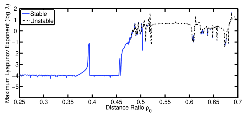
Figure 1: Maximum Lyapunov exponent is plotted versus the distance ratio $\rho_{0}$ for $\mu=0.1$. The stable and unstable cases are denoted.

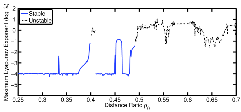
Figure 2: Same as Fig. 1 but for $\mu=0.2$.

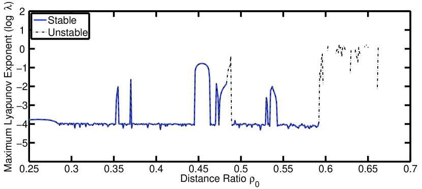
Figure 3: Same as Fig. 1 but for $\mu=0.3$.

In order to determine resonances, we utilize the method of Lyapunov exponents (e.g., Nesvorný & Morbidelli 1998; Nesvorný et al. 2002). In this method, we consider a constant mass ratio $\mu$, calculate the spectrum of Lyapunov exponents, and monitor the maximum Lyapunov exponent with respect to the parameter $\rho_{0}$. Although we calculate the full spectrum of Lyapunov exponents, we limit this discussion to the maximum Lyapunov exponent for the reasons explained elsewhere (e.g., Quarles et al. 2011). The maximum Lyapunov exponent is used as an indicator of the maximum role that a particular resonance will have on the system. This provides us with a way of inspecting how the maximum Lyapunov exponent changes in response to small variations in the initial condition $\rho_{0}$. Additionally, we use the fast Lyapunov indicator (e.g., Froeschlé, Gonczi & Lega 1997; Lega & Froeschlé 2001) to estimate the extent of weak chaotic or ordered motion.

After choosing a value of $\mu$ and performing calculations of the maximum Lyapunov exponent, we use a FFT to produce a periodogram, and then take ratios of the periods in the periodogram to determine what kind of resonances (if any) are present. Using the Lyapunov exponent with a periodogram provides a method of quickly identifying regions of possible resonances rather than invoking a brute force method of performing a FFT over all possible values of $\rho_{0}$. The ratios of the periods in the periodogram are taken with respect to the period axis; however, the strength of the peaks are not considered. In the tables, we provide the periods of the three strongest peaks in the periodogram and label them as Peak 1, Peak 2, and Peak 3 in ascending order. Resonance 1 denotes the closest rational expression of the ratio of Peak 2 to Peak 1, whereas Resonance 2 denotes the closest rational expression of Peak 3 to Peak 1. More peaks may be possible in the periodograms; however, the induced instability greatly overwhelms the necessity for investigating them. There are also elements in the tables without data (shown by ellipsis). They indicate simulations where a Peak 3 could not be discriminated against the background; therefore, a value for Resonance 2 could not be determined. We study the range of $\rho_{0}$ beginning at $\rho_{0}=0.250$ and ending at $\rho_{0}=0.700$ in increments of $0.001$ for a given value of $\mu$.

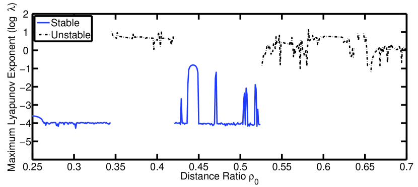
Figure 4: Same as Fig. 1 but for $\mu=0.4$.

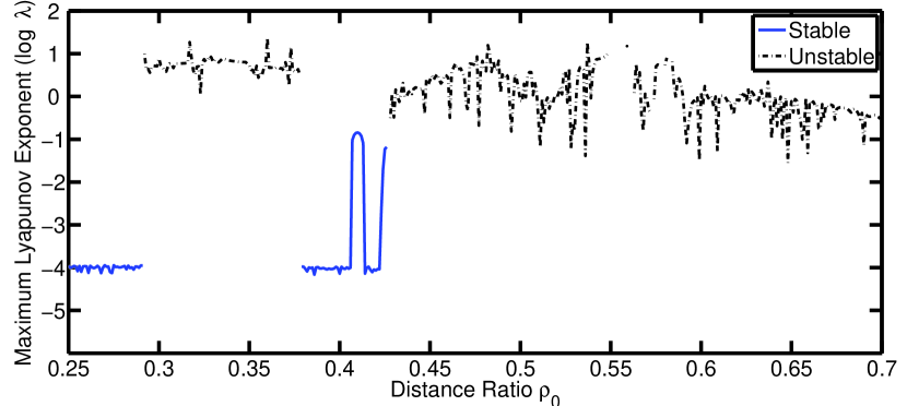
Figure 5: Same as Fig. 1 but for $\mu=0.5$.

Table 1: Resonances for selected values of $\rho_{0}$ with an elevated maximum Lyapunov exponent given for $\mu=0.1$. The different orbital types are classified as Periodic, Quasi-Periodic, and Non-Periodic, and are denoted by P, QP, and NP, respectively.

$\rho_{0}$	Peak 1	Peak 2	Peak 3a	Resonance 1	Resonance 2a	Orbital Type
0.394	0.3494	1.045	…	3:1	…	P
0.457	0.4693	0.8827	1.001	15:8	17:8	P
0.471	0.4832	0.9671	…	2:1	…	P

• ^aNote: Elements without data indicate simulations that did not have a Peak 3 in the periodogram; therefore, a value for Resonance 2 could not be determined.

Table 2: Same as Table 1 but for $\mu=0.2$.

$\rho_{0}$	Peak 1	Peak 2	Peak 3	Resonance 1	Resonance 2	Orbital Type
0.334	0.2715	1.087	…	4:1	…	P
0.391	0.3631	1.143	…	22:7	…	QP
0.399	0.3756	1.127	…	3:1	…	QP
0.450	0.4636	0.7716	1.162	5:3	5:2	QP
0.458	0.4769	0.815	1.151	12:7	12:5	QP
0.482	0.5153	1.031	…	2:1	…	P
0.491	0.3457	0.5186	1.037	3:2	3:1	QP

Table 3: Same as Table 1 but for $\mu=0.3$.

$\rho_{0}$	Peak 1	Peak 2	Peak 3	Resonance 1	Resonance 2	Orbital Type
0.355	0.3267	1.297	…	4:1	…	QP
0.370	0.3503	1.357	…	31:8	…	QP
0.454	0.4743	1.448	…	3:1	…	QP
0.471	0.4996	1.500	…	3:1	…	P
0.483	0.5121	0.7680	1.537	3:2	3:1	QP
0.488	0.5244	0.8034	1.511	3:2	23:8	NP
0.493	0.5236	0.8278	1.495	14:3	14:5	QP
0.530	0.5906	0.9875	1.472	5:3	5:2	QP
0.537	0.6016	1.017	1.475	5:3	22:9	QP

Table 4: Same as Table 1 but for $\mu=0.4$.

$\rho_{0}$	Peak 1	Peak 2	Peak 3	Resonance 1	Resonance 2	Orbital Type
0.429	0.4456	1.995	…	9:2	…	QP
0.444	0.4726	1.732	…	11:3	…	QP
0.471	0.5236	1.580	…	3:1	…	QP
0.505	0.2958	0.5918	1.480	2:1	5:1	QP
0.507	0.2976	0.5953	1.473	2:1	5:1	QP
0.518	0.2046	0.3070	0.614	3:2	3:1	QP
0.521	0.2060	0.3090	0.618	3:2	3:1	QP

Table 5: Same as Table 1 but for $\mu=0.5$.

$\rho_{0}$	Peak 1	Peak 2	Peak 3	Resonance 1	Resonance 2	Orbital Type
0.410	0.232	0.4639	…	2:1	…	P
0.426	0.251	0.5014	1.506	2:1	6:1	QP

3 Results and Discussion

3.1 Case studies

We consider five different cases of fixed mass ratio $\mu$, starting at $\mu=0.1$ and proceeding in increments of $0.1$. Each case presents a different aspect of the problem but together the combined results allow us to identify and classify resonances in the coplanar CR3BP for relatively large values of $\mu$. For each case, we start with the parameter $\rho_{0}$ at the value $0.250$ that is increased in increments of $0.001$ up to a final value of $\rho_{0}=0.700$. We show one plot and one table for each case of $\mu$. In each plot, we distinguish between the stable cases, which continued for the full $10^{5}$ binary orbits of simulation time by a solid line, and the unstable cases by dashed lines; the latter ended early due to the ejection of the planet from the system. Our criteria for ending each simulation are based on checking the error in the Jacobi constant and the value of the maximum Lyapunov exponent where high values of either imply a high probability for $m_{3}$ to be ejected from the system (Quarles et al. 2011). We also pursued numerical comparisons with an independent integration method to verify the integrity of the proposed outcome (see Section 2). These separate criteria provide us with a method for checking for instability and stability, as well as a measure for identifying chaos in the system. In the accompanying tables, we provide the values of $\rho_{0}$ where the maximum Lyapunov exponent is found to peak.

After the maximum Lyapunov exponent is calculated, we transform the system pointwise from barycentric coordinates to Jacobi coordinates choosing the more massive body as reference point. We perform a FFT using the time series data for that specific $\rho_{0}$. With this result, we obtain the Fourier spectrum and convert it to a corresponding periodogram. The resonances are determined by taking the ratio of periods for the strongest peaks. In the tables, we provide the computational results for the three strongest peaks, if available, for that value of $\rho_{0}$. The resonances are given as a ratio of the period of the small ($m_{3}$) mass to the period of the smaller binary ($m_{2}$) mass. For example, 4:1 would tell us that the small mass orbits four times in a single orbit of the smaller binary mass.

The first case of $\mu=0.1$ is depicted in Fig. 1 with numerical results given in Table 1. This case illustrates a baseline of configurations where the second large ($m_{2}$) mass is not greatly perturbing the small ($m_{3}$) mass from $\rho_{0}=0.250$ to $0.350$. This provides a clear indication of where a possible resonance is not substantial enough to alter the orbit. However, the value of the maximum Lyapunov exponent peaks first at $\rho_{0}=0.394$. This indicates that the second large mass is at a specific geometric position allowing it to greatly perturb the motion of the small mass. The same feature occurs again at $\rho_{0}=0.457$ and $0.471$. Note that the resonances associated with each peak in Fig. 1 are not all the same; see Table 1. Moreover, we identify a large region of instability when $\rho_{0}$ is further increased, which is consistent with previous investigations (Eberle & Cuntz 2010; Quarles et al. 2011).

The second case of $\mu=0.2$ is depicted in Fig. 2 and the relevant numerical values are presented in Table 2. This case differs from the preceding one as now the first resonance peak occurs sooner at $\rho_{0}=0.334$. This is expected because by increasing the value of $\mu$, the perturbing mass has a greater ability to interact with the smaller mass to alter its orbit. There exists a stability region from $\rho_{0}=0.250$ to $0.333$. However, the value of the maximum Lyapunov exponent peaks at seven different values of $\rho_{0}$, which demonstrates the greater influence of the perturbing mass $m_{2}$ compared to the case of $\mu=0.1$. Also, there are apparent gaps surrounding the instability regions. Actually, they are due to our increment size in $\rho_{0}$ and, therefore, these regions should be treated as continuous with appropriate lines transitioning from one region to the next. There is also a resonance plateau in the range of $\rho_{0}=0.45$ to $0.48$. This illustrates a region where the phenomena of resonance is widespread; note there is a similar feature in the study of asteroids (i.e., the 3:1 resonance at 2.5 AU or $\rho_{0}=0.48$).

The third case of $\mu=0.3$ is depicted in Fig. 3 and the associated numerical results are given in Table 3. Here the first resonance peak occurs at $\rho_{0}=0.355$. It also exhibits a well-pronounced region where the resonance is not substantial enough to alter the orbit of the small mass $m_{3}$ as shown in Fig. 3 from $\rho_{0}=0.250$ to $0.354$. The value of the maximum Lyapunov exponent peaks at $9$ different values of $\rho_{0}$ before reaching the stability limit at $\rho_{0}=0.600$ as shown by Eberle et al. (2008). It is important to note that the number of resonance peaks has increased thus far as the value of $\mu$ has increased. Also this case includes a peak in the maximum Lyapunov exponent, where the system is unstable at $\rho_{0}=0.488$ leading to planetary ejection. The transition to this instability is shown by the developing resonances at $\rho_{0}=0.483$ in Table 3.

The fourth case of $\mu=0.4$ is depicted in Fig. 4 with numerical results given in Table 4. This case differs from the preceding trend by the first resonance peak; this peak is delayed and occurs at $\rho_{0}=0.429$ after an instability island. This is due to the perturbing mass gaining an overwhelming amount of gravitational influence over the small mass and creating an instability region from $\rho_{0}=0.350$ to $0.400$. Due to this change there are fewer positions for resonance to occur, the resonances become denser with respect to $\rho_{0}$, and the value of the maximum Lyapunov exponent peaks at $7$ different values of $\rho_{0}$.

The final case of $\mu=0.5$ is depicted in Fig. 5 and the relevant numerical results are given in Table 5. This case differs as the first resonance peak is found to occur sooner at $\rho_{0}=0.410$. The Copenhagen case shows the worst case scenario for the small mass because the tug of war between the large masses becomes the most extreme. As a result there is only two narrow regions of stability. The value of the maximum Lyapunov exponent peaks at only two different values of $\rho_{0}$. The first resonance characterizes a stable resonance, whereas the second is a resonance that shows the transition from stability to instability via resonance overlap.

3.2 Classification of resonances

In Tables 1 to 5, we identified the existence of 2 possible resonances. We now discuss them separately starting with the results obtained for Resonance 1. These results show that the 2:1 resonance occurs in all considered cases of $\mu$, except $\mu=0.3$. It is also shown that the 2:1 resonance is the most common resonance in the coplanar CR3BP in agreement with previous asteroidal investigations. The 3:1 resonance is the second most common resonance as it occurs in all cases except $\mu=0.5$. A new and interesting result is that both the 3:2 and 5:3 resonances occur more often than the 4:1 resonance, which only occurs for $\mu=0.2$ and $0.3$.

The overall picture obtained from the special cases of the values considered for $\mu$ is that the best chance for a resonance occurs at the intermediate value of $\mu=0.3$. In this case, we see that systems start with a resonance reflecting a large ratio of the small mass period to the large mass period. Then as the parameter $\rho_{0}$ increases, so does the value of the ratio. After crossing the smoothest peak at $\rho_{0}=0.454$, the secondary resonances are formed; these resonances are labeled as Resonance 2 in Tables 1 to 5 and once they appear their existence may imply instability caused by resonance overlap. Among these resonances, the 3:1 resonance is the most dominant but new resonances such as 5:2 also occur, which is present for $\mu=0.2$ and $0.3$, and 5:1 occurring for $\mu=0.4$. An interesting result is that only the 3:1 resonance occurs also as a secondary resonance and that none of the other resonances labeled as Resonance 1 also occur as Resonance 2.

Additionally, we can classify resonances based on the behaviour of the orbits. In Tables 1 to 5, we show classifications based on orbit diagrams in rotating coordinates (see Figs. 6 to 9a) and the osculating semimajor axis of the small mass (see Figs. 6 to 9b). The three classes are periodic, quasi-periodic, and non-periodic, denoted by P, QP, and NP, respectively. Periodic orbits are those that are well-defined (i.e., minimal deviation from the path traced by previous orbits). They are closed, show periodic variations in the osculating semimajor axis, and show two dominant peaks in the corresponding periodogram (see Figs. 6c, 7c, and 9c). Quasi-periodic orbits are those that precess or fill an annulus with an inner and outer boundary. Moreover, quasi-periodic orbits exhibit a more complicated osculating semimajor axis as well as a periodogram with several peaks (see Figs. 7b,c). Non-periodic orbits are those that do not show a regular pattern and are thus most likely to be unstable. Also non-periodic cases show the greatest number of peaks in their periodograms. Of the cases presented, a low value of $\mu$ yields a greater probability for periodic orbits. As the mass ratio $\mu$ increases, the probability for quasi-periodic orbits increases due to increasing influence of the perturbative mass and duration of the perturbation. However, there are some periodic orbits that exist for large values of $\mu$. They occur near the smooth plateau that forms in each of the figures.

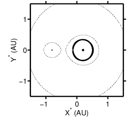
(a)

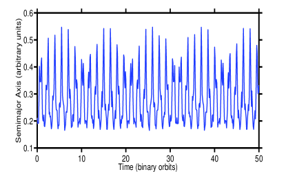
(b)

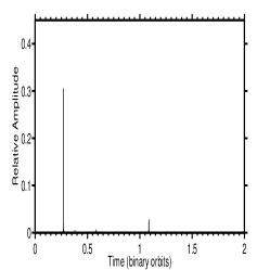
(c)

Figure 6: Case study showing the results for $\mu=0.2$ and $\rho=0.334$. Panel (a) shows the orbit of a planet in a rotating coordinates system, (b) shows the osculating semimajor axis for the first 50 binary orbits, and (c) shows the Fourier periodogram to determine the possible resonances.

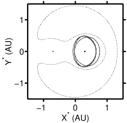
(a)

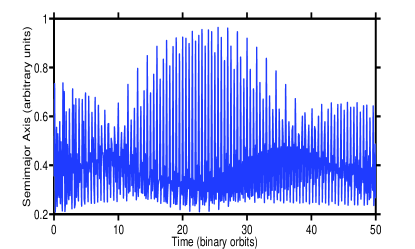
(b)

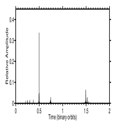
(c)

Figure 7: Case study showing the results for $\mu=0.3$ and $\rho=0.471$. Panel (a) shows the orbit of a planet in a rotating coordinates system, (b) shows the osculating semimajor axis for the first 50 binary orbits, and (c) shows the Fourier periodogram to determine the possible resonances.

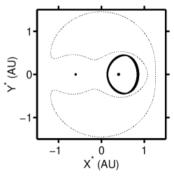
(a)

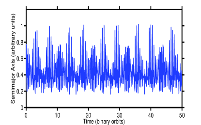
(b)

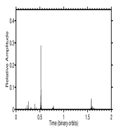
(c)

Figure 8: Case study showing the results for $\mu=0.4$ and $\rho=0.471$. Panel (a) shows the orbit of a planet in a rotating coordinates system, (b) shows the osculating semimajor axis for the first 50 binary orbits, and (c) shows the Fourier periodogram to determine the possible resonances.

(a)

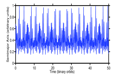
(b)

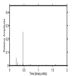
(c)

Figure 9: Case study showing the results for $\mu=0.5$ and $\rho=0.410$. Panel (a) shows the orbit of a planet in a rotating coordinates system, (b) shows the osculating semimajor axis for the first 50 binary orbits, and (c) shows the Fourier periodogram to determine the possible resonances.

4 Summary and conclusions

The case studies of the coplanar CR3BP presented in this paper were used to identify and classify resonances in the coplanar CR3BP. Our method of finding resonances is based on the concept of Lyapunov exponents, or more specifically, it uses the maximum Lyapunov exponent. Based on the latter, we were able to determine where the resonances occurred for a fixed value of mass ratio $\mu$. The conditions for uncovering these resonances were determined by the value of the maximum Lyapunov exponent at the end of each simulation. The fact that the value of the maximum Lyapunov exponent peaks at specific values of distance ratio $\rho_{0}$ provides a strong indicator for the positions of the resonances. Using this method, we have shown that stability is ensured for high values of resonance (i.e., high integer ratios) where only a single resonance is present.

We identified the primary and secondary resonances in the coplanar CR3BP as Resonance 1 and 2 (see Tables 1 to 5), have shown that the 2:1 resonance occurs most frequently as Resonance 1 in the considered systems, and have shown that the 3:1 resonance is the next most common. An interesting result is that there are two other resonances, which are 3:2 and 5:3, and that they occur more often than the 4:1 resonance. Among the resonances labeled as Resonance 2, the 3:1 resonance is the most dominant but there are also new resonances such as 5:2 and 5:1. Moreover, we found that the 3:1 resonance is the only one that also occurs as a secondary resonance, and that none of the other resonances identified by us as Resonance 1 also occur as Resonance 2. The existence of the resonances labeled as Resonance 2 is important as it may imply the onset of instability caused by the resonance overlap.

We also classified the resonances in the coplanar CR3BP based on the behaviour of the orbits. The following three different classes were used: periodic (P), quasi-periodic (QP), and non-periodic (NP); see Eberle & Cuntz (2010) and Quarles et al. (2011) for previous usages of these classes in conjunction with proposed criteria for the onset of orbital instability. Among the considered cases, a low value for $\mu$ and $\rho_{0}$ entailed a greater probability for periodic orbits to occur. Then, the probability for quasi-periodic orbits increases as $\mu$ increases. However, we also discovered some periodic orbits that exist for large values of $\mu$.

The resonances reported in this paper are consistent with the previously established resonances for the Solar System, specifically, in the asteroid belt with its dominant 2:1 resonance (Ferraz-Mello 1994). They used digital filtering and Lyapunov characteristic exponents to determine stochasticity of the eccentricity. This is consistent with our usage of Lyapunov exponents as we took an alternate approach, which is varying the mass ratio instead of the eccentricity. Our approach provides general results for the cases where $\mu$ is considerably greater than the value of $\mu$ in Sun–Jupiter-type systems but where the eccentricity is small. Although our results have been obtained for the special case of the coplanar CR3BP, we expect that it will be possible to augment our findings to planets in general stellar binary systems. Desired generalizations should include studies of the ER3BP (e.g., Pilat-Lohinger & Dvorak 2002; Szenkovits & Makó 2008) as well as applications to planets in previously discovered star–planet systems.