The pulsar force-free magnetosphere linked to its striped wind: time-dependent pseudo-spectral simulations

Abstract

Pulsar activity and its related radiation mechanism are usually explained by invoking some plasma processes occurring inside the magnetosphere, be it polar caps, outer/slot gaps or in the transition region between the quasi-static magnetic dipole regime and the wave zone, like the striped wind. Despite many detailed local investigations, the global electrodynamics around those neutron stars remains poorly described with only little quantitative studies on the largest scales, i.e. of several light-cylinder radii $r_{\rm L}$. Better understanding of these compact objects requires a deep and accurate knowledge of their immediate electromagnetic surrounding within the magnetosphere and its link to the relativistic pulsar wind. This is compulsory to make any reliable predictions about the whole electric circuit, the energy losses, the sites of particle acceleration and the possibly associated emission mechanisms.

The aim of this work is to present accurate solutions to the nearly stationary force-free pulsar magnetosphere and its link to the striped wind, for various spin periods and arbitrary inclination. To this end, the time-dependent Maxwell equations are solved in spherical geometry in the force-free approximation using a vector spherical harmonic expansion of the electromagnetic field. An exact analytical enforcement of the divergenceless of the magnetic part is obtained by a projection method. Special care has been given to design an algorithm able to look deeply into the magnetosphere with physically realistic ratios of stellar $R_{*}$ to light-cylinder $r_{\rm L}$ radius. However, currently available computational resources allows us only to set $R_{*}/r_{\rm L}=10^{-1}$ corresponding to pulsars with period $2$ ms. The spherical geometry permits a proper and mathematically well-posed imposition of self-consistent physical boundary conditions on the stellar crust. We checked our code against several analytical solutions, like the Deutsch vacuum rotator solution and the Michel monopole field. We also retrieve energy losses comparable to the magneto-dipole radiation formula and consistent with previous similar works. Finally, for arbitrary obliquity, we give an expression for the total electric charge of the system. It does not vanish except for the perpendicular rotator. This is due to the often ignored point charge located at the centre of the neutron star. It is questionable if such solutions with huge electric charges could exist in reality except for configurations close to an orthogonal rotator. The charge spread over the stellar crust is not a tunable parameter as is often hypothesized.

1 INTRODUCTION

The problem of energy losses, i.e. particle acceleration and radiation, from an active pulsar is closely related to the electric current circulation within its magnetosphere, the geometry of close and open magnetic field lines, the processes of gap formation and the way the current is closed. It has been argued that this current flows outside the light-cylinder, where very strong dissipation arises and manifests itself as high-energy radiation. Because the electromagnetic field dominates the dynamics at least close to the neutron star surface, low or even vanishing particle inertia and zero pressure is often assumed. This corresponds to a zero-th order approximate solution to the pulsar magnetosphere and refered as relativistic force-free electrodynamics or more properly electromagnetodynamics. Steady axisymmetric magnetospheres have been treated on an analytical basis for charge-separated plasma by Okamoto (1974) and then extended to normal plasma by the same author (Okamoto, 1975). It is well known that the force-free magnetic field in the far zone well outside the light-cylinder should create a current sheet propagating outwards like a vacuum wave (Buckley, 1977). The force-free approximations has been applied to magnetospheres of compact objects, especially to those of pulsars, known as the pulsar equation, for the axisymmetric rotator (Michel, 1973a; Scharlemann & Wagoner, 1973; Endean, 1974) with attempts to solve it numerically (Gruzinov, 2006). An exact analytical solution has been found for the special case of a magnetic monopole (Michel, 1973b). Although not realistic close to the neutron star, it gives some insight into the far field solution, reaching asymptotically a purely radial structure. Many authors investigated the aligned rotator because axisymmetry and time independence lead to some drastic simplifications, although this does not really correspond to a pulsar (Contopoulos et al., 1999; Timokhin, 2006; Komissarov, 2006; McKinney, 2006). Therefore, several authors tried to construct a force-free pulsar magnetosphere by direct time-dependent simulations of Maxwell equations in the general oblique case (Spitkovsky, 2006). Difficulties with outer boundary conditions due to reflection, cured by perfectly matching layers (Kalapotharakos & Contopoulos, 2009) improved this algorithm by implementing some absorbing outer boundary conditions. However, the large ratio between stellar to light-cylinder radius $R_{*}/r_{\rm L}=0.2$ used in these previous works are not realistic for observed pulsar periods (this would correspond to a 1 ms pulsar). Moreover, the system has to reach a stationary state after some relaxation time that needs several rotation periods and which is difficult to control with boundary conditions that are not strictly non-reflecting. However, this force-free approach was recently extended by including resistivity (Li et al., 2012).

Finding analytical or semi-analytical solutions is possible only in a very few cases. For instance, Mestel et al. (1999) solved the equations for the perpendicular rotator without aligned currents. Therefore the linearity of the problem allowed them to employ Fourier techniques for expanding the solution.

However, more realistic models should leave the force-free description. Indeed Kojima & Oogi (2009) presented a two-fluid solution to the aligned rotator. Nevertheless, alternative models with non-neutral fully charged separated magnetospheres containing huge vacuum gaps have also been proposed and known as electrospheric models. The early simulations of Krause-Polstorff & Michel (1985) for the aligned rotator have been improved by Pétri et al. (2002) and extended to oblique rotators (McDonald & Shearer, 2009).

Back to the force-free simulations discussed above, some drawbacks should be pointed out. First, using a Cartesian coordinate system renders it painful to impose proper and convincing inner boundary conditions on the stellar surface, to a good approximation depicted as a perfect sphere. Investigating the polar cap configuration becomes therefore a difficult task. On the outer boundary, reflecting outgoing waves can hardly be avoided as explained. Therefore, relaxation to a stationary state becomes difficult to recognize. Probably the strongest flaw is that the full expression for the force-free current density is not taken into account, the part along the magnetic field line being dropped because of its intricated expression including spatial derivatives, tricky to handle with finite difference schemes. Parfrey et al. (2011) improved the situation by implementing a pseudo-spectral code in spherical geometry for the axisymmetric pulsar magnetosphere. Unfortunately, the code presented in this paper does not strictly, or at least numerically, satisfy the divergenceless of the magnetic field, ${\rm div}\,\mathbf{B}=0$, for instance by an explicit imposition of this condition. Spurious magnetic monopoles could locally be present when evolving Maxwell equations in time. Moreover it seems that regularity conditions at the poles were overlooked and are not ensured. This is probably due to inadequate expansion techniques of a vector field viewed as a set of scalar fields for each of its components.

On a more fundamental side, Uchida (1997a) presented a formalism introducing Euler potential to solve the time-dependent force-free equations with special emphasize to symmetries (Uchida, 1997b). Punsly (2003) studied the waves allowed by the force-free approximation and found that the Alfven and fast modes behave similarly to MHD waves in the limit of vanishing particle inertia.

In this paper, we demonstrate how to overcome many of the aforementioned limitations by a proper and efficient expansion of a general vector field onto vector spherical harmonics, ensuring regularity and smoothness across the poles. We would like to stress that the simulations presented here were performed on a single processor for several hours to days or weeks and relatively modest grids of resolution $N_{r}\times N_{\vartheta}\times N_{\varphi}=257\times 32\times 64$ at most. This is in clear contrast with finite difference simulations employing grids as huge as $1000^{3}$ therefore inevitably requiring parallelization and/or supercomputers. We present full force-free pulsar magnetosphere solutions in nearly stationary state using spherical polar coordinates. The outline of this paper is as follows. The time-dependent force-free model is exposed and compared to a situation where the regime is strictly stationary, §2. The pseudo-spectral method of solution is presented in §3. The code is then tested and validated against exact analytical solutions, §4. Next, the magnetospheric geometry and properties are described in depth in §5, providing the link to the base of the striped wind, region believed to produce the high-energy pulsed emission (Pétri, 2009; Bai & Spitkovsky, 2010; Pétri, 2011). The magnetic topology is presented for an aligned, an oblique, and an orthogonal rotator, energy losses versus obliquity and total electric charge. Conclusions and possible extensions are drawn in §6.

2 THE MODEL

In this section, we briefly recall the time-dependent Maxwell equations in a force-free regime. Next we address the problem of stationary force-free equations for an oblique rotator and demonstrate that the magnetic field is the main unknown from which all other meaningful quantities are immediately computed. Actually the problem is reduced to two kind of scalar fields by a vector spherical harmonic expansion. The equations for the stationary state serve as an a posteriori check for the time-dependent simulations to their closeness to stationarity.

2.1 Time-dependent Maxwell equations

The time-dependent Maxwell equations in a flat space-time read

$$\partial_{t}\mathbf{B} = -\mathrm{\mathbf{rot}}\,\mathbf{E}$$ (1)

$$\partial_{t}\mathbf{E} = c^{2}\,\mathrm{\mathbf{rot}}\,\mathbf{B}-\frac{\mathbf{j}}{\varepsilon_{0}}$$ (2)

supplemented with the two initial conditions

$${\rm div}\,\mathbf{B} = 0$$ (3)

$${\rm div}\,\mathbf{E} = \frac{\rho_{\rm e}}{\varepsilon_{0}}$$ (4)

In a magnetically dominated relativistic flow such as those expected in pulsar magnetospheres, the force-free approximation implies negligible particle inertia as well as negligible thermal pressure. The Lorentz force acting on a plasma fluid element must therefore vanish, i.e.

$$\rho_{\rm e}\,\mathbf{E}+\mathbf{j}\wedge\mathbf{B}=\mathbf{0}$$ (5)

the charge density being deduced from Maxwell-Gauss equation as

$$\rho_{\rm e}\equiv\varepsilon_{0}\,{\rm div}\,\mathbf{E}$$ (6)

This defines the particle density number with respect to the electric field and not conversely. Thus we assume that there is a source of charge if necessary to maintain the force-free electromagnetic field.

From the force-free condition and the set of Maxwell equations, the current density is found to be (Gruzinov, 2006)

$$\mathbf{j}=\rho_{\rm e}\,\frac{\mathbf{E}\wedge\mathbf{B}}{B^{2}}+\frac{\mathbf{B}\cdot\mathrm{\mathbf{rot}}\,\mathbf{B}/\mu_{0}-\varepsilon_{0}\,\mathbf{E}\cdot\mathrm{\mathbf{rot}}\,\mathbf{E}}{B^{2}}\,\mathbf{B}$$ (7)

The first term represents the contribution from convection of charges due to the electric drift, whereas the second contribution represents the current sustained along magnetic field lines. This expression holds only for magnetically dominated flows. Regions where this condition would not be fulfilled could in principle form behind the light-cylinder and should be avoid. It is difficult to design an elliptic solver passing through the critical points of the flow and meanwhile imposing the conditions for the force-free approximation. We tried different iterative algorithms with several prescriptions behind the light-cylinder but did not get highly accurate solutions as we would expect from spectral methods. We therefore decided to switch back to a time dependent formulation of the problem as exposed in the previous lines. These time-dependent Maxwell equations (1) and (2) are integrated with standard explicit schemes as will be explained in section 3.

2.2 Towards the stationary state

It is difficult to decide whether or not the system has reached a steady state at the end of the run. This is especially true for non axisymmetric magnetospheres for which all fields remain time-dependent in the observer frame. It is therefore useful to get a more quantitative criterion for stationary as described in this paragraph. In a quasi-stationary state, the neutron star drags its magnetosphere and its wind into a rigidly corotating body with constant angular speed $\Omega$. Mathematically speaking, this is written as an equivalence between partial time derivative and partial azimuthal derivative such that for any vector field $\mathbf{V}$ (Muslimov & Harding, 2005)

$$\partial_{t}\mathbf{V}=-\Omega\,\partial_{\varphi}\mathbf{V}+\mathbf{\Omega}\wedge\mathbf{V}=\mathrm{\mathbf{rot}}\,(\mathbf{\beta}\wedge\mathbf{V})-\mathbf{\beta}\,{\rm div}\,\mathbf{V}$$ (8)

where we introduced spherical polar coordinates denoted by $(t,r,\vartheta,\varphi)$ and $\mathbf{\beta}=\mathbf{\Omega}\wedge\mathbf{r}$ is the corotation velocity. Note that the partial derivative with respect to $\varphi$

$$\partial_{\varphi}\mathbf{V}=\partial_{\varphi}(V^{r}\,\vec{e}_{\rm r}+V^{\vartheta}\,\vec{e}_{\vartheta}+V^{\varphi}\,\vec{e}_{\varphi})$$ (9)

includes the orthonormal basis decomposition $(\vec{e}_{\rm r},\vec{e}_{\vartheta},\vec{e}_{\varphi})$. Therefore this basis will also suffer some transformations during the differentiation process. This explains the presence of the cross product $\mathbf{\Omega}\wedge\mathbf{V}$ in the second term in the middle part of equation (8). Stated more simply, it means that we only need to take partial derivatives of the components of the vector $\mathbf{V}$ and not of the vector itself (both being different due to the curvilinear coordinate system). Thanks to this stationarity assumption, Maxwell-Ampère equation is integrated into

$$\mathbf{E}=-\mathbf{\beta}\wedge\mathbf{B}-\mathbf{\nabla}\,\Psi$$ (10)

$\Psi$ being the electric potential as measured in the stellar corotating frame. It is well known that force-free electrodynamics does not allow particle acceleration along magnetic field lines because $\mathbf{E}\cdot\mathbf{B}=\mathbf{B}\cdot\mathbf{\nabla}\,\Psi=0$. This also implies that magnetic field lines are equipotentials for $\Psi$. Moreover, recalling that in the stellar interior, assumed to be a perfect conductor, we have

$$\mathbf{E}=-\mathbf{\beta}\wedge\mathbf{B}$$ (11)

implying $\mathbf{\nabla}\,\Psi=\mathbf{0}$. If there is no gap within the magnetosphere, this assertion must hold in whole space. Therefore Eq. (11) remains valid everywhere, in the neutron star as well as in its magnetosphere. As a consequence, the electric field is just an unessential auxiliary unknown. More importantly, this expression for the electric field automatically satisfies the force-free regime, i.e. $\mathbf{E}\cdot\mathbf{B}=0$. Moreover this implies that at least within the light-cylinder, the flow remains magnetically dominated i.e. $E<c\,B$. To avoid unphysical solutions it is compulsory to add a significant toroidal component of the magnetic field outside the light-cylinder in order to reduce the electric drift speed. Nothing forbids us to extend the investigation well behind the light-cylinder but we were not able so far to find an efficient and self-consistent way to enforce this condition $E<c\,B$ for the boundary value problem implied by the stationary magnetosphere equations. On a more physical ground, in this region, we must either introduce an effective dissipation mechanism or allow for particle acceleration, abandoning the force-free assumption. A numerical trick to enforce magnetically dominated flows everywhere consists to reset the electric field to values less than $c\,B$ in appropriate regions. We are then naturally led to a kind of relaxation process that can be efficiently cast into a time-dependent problem. The algorithm would therefore be very similar to the true time-dependent Maxwell equations so we decided eventually to switch back to time-dependent simulations of the magnetosphere.

It is readily seen that the charge density Eq.(6), the current density, Eq.(7) and the electric field Eq.(11) are all derived from the magnetic field structure. The latter is the only relevant unknown in a stationary force-free problem.

In order to investigate the closeness of the time-dependent solution to a stationary state, we check a posteriori that $\mathbf{E}\approx-\mathbf{\beta}\wedge\mathbf{B}$. Moreover, the stationary Maxwell-Ampère equation reads

$$\mathrm{\mathbf{rot}}\,\mathbf{B}=\mu_{0}\,\mathbf{j}-\frac{\Omega}{c^{2}}\,\partial_{\varphi}\mathbf{E}+\frac{\mathbf{\Omega}}{c^{2}}\wedge\mathbf{E}$$ (12)

which furnishes the second criterion to check the relevance of relaxation to a stationary state.

3 Numerical algorithm

Finding the structure of the stationary pulsar magnetosphere is equivalent to relaxing the time-dependent Maxwell equations towards a stationary state with vanishing partial time derivatives $\partial_{t}\mathbf{E}=\partial_{t}\mathbf{B}=0$ in the corotating frame or satisfying Eq.(8) in the lab frame. To this end, we developed a pseudo-spectral collocation method in space to compute spatial derivatives and augmented by a standard explicit in time ODE integration scheme. The real strength of our code is the use of spherical geometry without coordinate singularity along the polar axis and proper boundary conditions on the stellar surface thanks to the vector spherical harmonic expansion exposed in many details in the appendix A. Regularity and smoothness conditions are also automatically satisfied by the vector fields.

3.1 Vector expansion

A clever expansion of these vector fields is the heart of the code. Indeed, electric and magnetic fields are expanded into vector spherical harmonics (VSH) according to

$$\mathbf{E} = \sum_{l=0}^{\infty}\sum_{m=-l}^{l}\left(E^{r}_{lm}\mathbf{Y}_{lm}+E^{(1)}_{lm}\mathbf{\Psi}_{lm}+E^{(2)}_{lm}\mathbf{\Phi}_{lm}\right)$$ (13)

$$\mathbf{B} = \sum_{l=0}^{\infty}\sum_{m=-l}^{l}\left(B^{r}_{lm}\mathbf{Y}_{lm}+B^{(1)}_{lm}\mathbf{\Psi}_{lm}+B^{(2)}_{lm}\mathbf{\Phi}_{lm}\right)$$ (14)

Note that the series expansions contain a finite number of terms, each of them being smooth. As a consequence, the associated vector fields will also remain smooth in the whole computational domain. By definition, it is impossible to rigorously catch a discontinuity with spectral methods. The best we can do is to introduce artificially a transition layer of negligible thickness. From the expansion coefficients, the linear differential operators like ${\rm div}\,$ and $\mathrm{\mathbf{rot}}\,$ can be easily computed in the coefficient space and then inverted back to real space.

It is a special case of spectral methods, known to possess intrinsically very low numerical dissipation and able to resolve sharp boundary layers (Boyd, 2001). However, if discontinuities arise in the solution, due to the Gibbs phenomenon, the convergence rate is drastically altered. This is cured by applying some filtering process to avoid aliasing and to smear the solution, which is equivalent to some very low dissipation and known as super spectral viscosity (Ma, 1998). Various kind of filters can be used as described for instance in Canuto et al. (2006).

Compared to previous works, our approach has severals advantages. First, because the expression for the current density is quite intricated, the field aligned component is usually dropped and replaced by a prescription for dissipation. Here we implement the full expression, convection and field aligned contribution, reducing numerical dissipation to the lowest possible value. Second, outgoing wave boundary conditions are handled exactly by a characteristic compatibility method. Third, inner boundary conditions are prescribed on the stellar surface, i.e on a sphere. We impose continuous electric field components $\{E_{\vartheta},E_{\varphi}\}$ as well as a continuous $B_{r}$ component. Thus the system is well posed and reduces to Deutsch solution for a magnetosphere without current. We now give some details about the algorithm.

3.2 Maintaining the force-free requirements and the divergenceless of $\mathbf{B}$

During the time evolution of the electromagnetic field, the force-free conditions will be violated soon or later. It is therefore necessary to reinforce the $\mathbf{E}\cdot\mathbf{B}=0$ and $E<c\,B$ conditions regularly. Consequently, at each time step, in a first stage, we subtract the magnetic field aligned electric field component by adjusting the new electric field $\mathbf{E}^{\prime}$ such that

$$\mathbf{E}^{\prime}=\mathbf{E}-\frac{\mathbf{E}\cdot\mathbf{B}}{B^{2}}\,\mathbf{B}$$ (15)

This new electric field need not satisfy the requirement $E^{\prime}<c\,B$. In a second stage, we therefore reduce the electric field $\mathbf{E}^{\prime}$ by a factor $E^{\prime}/c\,B$ to finally get the corrected electric field as

$$\mathbf{E}_{\rm cor}=\mathbf{E}^{\prime}\,\sqrt{\frac{c^{2}\,B^{2}}{E^{\prime 2}}}$$ (16)

The electric field is updated with this corrected value where necessary. Next, to insure a divergenceless magnetic field, at each time step, we project the vector $\mathbf{B}$ onto the subspace defined by ${\rm div}\,\mathbf{B}=0$ simply by applying a forward transform to the coefficients $\{f^{B}_{lm}(r,t),g^{B}_{lm}(r,t)\}$ according to Eq. (63) followed by a backward transform to the vector field $\mathbf{B}$, which is analytically divergenceless by definition. This procedure removes the longitudinal part of the magnetic field.

3.3 Exact boundary conditions

The spherical geometry of our code allows an exact enforcement of the boundary conditions on the star. Moreover, (pseudo)-spectral methods reflect perfectly the underlying analytical problem and therefore only requires the same boundary conditions as the original mathematical problem. There is no need for extra boundary conditions as would be the case for finite difference methods. This would make the problem ill-posed and the code unstable. Finite difference algorithms being much more dissipative, they will damp these unstable solutions!

The correct jump conditions at the inner boundary are, continuity of the normal component of the magnetic field $B_{r}$ and continuity of the tangential component of the electric field $\{E_{\vartheta},E_{\varphi}\}$. Explicitly, we have

$$B_{r}(t,R_{1},\vartheta,\varphi) = B_{r}^{0}(t,\vartheta,\varphi)$$ (17)

$$E_{\vartheta}(t,R_{1},\vartheta,\varphi) = -R_{1}\,\Omega\,\sin\vartheta\,B_{r}^{0}(t,\vartheta,\varphi)$$ (18)

$$E_{\varphi}(t,R_{1},\vartheta,\varphi) = 0$$ (19)

Note that the continuity of $B_{r}$ supplemented with the condition Eq. (11) automatically implies the right boundary treatment of the electric field. $B_{r}^{0}(t,\vartheta,\varphi)$ represents the possibly time-dependent radial magnetic field imposed by the star (monopole, split monopole, aligned or oblique dipole).

As a corollary of these boundary conditions, it is impossible and even not self-consistent to force the surface charge density to vanish on the neutron star crust. This quantity will be derived a posteriori from the results of the simulations.

The outer boundary conditions are more subtle to handle. Ideally, we would like outgoing wave conditions in order to prevent reflection from the artificial outer boundary. The appropriate technique is called Characteristic Compatibility Method (CCM) and described in Canuto et al. (2007). We have implemented this technique in spherical geometry. Indeed, the exact radially propagating characteristics are known and given by

$$E_{\vartheta}\pm c\,B_{\varphi} E_{\varphi}\pm c\,B_{\vartheta}$$ ; (20)

within an unimportant factor $r$. In order to forbid ingoing wave we ensure

$$E_{\vartheta}-c\,B_{\varphi} = 0$$ (21)

$$E_{\varphi}+c\,B_{\vartheta} = 0$$ (22)

whereas the other two characteristics are found by

$$E_{\vartheta}+c\,B_{\varphi} = E_{\vartheta}^{\rm PDE}+c\,B_{\varphi}^{\rm PDE}$$ (23)

$$E_{\varphi}-c\,B_{\vartheta} = E_{\varphi}^{\rm PDE}-c\,B_{\vartheta}^{\rm PDE}$$ (24)

the superscript ^PDE denoting the values of the electromagnetic field obtained by straightforward time advancing without care of any boundary condition. The new corrected values are deduced from Eq. (21)-(24). We expect to reach stationarity in the whole computational domain within a reasonable time span.

3.4 Dealiasing and filtering

The source term of Maxwell equations represented by the force-free current density Eq. (7) introduces a strong non-linearity in the problem and therefore aliasing effect for unresolved spatial scales. In principle, the numerator being a cubic product of unknown functions could be cured by zero-padding techniques (Canuto et al., 2006), but the denominator renders this task impossible. Dealiasing of a quotient of two functions can efficiently be achieved by inverting a linear system for one dimensional problem (Debusschere et al., 2005). Unfortunately, this is intractable for our three-dimensional spherical problem. We prefer to use filtering by smoothing the electromagnetic field at each time step after reinforcing the force-free conditions. We use an eighth order exponential filter in all directions with

$$\sigma(\eta)=\textrm{e}^{-\alpha\,\eta^{\beta}}$$ (25)

$\eta$ ranges between 0 and 1. For instance, in the radial coordinate $\eta=k/(N_{r}-1)$ for $k\in[0..N_{r}-1]$, $k$ being the index of the coefficient $c_{k}$ in the Chebyshev expansion $f(x)=\sum_{k=0}^{N_{r}-1}c_{k}\,T_{k}(x)$. We tried several parameter sets, a good compromise between accuracy and stability is $\alpha=10$ and $\beta=8$.

3.5 Time integration

Pseudo-spectral methods aim at replacing a set of partial differential equations (PDE) by a set of ordinary differential equations (ODE) for the unknown collocation points or spectral coefficients. Schematically, we write it as

$$\frac{d\mathbf{u}}{dt}=f(t,\mathbf{u})$$ (26)

with appropriate initial and boundary conditions. $\mathbf{u}$ represents the vector of unknown functions either evaluated at the collocation points or simply the spectral coefficients.

Several methods for integrating the time evolution of those ODE are at hand. It is worth mentioning implicit versus explicit schemes and single versus multi-step marching methods. Runge-Kutta schemes remain very popular as a single step scheme, but their main flaw is the evaluation of the RHS very often. For spectral methods, Adam-Bashforth (explicit scheme) and Adam-Moulton (implicit scheme), known as multi-step integrators, are also widely employed. Their advantage is that no extra cost is needed to compute the right hand side.

Although many time marching algorithms could be justified, we decided to use a third order Adam-Bashforth scheme advancing a vector of unknown functions $\mathbf{u}$ as

$$\mathbf{u}^{n+1}=\mathbf{u}^{n}+\Delta t\,\left(\frac{23}{12}\mathbf{f}^{n}-\frac{16}{12}\mathbf{f}^{n-1}+\frac{5}{12}\mathbf{f}^{n-2}\right)$$ (27)

where $\Delta t$ is the fixed time step subject to some stability restrictions, $\mathbf{u}^{n}=\mathbf{u}(n\,\Delta t)$ and $\mathbf{f}^{n}=\mathbf{f}(n\,\Delta t,\mathbf{u}(n\,\Delta t))$.

Let us say a few words about the time step restriction. For the time-marching scheme to remain stable, $\Delta t$ should remain in the stability region defined by the inequality $v_{\rm max}\,\Delta t\leq\alpha\,\Delta x_{\rm min}$ where $v_{\rm max}$ is the maximum speed of the waves, here equal to the speed of light $c$, $\alpha$ a constant close to unity depending on the integration scheme and $\Delta x_{\rm min}$ the minimum grid spacing between two points. In our spherical computation domain, the severe constraint comes from the inner part because

$$\Delta x_{\rm min}=\textrm{Min}(\Delta r,r\,\Delta\vartheta,r\,\sin\vartheta\,\Delta\varphi)$$ (28)

It is usually claimed that the non-uniform grid introduced by the Chebyshev collocation points, which are very dense at the boundaries, are the most critical conditions because $\Delta r=O(N_{r}^{-2})$. While this is true for Cartesian coordinates, we find actually that the grid spacing along the polar axis imposes an even stronger limit on the time step because of the presence of the factor $r\,\sin\vartheta$ in front of $\Delta\varphi$, depending on the resolution adopted in the radial and transverse directions. This explains why we do not tried a mapping of the Chebyshev collocation points by the popular Kosloff/Tal-Ezer grid (Kosloff & Tal-Ezer, 1993). Such mapping unfortunately kills the spectral convergence properties of the methods, degrading it only to a second order scheme (Boyd, 2001).

4 TEST

Before handling the general oblique rotator, we check our algorithm against some well known analytical solutions. The starting point is the Deutsch vacuum field solution for a perpendicular rotator. Then, we investigate the monopole solutions with a central monopole magnetic field.

In the remaining of the paper, we adopt the following normalization: the magnetic field strength at the light cylinder in the equatorial plane is set to unity, $B_{\rm L}=1$, as well as the stellar angular velocity and the speed of light $\Omega=c=1$, therefore $r_{\rm L}=1$.

4.1 The Deutsch solution

The vacuum electromagnetic field of an oblique rotator is known analytically since the work by Deutsch (1955). Because Maxwell equations are linear in vacuum space, solutions are found through complex analysis. Assuming a star of radius $R_{*}$ and surface magnetic field of $B_{*}$ with rotation speed $\Omega_{*}$ and obliquity $\chi$, the complex electromagnetic field is easily computed and given in the appendix B.

We start the simulation with the perpendicular static dipole magnetic field ($\chi=90\degr$) and zero electric field outside the star, except for the crust where we enforce the inner boundary condition with corotating electric field, see Sec. 3. We performed simulations with different radial extensions of the computational domain and tried several resolutions. For the largest radial dimensions, finer grids in radius are required, therefore increasing the number of radial collocation points  $N_{r}$. Typically, for a domain $r\in[0.2,2]$, a resolution of $N_{r}\times N_{\vartheta}\times N_{\varphi}=33\times 16\times 32$ is sufficient to get accurate solutions. For the largest runs with $r\in[0.1,10]$ we found that a minimum resolution of $N_{r}\times N_{\vartheta}\times N_{\varphi}=257\times 16\times 32$ was necessary.

We let the system evolve for two rotational period of the pulsar. The final magnetic field line configuration in the equatorial plane is shown as dashed blues curves in fig. 1 and compared to the analytical solution depicted as solid red curves. The numerical solution is very close to the exact solution everywhere, they are hardly distinguishable. The associated Poynting flux is shown in fig. 2. It is constant and equal to the Deutsch value everywhere except close to the star. Nevertheless after a thin boundary layer, the flux relaxes sharply to the exact stationary value of Deutsch. In the outer parts of the domain, the system evolved to a nearly steady state configuration and no significant reflections have to be reported. The Poynting flux is normalized to the monopole solution flux, see Eq. (32). It is a bit less than unity because it depends on the ratio $R_{*}/r_{\rm L}$ and tends to Eq. (32) when $R_{*}/r_{\rm L}$ tends to zero.

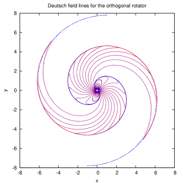
Figure 1: Magnetic field lines of the perpendicular Deutsch field in the equatorial plane. The exact analytical solution (solid red lines) is compared to the time-dependent simulation (dashed blue lines). The overlapping is excellent in the whole region where the relaxation to a quasi-stationary state is nearly achieved.

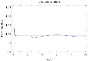
Figure 2: Poynting flux across the sphere of radius $r$. The computed flux (blue line) is almost constant and equal to its analytical value (red line). The solution settled down to the stationary Deutsch field even close to the outer boundary.

This first test demonstrates the ability of our code to handle non axisymmetric configuration with high accuracy and to relax the system to an almost stationary state in a vacuum region.

4.2 The monopole solution

Next we tackle the problem of an axisymmetric force-free flow known as the monopole field introduced by Michel (1973b). We recall that this monopole solution is given by

$$\mathbf{B}=B_{\rm L}\,\frac{r_{\rm L}^{2}}{r^{2}}\,\vec{e}_{\rm r}-B_{\rm L}\,\frac{r_{\rm L}}{r}\,\sin\vartheta\,\vec{e}_{\varphi}$$ (29)

In terms of a vector spherical harmonic (VSH) expansion, this magnetic field is expressed as

$$\mathbf{B}=B_{\rm L}\,\frac{r_{\rm L}^{2}}{r^{2}}\,\vec{e}_{\rm r}+g_{10}^{B}(r)\,\mathbf{\Phi}_{10}$$ (30)

where

$$g_{10}^{B}(r)=\sqrt{\frac{8\pi}{3}}\,B_{L}\,\frac{r_{\rm L}}{r}$$ (31)

all other coefficients being equal to zero. See the appendix A for a detailed exposure of the VSH, their definition and useful properties.

The run is started with a pure monopolar magnetic field and zero electric field outside the star, as before. An Alfven wave is launched from the stellar surface and quickly forces the system to a stationary state. Here also, as expected, larger radial extension implies finer grid in radius. Typically, for a domain $r\in[0.2,2]$, a resolution of $N_{r}\times N_{\vartheta}\times N_{\varphi}=33\times 16\times 32$ is sufficient to get accurate solutions. For the largest runs with $r\in[0.1,10]$ we found that a minimum resolution of $N_{r}\times N_{\vartheta}\times N_{\varphi}=257\times 16\times 32$ was necessary. The relevant coefficient $g^{B}_{10}(r)$ is shown in fig. 3 for comparison with the analytical solution. The numerical solution is very close to the exact solution in the whole computational box. The associated Poynting flux, normalized to the exact monopole value of

$$L_{\rm mono}=\frac{8\,\pi}{3\,\mu_{0}\,c^{3}}\,\Omega_{*}^{4}\,B_{*}^{2}\,R_{*}^{6}=\frac{8\,\pi}{3\,\mu_{0}\,c^{3}}\,\Omega_{*}^{4}\,B_{\rm L}^{2}\,r_{\rm L}^{6}$$ (32)

is depicted in fig. 4. It is almost constant and equal to the monopole value as expected. Note that there is no spurious reflection in the outer regions, we are very close to a steady state configuration.

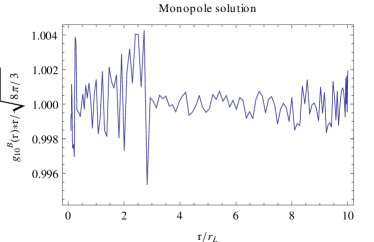
Figure 3: The relevant VSH coefficient $g^{B}_{10}(r)$ for the monopole magnetic field expansion in the domain $r/r_{\rm L}\in[0.1,10]$. For ease to compare, we applied a normalization factor of $r/\sqrt{8\pi/3}$. All other coefficients $g^{B}_{lm}(r)$ with the same normalization factor are less than $10^{-6}$. Results are shown for a resolution of $N_{r}\times N_{\vartheta}\times N_{\varphi}=257\times 16\times 32$.

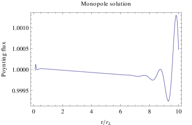
Figure 4: Poynting flux across the simulation sphere corresponding to the numerical solution of fig. 3. It is approximately constant as expected from energy conservation arguments. The same resolution as in fig. 3 applies.

We tried higher resolutions for instance $N_{r}\times N_{\vartheta}\times N_{\varphi}=257\times 32\times 64$ without significant improvement of the computed solutions. All spatial scales have been resolved with the coarsest grid. That such a low resolution is sufficient is no surprise because the monopole solution does only contain two coefficients: the monopole radial part $f^{B}_{00}(r)=B_{\rm L}\,r_{\rm L}^{2}/r^{2}$ and the toroidal part $g^{B}_{10}(r)$, so there exist at most one mode $l=1$.

5 RESULTS

We next look at the oblique pulsar magnetosphere, especially the aligned rotator, studied several times in the past by several authors. New results about the perpendicular rotator and its link to the striped wind will also be shown.

5.1 Simulation setup

The rotating neutron star has a radius$~{}R_{1}$. The computational domain extends from this inner boundary $R_{1}$ to an outer boundary shell of radius $R_{2}>R_{1}$. Note that the star does not belong to the simulation box except for its surface in order to fix the inner boundary conditions. For concreteness, we start from $R_{1}=0.2\,r_{\rm L}$ corresponding to a 1 ms pulsar down to $R=0.1\,r_{\rm L}$ describing a 2 ms pulsar. Likewise the extension of the simulation sphere is variable and equal to $R_{2}=2\,r_{\rm L}$ up to $R_{2}=10\,r_{\rm L}$ to investigate the beginning of the striped wind. The inclination angle of the magnetic moment with respect to the rotation axis was set to $\chi=\{0\degr,30\degr,60\degr,90\degr\}$.

We performed several simulation sets with different filters, the most common being Cesaro, raised cosinus and 2nd, 4th, 8th-order exponential filter (see Canuto et al. (2006)) as well as different spatial resolutions. We found that for spatially resolved discretization, the algorithm converges quickly to a stationary state. We emphasize that the solutions become independent of the choice of a filter as it should be, given us confidence about the convergence and reliability of our results.

5.2 Magnetospheric structure

First, let us have a look on the magnetic field geometry. Let us start with the special case of an aligned rotator. The 3D magnetic field lines are shown in fig. 5. The inner boundary is at $R_{1}=0.2\,r_{\rm L}$ and the outer boundary at $R_{2}=2\,r_{\rm L}$. Inside the light-cylinder, the geometry is close to the static dipole without significant toroidal magnetic field component. Along the polar caps and outside the light-cylinder, we recognize a monopole structure with a significant toroidal component. The aligned rotator, although being simple because axisymmetric and therefore more tractable analytically and computationally, is of no relevance for pulsar theory because it is not able to reproduce the pulsar phenomenon. Inclined models are true pulsars.

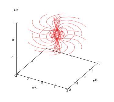
Figure 5: 3D magnetic field lines for the aligned rotator. The inner and outer spherical boundaries are located respectively at $R_{1}=0.2\,r_{\rm L}$ and $R_{2}=2\,r_{\rm L}$.

Thus, we give an example of oblique rotator as shown in fig. 6 with $\chi=60\degr$. The weakly disturbed static dipole regime inside the light-cylinder contrasts with the open field lines passing through the light-cylinder as is costumary for the force-free magnetosphere. Visualization and exploiting data is cumbersome for the full 3D geometry, so we do not discuss further this peculiar case. The orthogonal rotator with its inherent symmetry about the equatorial plane represents the best configuration to study a realistic pulsar magnetosphere.

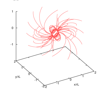
Figure 6: 3D magnetic field lines for the inclined rotator with $\chi=60\degr$. The inner and outer spherical boundaries are located respectively at $R_{1}=0.2\,r_{\rm L}$ and $R_{2}=2\,r_{\rm L}$.

We show such rotator for which vizualisation is easier because some field lines are entirely contained in the equatorial plane. These lines are shown in fig. 7. The inner boundary is at $R_{1}=0.2\,r_{\rm L}$ and the outer boundary at $R_{2}=5\,r_{\rm L}$. The magnetic topology is reminiscent of the Deutsch field solution with some regions of strong deviation due to the magnetospheric current. Inside the light-cylinder (black circle), the geometry is close to the static dipole whereas outside, the launch of the striped wind is seen with its spiral structure in regions of strong magnetic field gradient.

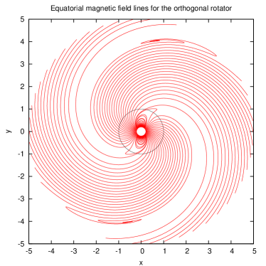
Figure 7: Equatorial magnetic field lines for the perpendicular rotator. The light cylinder is shown as a black circle. The inner and outer spherical boundaries are located respectively at $R_{1}=0.2\,r_{\rm L}$ and $R_{2}=5\,r_{\rm L}$.

In order to compare the orthogonal force-free field with the vacuum field, we did a large scale simulation with $R_{1}=0.1\,r_{\rm L}$ and $R_{2}=10\,r_{\rm L}$ and shown in fig. 8. The shape of the spiral current sheet in the force-free striped wind follows a geometric shape reminiscent to the Deutsch solution. The locus of the current sheet in the striped wind according to the rotational phase of the neutron star has strong implications on the association between radio and high energy emission. The time lag between the radio pulses and the gamma-ray pulses are direct observational consequences and can be checked (Pétri, 2011).

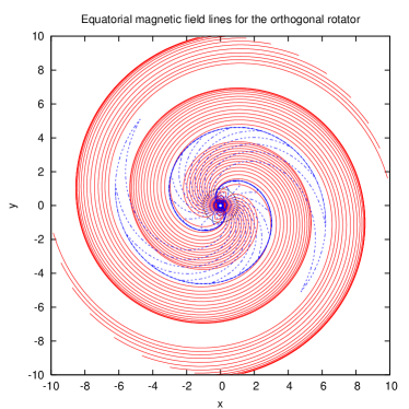
Figure 8: Equatorial magnetic field lines for the perpendicular force-free rotator (red solid line), compared to the vacuum Deutsch field (dashed blue line). The light cylinder is shown as a black circle. The inner and outer spherical boundaries are located respectively at $R_{1}=0.1\,r_{\rm L}$ and $R_{2}=10\,r_{\rm L}$. Note the similarity between both structures.

Inspecting the Poynting flux dependence with respect to radius, fig. 9, we observed a tendency to dissipate the electromagnetic flux well outside the light-cylinder. The employed resolution should still be increased but must wait more computational power.

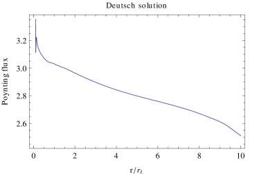
Figure 9: The Poynting flux across the whole simulation sphere for the orthogonal rotator of fig. 8. The Poynting flux is nearly constant but artificial viscosity due to filtering slightly alters energy conservation outside the light-cylinder.

5.3 Energy losses and electric charge

Another important issue is the spin-down energy of the pulsar by magnetic braking. Thanks to the knowledge of the magnetospheric structure, we can investigate the energetics of the pulsar quantitatively. Current wisdom assumes that the Poynting flux escaping from the force-free magnetosphere is of the same order of magnitude as the vacuum dipole rotator. We check this assertion by plotting the Poynting flux across the simulation sphere as a function of the obliquity with a simulation sphere extending from $R_{1}=0.2r_{\rm L}$ to $R_{2}=2r_{\rm L}$, fig. 10, normalized with respect to the magneto-dipole losses for an orthogonal rotator expressed as

$$L_{\rm dip}=\frac{8\,\pi}{3}\,\frac{\Omega^{4}\,B^{2}\,R^{6}}{\mu_{0}\,c^{3}}.$$ (33)

Within a factor of several unity, the luminosity is the same for vacuum dipole and force-free magnetosphere, fig. 10. The flux across the light-cylinder, i.e. before artificial viscosity due to filtering becomes significant can approximately be fitted with, fig. 11,

$$L_{\rm sp}\approx 1.5\,L_{\rm dip}\,(1+\sin^{2}\chi)$$ (34)

Thus the orthogonal force-free magnetosphere radiates 3 times more than the vacuum analog whereas the aligned magnetosphere radiates 50% of the vacuum perpendicular rotator. These results agree with the functional form found by Spitkovsky (2006) although we took into account the full expression for the current density. Surprisingly, we found it easier to look for the perpendicular rotator than for the aligned one. Indeed, in the latter case, the current sheet in the equatorial plane is coarsely resolved by our current grid resolution. According to the lower blue curve in fig. 10, non negligible artificial dissipation is present and smears out the discontinuity. On the contrary, the strong displacement current in the former case leads to more gentle current sheet much better described by the coarse grid. Scrutiny of the upper green curve in fig. 10 demonstrates indeed that the Poynting flux remains nearly constant with radius. Energy is conserved to good accuracy as is expected from the force-free evolution equations (Komissarov, 2002). In order to circumvent high dissipation rate, the only efficient remedy would be to increase the grid resolution. Unfortunately, for the moment we are unable to run such high-resolution simulation on our computer. We plan to improve our code by performing some optimizations and by using parallelization techniques.

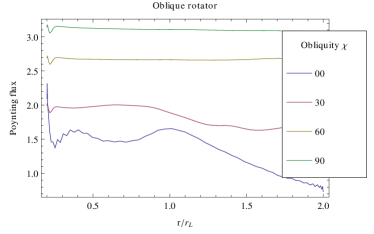
Figure 10: The Poynting flux across the whole simulation sphere as a function of the obliquity $\chi$. The flux is nearly constant for the perpendicular rotator. Artificial dissipation due to filtering becomes significant for almost aligned rotators outside the light-cylinder.

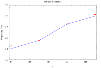
Figure 11: The Poynting flux across the sphere of radius $r_{\rm L}$ as a function of the obliquity $\chi$. Simulation results are depicted by red triangles and the fit is shown in blue solid line.

Finally, the total electric charge enclosed by a spherical shell centered at the pulsar location is computed by the electric flux across it. It is too rarely stated that the total charge of the neutron star and its magnetosphere is not equal to zero but very close to the value of the central point charge $Q_{\rm c}$, located in the middle of the star (see appendix B for the definition of this charge). Indeed, the total charge of the system with respect to obliquity $\chi$ is shown in fig. 12. Only in the special case of an orthogonal rotator is this charge exactly zero. This is true for all ratio $R_{*}/r_{\rm L}$. The fit is simply given by $Q_{\rm ffe}\approx 0.9\,Q_{\rm c}$, fig. 13.

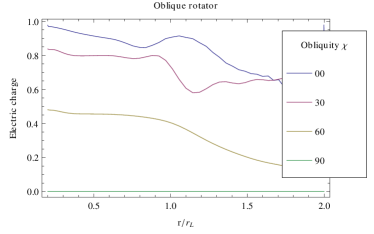
Figure 12: Total electric charge $Q_{\rm tot}$ in the simulation sphere as a function of the obliquity $\chi$ and normalized against the central point charge for the aligned rotator $Q_{\rm c}/\cos\chi$. Simulation parameters are exactly the same as in fig. 10.

Here also, the dependence on $\cos\chi$ is reminiscent of the central point charge $Q_{\rm c}$.

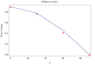
Figure 13: Total electric charge across the sphere of radius $r_{\rm L}$ as a function of the obliquity $\chi$. Simulation results are depicted by red triangles and the fit is shown in blue solid line.

6 CONCLUSION

We solved the full set of time-dependent force-free equations for a rotating oblique pulsar magnetosphere. We tested our pseudo-spectral collocation code and demonstrated that accurate numerical solutions can be found for smooth fields. Interestingly, we found it easier to compute the solution for the perpendicular rotator because the flaw of any spectral method to catch discontinuities is harmless in that particular geometry. It seems that the presence of a strong displacement current facilitates the computation in the vicinity of the current sheet. Unfortunately, the current version of our code does not allow to perform very high resolution on a single processor in a reasonable time to reduce the Gibbs phenomenon for non-smooth configurations as those close to the aligned rotator. We plan to improve the code by optimization and parallelization techniques in the near future. The boundary conditions could certainly also benefit from some more elaborated methods like a sponge layer and non alteration of the boundary value by the filtering process (not yet implemented).

We think that the most physical satisfactory way to get rid of the Gibbs phenomenon related to the thin current sheet would be to alleviate the ideal MHD approximation by including particle inertia. Our code is sufficiently versatile and can be straightforwardly extended to solve the full set of MHD equations. This would bring us closer to reality in the striped structure. Moreover, the magnetic field originates from a compact object of size only twice its Schwarzschild radius. Therefore, we expect not only magnetospheric currents distortion of the magnetic topology, but also general relativistic effects, especially important in the vicinity of the stellar surface and very useful for elucidating the precise geometry of the polar caps. These perturbations due to curved space and dragging of inertial frames, should also be taken into account for an accurate investigation of the emission region close to the magnetic poles.

Appendix A Scalar and vector spherical harmonics

In this appendix, we expose in some details our pseudo-spectral algorithm to compute approximate analytical solutions to the force-free pulsar magnetosphere according to the time-dependent Maxwell equations.

The heart of our scheme resides in the vector spherical harmonic expansion of the two unknown vector fields, the electric and magnetic fields. In the following paragraphs, we discuss in depth the properties of this vector basis. But let us first quickly remind the scalar spherical harmonics.

A.1 Scalar spherical harmonics

The scalar spherical harmonics are defined according to the associated Legendre functions $P_{l}^{m}$ by

$$Y_{lm}(\vartheta) = \sqrt{\frac{2\,l+1}{4\,\pi}\,\frac{(l-m)!}{(l+m)!}}\,P_{l}^{m}(\cos\vartheta)$$ (35)

$$Y_{lm}(\vartheta,\varphi) = Y_{lm}(\vartheta)\,e^{i\,m\,\varphi}$$ (36)

The square root factor imposes normalization of these functions. They are very valuable functions because eigenfunctions of the Laplacian operator in spherical coordinates such that

$$\Delta Y_{lm}(\vartheta,\varphi)=-\frac{l\,(l+1)}{r^{2}}\,Y_{lm}(\vartheta,\varphi)$$ (37)

A useful symmetry property is

$$Y_{l,-m}(\vartheta,\varphi)=(-1)^{m}\,Y_{lm}^{*}(\vartheta,\varphi)$$ (38)

Note that the $Y_{lm}$ form an orthonormal basis on the two-dimensional sphere. Any smooth and regular scalar field can be expanded on this sphere thanks to the spherical harmonics. As explained in the next paragraph, this statement can be generalized to a vector field defined on the sphere.

For completeness, we give the first few $Y_{lm}$ up to $m=3$

$$Y_{00} = \frac{1}{2\sqrt{\pi}}$$

$$Y_{10} = \frac{1}{2}\sqrt{\frac{3}{\pi}}\cos[\vartheta]$$

$$Y_{11} = -\frac{1}{2}e^{i\varphi}\sqrt{\frac{3}{2\pi}}\sin[\vartheta]$$

$$Y_{20} = \frac{1}{4}\sqrt{\frac{5}{\pi}}\left(-1+3\cos[\vartheta]^{2}\right)$$

$$Y_{21} = -\frac{1}{2}e^{i\varphi}\sqrt{\frac{15}{2\pi}}\cos[\vartheta]\sin[\vartheta]$$

$$Y_{22} = \frac{1}{4}e^{2i\varphi}\sqrt{\frac{15}{2\pi}}\sin[\vartheta]^{2}$$

$$Y_{30} = \frac{1}{4}\sqrt{\frac{7}{\pi}}\left(-3\cos[\vartheta]+5\cos[\vartheta]^{3}\right)$$

$$Y_{31} = -\frac{1}{8}e^{i\varphi}\sqrt{\frac{21}{\pi}}\left(-1+5\cos[\vartheta]^{2}\right)\sin[\vartheta]$$

$$Y_{32} = \frac{1}{4}e^{2i\varphi}\sqrt{\frac{105}{2\pi}}\cos[\vartheta]\sin[\vartheta]^{2}$$

$$Y_{33} = -\frac{1}{8}e^{3i\varphi}\sqrt{\frac{35}{\pi}}\sin[\vartheta]^{3}$$

A.2 Vector spherical harmonics

Vector spherical harmonics (VSH) are often used in atomic physics to compute electronic level in atoms. Quantum physicists therefore prefer to work with a normalization of the vectors involving the complex number $i$. Here we adopt a slightly different definition of these vectors by removing this unessential constant factor $i$. More precisely, the three sets of vector spherical harmonics we use are defined by

$$\mathbf{Y}_{lm} = Y_{lm}\,\mathbf{e}_{\rm r}$$ (39)

$$\mathbf{\Psi}_{lm} = \frac{r}{\sqrt{l\,(l+1)}}\,\mathbf{\nabla}Y_{lm}$$ (40)

$$\mathbf{\Phi}_{lm} = \frac{\mathbf{r}}{\sqrt{l\,(l+1)}}\,\wedge\mathbf{\nabla}Y_{lm}$$ (41)

Any smooth three-dimensional vector field $\mathbf{E}$ admits an expansion onto these vectors according to

$$\mathbf{E}(r,\vartheta,\varphi)=\sum_{l=0}^{\infty}\sum_{m=-l}^{l}\left(E^{r}_{lm}(r)\mathbf{Y}_{lm}+E^{(1)}_{lm}(r)\mathbf{\Psi}_{lm}+E^{(2)}_{lm}(r)\mathbf{\Phi}_{lm}\right)$$ (42)

In order to avoid complex numbers, it is sometimes useful to employ instead the trigonometric representation like for instance

$$\mathbf{Y}_{lm}^{c/s} = Y_{lm}(\vartheta)\,\begin{pmatrix}\cos m\,\varphi\\ \sin m\,\varphi\end{pmatrix}\,\mathbf{e}_{\rm r}$$ (43)

and similar expressions for $\{\mathbf{\Psi}_{lm}^{c/s},\mathbf{\Phi}_{lm}^{c/s}\}$.

To link our definition to other authors, note that in quantum mechanics the $\mathbf{\Phi}_{lm}$ are named $\mathbf{X}_{lm}$ and defined by

$$\mathbf{X}_{lm}=\frac{-i}{\sqrt{l\,(l+1)}}\,\mathbf{r}\wedge\mathbf{\nabla}Y_{lm}=-i\,\mathbf{\Phi}_{lm}$$ (44)

A.3 Properties

The vector spherical harmonics share some useful properties with respect to their spatial derivatives. First, assume a 3D scalar field expanded onto the scalar spherical harmonics such that

$$\phi(r,\vartheta,\varphi) = \sum_{l=0}^{\infty}\sum_{m=-l}^{l}\phi_{lm}(r)\,Y_{lm}(\vartheta,\varphi)$$ (45)

Then, its gradient expanded onto the VSH becomes

$$\nabla\phi=\sum_{l=0}^{\infty}\sum_{m=-l}^{l}\left(\frac{\partial\phi_{lm}}{\partial r}\mathbf{Y}_{lm}+\frac{\sqrt{l\,(l+1)}}{r}\,\phi_{lm}\,\mathbf{\Psi}_{lm}\right)$$ (46)

The action of the same gradient on the VSH gives the divergence of any vector field $\mathbf{E}$ as

$$\nabla\cdot\mathbf{E}=\sum_{l=0}^{\infty}\sum_{m=-l}^{l}\left(\frac{1}{r^{2}}\,\frac{\partial}{\partial r}(r^{2}\,E^{r}_{lm})-\frac{\sqrt{l(l+1)}}{r}E^{(1)}_{lm}\right)Y_{lm}$$ (47)

and for the curl

$$\nabla\wedge\mathbf{E} = \sum_{l=0}^{\infty}\sum_{m=-l}^{l}\left[-\frac{\sqrt{l(l+1)}}{r}\,E^{(2)}_{lm}\,\mathbf{Y}_{lm}-\frac{1}{r}\,\frac{\partial}{\partial r}(r\,E^{(2)}_{lm})\mathbf{\Psi}_{lm}+\left(-\frac{\sqrt{l(l+1)}}{r}\,E^{r}_{lm}+\frac{1}{r}\,\frac{\partial}{\partial r}(r\,E^{(1)}_{lm})\right)\,\mathbf{\Phi}_{lm}\right]$$ (48)

For each component taken individually, we find for the divergence

$$\nabla\cdot\left(f(r)\,\mathbf{Y}_{lm}\right) = \frac{1}{r^{2}}\frac{\partial}{\partial r}\left(r^{2}\,f\right)\,Y_{lm}$$ (49)

$$\nabla\cdot\left(f(r)\,\mathbf{\Psi}_{lm}\right) = -\frac{\sqrt{l(l+1)}}{r}\,f\,Y_{lm}$$ (50)

$$\nabla\cdot\left(f(r)\mathbf{\Phi}_{lm}\right) = 0$$ (51)

and for the curl

$$\nabla\times\left(f(r)\,\mathbf{Y}_{lm}\right) =- \frac{\sqrt{l\,(l+1)}}{r}\,f\,\mathbf{\Phi}_{lm}$$ (52)

$$\nabla\times\left(f(r)\mathbf{\Psi}_{lm}\right) = \frac{1}{r}\,\frac{\partial}{\partial r}(r\,f)\mathbf{\Phi}_{lm}$$ (53)

$$\nabla\times\left(f(r)\mathbf{\Phi}_{lm}\right) = -\frac{\sqrt{l(l+1)}}{r}\,f\,\mathbf{Y}_{lm}-\frac{1}{r}\,\frac{\partial}{\partial r}(r\,f)\,\mathbf{\Psi}_{lm}$$ (54)

Finally, define the radial differential operator $\mathcal{D}_{l}$ by

$$\mathcal{D}_{l}=\frac{1}{r^{2}}\,\frac{d}{dr}\left(r^{2}\,\frac{d}{dr}\right)-\frac{l(l+1)}{r^{2}}$$ (55)

The VSH noted $\mathbf{\Phi}_{lm}$ are eigenvectors in the linear algebra meaning, of the vector Laplacian operator $\Delta$. Indeed, it is straightforward to show that

$$\Delta[f(r)\,\mathbf{\Phi}_{lm}]=\mathcal{D}_{l}[f]\,\mathbf{\Phi}_{lm}$$ (56)

It is thus an extension of the properties of the scalar spherical harmonics to the realm of 3D vectors.

A.4 Expansion of a vector field onto VSH

From the above discussion, the components of any vector field can be computed according to the three underlying equalities

$$E_{r} = \sum_{l,m}E_{lm}^{r}\,Y_{lm}$$ (57)

$${\rm div}\,_{\vartheta,\varphi}\vec{E} = \sum_{l,m}-\frac{\sqrt{l(l+1)}}{r}\,E_{lm}^{(1)}\,Y_{lm}$$ (58)

$$\mathrm{\mathbf{rot}}\,\vec{E}\cdot\vec{e}_{\rm r} = \sum_{l,m}-\frac{\sqrt{l(l+1)}}{r}\,E_{lm}^{(2)}\,Y_{lm}$$ (59)

where ${\rm div}\,_{\vartheta,\varphi}\vec{E}$ means taking only the angular part of the divergence. More explicitly, from the definition of the differential operators, we get

$$E_{r} = \sum_{l,m}E_{lm}^{r}\,Y_{lm}$$ (60)

$$\frac{1}{\sin\vartheta}\,\partial_{\vartheta}(\sin\vartheta\,E_{\vartheta})+\frac{1}{\sin\vartheta}\,\partial_{\varphi}\,E_{\varphi} = \sum_{l,m}-\sqrt{l(l+1)}\,E_{lm}^{(1)}\,Y_{lm}$$ (61)

$$\frac{1}{\sin\vartheta}\,\partial_{\vartheta}(\sin\vartheta\,E_{\varphi})-\frac{1}{\sin\vartheta}\,\partial_{\varphi}\,E_{\vartheta} = \sum_{l,m}-\sqrt{l(l+1)}\,E_{lm}^{(2)}\,Y_{lm}$$ (62)

Finding the components of $\mathbf{E}$ is therefore equivalent to finding the expansion coefficients of three scalar fields onto the scalar spherical harmonics. This procedure works for any vector field. However, the magnetic field being divergenceless, only two of the three components are independent. It is therefore judicious to deal properly with those kind of fields by analytically enforcing the condition on the divergence as explained below.

A.5 Expansion of a divergenceless vector field

Any divergenceless vector field is efficiently developed onto the vector spherical harmonic orthonormal basis. This will be the case for the magnetic field in our algorithm.

Assume that the vector field $\mathbf{V}$ is divergenceless. It is helpful to introduce two scalar functions $f_{lm}(r,t)$ and $g_{lm}(r,t)$ such that the decomposition immediately implies the property of divergenceless field. This is achieved by writing

$$\mathbf{V}(r,\vartheta,\varphi,t)=\sum_{l=1}^{\infty}\sum_{m=-l}^{l}\left(\mathrm{\mathbf{rot}}\,[f_{lm}(r,t)\,\mathbf{\Phi}_{lm}]+g_{lm}(r,t)\,\mathbf{\Phi}_{lm}\right)$$ (63)

This expression automatically and analytically enforces the condition ${\rm div}\,\mathbf{V}=0$. Let us quickly draw the way to compute these functions. The transformation from the spherical components to the functions $(f_{lm},g_{lm})$ is given by

$$\mathbf{V}\cdot\vec{e}_{\rm r} = \sum_{l=1}^{\infty}\sum_{m=-l}^{l}-\frac{\sqrt{l\,(l+1)}}{r}\,f_{lm}\,Y_{lm}$$ (64)

$$(\mathrm{\mathbf{rot}}\,\mathbf{V})\cdot\vec{e}_{\rm r} = \sum_{l=1}^{\infty}\sum_{m=-l}^{l}-\frac{\sqrt{l\,(l+1)}}{r}\,g_{lm}\,Y_{lm}$$ (65)

Thus, it is sufficient to expand again the radial component of the vector and its curl onto scalar spherical harmonics. We get

$$r\,V_{r} = \sum_{l,m}-\sqrt{l\,(l+1)}\,f_{lm}\,Y_{lm}$$ (66)

$$\frac{1}{\sin\vartheta}\,\partial_{\vartheta}(\sin\vartheta\,V_{\varphi})-\frac{1}{\sin\vartheta}\,\partial_{\varphi}\,V_{\vartheta} = \sum_{l,m}-\sqrt{l(l+1)}\,g_{lm}\,Y_{lm}$$ (67)

The functions $\{f_{lm},g_{lm}\}$ are related to the general expansion Eq. (42) by

$$V_{lm}^{r} = -\frac{\sqrt{l\,(l+1)}}{r}\,f_{lm}$$ (68)

$$V_{lm}^{(1)} = -\frac{1}{r}\,\partial_{r}(r\,f_{lm})$$ (69)

$$V_{lm}^{(2)} = g_{lm}$$ (70)

A.6 The first few VSH

Here also, for completeness, we give the first few VSH which can be useful for analytical calculations.

The VSH $\mathbf{\Psi}_{lm}$ are given in the orthonormal basis $\{\vec{e}_{\rm r},\vec{e}_{\vartheta},\vec{e}_{\varphi}\}$ by

$$\mathbf{\Psi}_{10} = \{0,\;-\frac{1}{2}\sqrt{\frac{3}{2\,\pi}}\sin[\vartheta],\;0\}$$

$$\mathbf{\Psi}_{11} = \{0,\;-\frac{1}{2}e^{i\varphi}\sqrt{\frac{3}{4\pi}}\cos[\vartheta],\;-\frac{1}{2}ie^{i\varphi}\sqrt{\frac{3}{4\pi}}\}$$

$$\mathbf{\Psi}_{20} = \{0,\;-\frac{3}{2}\sqrt{\frac{5}{6\pi}}\cos[\vartheta]\sin[\vartheta],\;0\}$$

$$\mathbf{\Psi}_{21} = \{0,\;-\frac{1}{2}e^{i\varphi}\sqrt{\frac{15}{12\pi}}\cos[\vartheta]^{2}+\frac{1}{2}e^{i\varphi}\sqrt{\frac{15}{12\pi}}\sin[\vartheta]^{2},\;-\frac{1}{2}ie^{i\varphi}\sqrt{\frac{15}{12\pi}}\cos[\vartheta]\}$$

$$\mathbf{\Psi}_{22} = \{0,\;\frac{1}{2}e^{2i\varphi}\sqrt{\frac{15}{12\pi}}\cos[\vartheta]\sin[\vartheta],\;\frac{1}{2}ie^{2i\varphi}\sqrt{\frac{15}{12\pi}}\sin[\vartheta]\}$$

$$\mathbf{\Psi}_{30} = \{0,\;\frac{1}{4}\sqrt{\frac{7}{12\pi}}\left(3\sin[\vartheta]-15\cos[\vartheta]^{2}\sin[\vartheta]\right),\;0\}$$

$$\mathbf{\Psi}_{31} = \{0,\;-\frac{1}{8}e^{i\varphi}\sqrt{\frac{21}{12\pi}}\cos[\vartheta]\left(-1+5\cos[\vartheta]^{2}\right)+\frac{5}{4}e^{i\varphi}\sqrt{\frac{21}{12\pi}}\cos[\vartheta]\sin[\vartheta]^{2},\;-\frac{1}{8}ie^{i\varphi}\sqrt{\frac{21}{12\pi}}\left(-1+5\cos[\vartheta]^{2}\right)\}$$

$$\mathbf{\Psi}_{32} = \{0,\;\frac{1}{2}e^{2i\varphi}\sqrt{\frac{105}{24\pi}}\cos[\vartheta]^{2}\sin[\vartheta]-\frac{1}{4}e^{2i\varphi}\sqrt{\frac{105}{24\pi}}\sin[\vartheta]^{3},\;\frac{1}{2}ie^{2i\varphi}\sqrt{\frac{105}{24\pi}}\cos[\vartheta]\sin[\vartheta]\}$$

$$\mathbf{\Psi}_{33} = \{0,\;-\frac{3}{8}e^{3i\varphi}\sqrt{\frac{35}{12\pi}}\cos[\vartheta]\sin[\vartheta]^{2},\;-\frac{3}{8}ie^{3i\varphi}\sqrt{\frac{35}{12\pi}}\sin[\vartheta]^{2}\}$$

whereas the $\mathbf{\Phi}_{lm}$ are expressed as

$$\mathbf{\Phi}_{10} = \{0,\;0,\;-\frac{1}{2}\sqrt{\frac{3}{2\pi}}\sin[\vartheta]\}$$

$$\mathbf{\Phi}_{11} = \{0,\;\frac{1}{2}ie^{i\varphi}\sqrt{\frac{3}{4\pi}},\;-\frac{1}{2}e^{i\varphi}\sqrt{\frac{3}{4\pi}}\cos[\vartheta]\}$$

$$\mathbf{\Phi}_{20} = \{0,\;0,\;-\frac{3}{2}\sqrt{\frac{5}{6\pi}}\cos[\vartheta]\sin[\vartheta]\}$$

$$\mathbf{\Phi}_{21} = \{0,\;\frac{1}{2}ie^{i\varphi}\sqrt{\frac{15}{12\pi}}\cos[\vartheta],\;-\frac{1}{2}e^{i\varphi}\sqrt{\frac{15}{12\pi}}\cos[\vartheta]^{2}+\frac{1}{2}e^{i\varphi}\sqrt{\frac{15}{12\pi}}\sin[\vartheta]^{2}\}$$

$$\mathbf{\Phi}_{22} = \{0,\;-\frac{1}{2}ie^{2i\varphi}\sqrt{\frac{15}{12\pi}}\sin[\vartheta],\;\frac{1}{2}e^{2i\varphi}\sqrt{\frac{15}{12\pi}}\cos[\vartheta]\sin[\vartheta]\}$$

$$\mathbf{\Phi}_{30} = \{0,\;0,\;\frac{3}{4}\sqrt{\frac{7}{12\pi}}\sin[\vartheta]-\frac{15}{4}\sqrt{\frac{7}{12\pi}}\cos[\vartheta]^{2}\sin[\vartheta]\}$$

$$\mathbf{\Phi}_{31} = \{0,\;\frac{1}{8}ie^{i\varphi}\sqrt{\frac{21}{12\pi}}\left(-1+5\cos[\vartheta]^{2}\right),\;\frac{1}{8}e^{i\varphi}\sqrt{\frac{21}{12\pi}}\cos[\vartheta]-\frac{5}{8}e^{i\varphi}\sqrt{\frac{21}{12\pi}}\cos[\vartheta]^{3}+\frac{5}{4}e^{i\varphi}\sqrt{\frac{21}{12\pi}}\cos[\vartheta]\sin[\vartheta]^{2}\}$$

$$\mathbf{\Phi}_{32} = \{0,\;-\frac{1}{2}ie^{2i\varphi}\sqrt{\frac{105}{24\pi}}\cos[\vartheta]\sin[\vartheta],\;\frac{1}{2}e^{2i\varphi}\sqrt{\frac{105}{24\pi}}\cos[\vartheta]^{2}\sin[\vartheta]-\frac{1}{4}e^{2i\varphi}\sqrt{\frac{105}{24\pi}}\sin[\vartheta]^{3}\}$$

$$\mathbf{\Phi}_{33} = \{0,\;\frac{3}{8}ie^{3i\varphi}\sqrt{\frac{35}{12\pi}}\sin[\vartheta]^{2},\;-\frac{3}{8}e^{3i\varphi}\sqrt{\frac{35}{12\pi}}\cos[\vartheta]\sin[\vartheta]^{2}\}$$

Appendix B Deutsch field

For comparison with numerical simulations, we recall the exact complex expressions for the Deutsch vacuum field solution in the general oblique case. The magnetic field, dipolar close to the neutron star, is given by

$$B_{r}(\mathbf{r},t) = 2\,B_{*}\,\left[\frac{R_{*}^{3}}{r^{3}}\,\cos\chi\,\cos\vartheta+\frac{R_{*}}{r}\,\frac{h^{(1)}_{1}(k\,r)}{h^{(1)}_{1}(k\,R_{*})}\,\sin\chi\,\sin\vartheta\,e^{i\,\psi}\right]$$ (71)

$$B_{\vartheta}(\mathbf{r},t) = B_{*}\,\left[\frac{R_{*}^{3}}{r^{3}}\,\cos\chi\,\sin\vartheta+\left(\frac{R_{*}}{r}\,\frac{\frac{d}{dr}\left(r\,h^{(1)}_{1}(k\,r)\right)}{h^{(1)}_{1}(k\,R_{*})}+\frac{R_{*}^{2}}{r_{\rm L}^{2}}\,\frac{h^{(1)}_{2}(k\,r)}{\frac{d}{dr}\left(r\,h^{(1)}_{2}(k\,r)\right)|_{R_{*}}}\right)\,\sin\chi\,\cos\vartheta\,e^{i\,\psi}\right]$$ (72)

$$B_{\varphi}(\mathbf{r},t) = B_{*}\,\left[\frac{R_{*}}{r}\,\frac{\frac{d}{dr}(r\,h^{(1)}_{1}(k\,r))}{h^{(1)}_{1}(k\,R_{*})}\,+\frac{R_{*}^{2}}{r_{\rm L}^{2}}\frac{h^{(1)}_{2}(k\,r)}{\frac{d}{dr}\left(r\,h^{(1)}_{2}(k\,r)\right)|_{R_{*}}}\,\cos 2\,\vartheta\right]\,i\,\sin\chi\,\,e^{i\,\psi}$$ (73)

The induced electric field is then

$$E_{r}(\mathbf{r},t) = \Omega_{*}\,B_{*}\,R_{*}\,\left[\left(\frac{2}{3}-\frac{R_{*}^{2}}{r^{2}}(3\,\cos^{2}\vartheta-1)\right)\ \,\frac{R_{*}^{2}}{r^{2}}\,\cos\chi+3\,\sin\chi\,\sin 2\,\vartheta\,e^{i\,\psi}\,\frac{R_{*}}{r}\,\frac{h^{(1)}_{2}(k\,r)}{\frac{d}{dr}\left(r\,h^{(1)}_{2}(k\,r)\right)|_{R_{*}}}\right]$$ (74)

$$E_{\vartheta}(\mathbf{r},t) = \Omega_{*}\,B_{*}\,R_{*}\,\left[-\frac{R_{*}^{4}}{r^{4}}\sin 2\,\vartheta\,\cos\chi+\sin\chi\,e^{i\,\psi}\,\left(\frac{R_{*}}{r}\,\frac{\frac{d}{dr}\left(r\,h^{(1)}_{2}(k\,r)\right)}{\frac{d}{dr}\left(r\,h^{(1)}_{2}(k\,r)\right)|_{R_{*}}}\,\cos 2\,\vartheta-\frac{h^{(1)}_{1}(k\,r)}{h^{(1)}_{1}(k\,R_{*})}\right)\right]$$ (75)

$$E_{\varphi}(\mathbf{r},t) = \Omega_{*}\,B_{*}\,R_{*}\,\left[\frac{R_{*}}{r}\,\frac{\frac{d}{dr}\left(r\,h^{(1)}_{2}(k\,r)\right)}{\frac{d}{dr}\left(r\,h^{(1)}_{2}(k\,r)\right)|_{R_{*}}}-\frac{h^{(1)}_{1}(k\,r)}{h^{(1)}_{1}(k\,R_{*})}\right]\,i\sin\chi\,\cos\vartheta\,e^{i\,\psi}$$ (76)

$k=1/r_{\rm L}$ is the wavenumber and $h^{(1)}_{l}$ are the spherical Hankel functions of order $l$ satisfying the outgoing wave conditions, see for instance Arfken & Weber (1995). The physical solution is found by taking the real parts of each component, it encompasses a linear combination of the vacuum aligned dipole field and the vacuum orthogonal rotator with respective weights $\cos\chi$ and $\sin\chi$. To complete the solution, we add a monopolar electric field contribution due to the stellar surface charge such that

$$E_{r}^{\rm mono}=\frac{Q_{*}-Q_{\rm c}}{4\,\pi\,\varepsilon_{0}\,r^{2}}$$ (77)

where $Q_{*}$ is the total electric charge of the star and

$$Q_{\rm c}=\frac{8\,\pi}{3}\,\varepsilon_{0}\,\Omega_{*}\,B_{*}\,R_{*}^{3}\,\cos\chi$$ (78)

is the central point charge inside the star. The above expressions reduce to the static oblique dipole for small distances $r\ll r_{\rm L}$ (static zone).

References

- Arfken & Weber (1995) Arfken, G. B. & Weber, H. J. 1995, Mathematical methods for physicists, ed. Arfken, G. B. & Weber, H. J.
- Bai & Spitkovsky (2010) Bai, X. & Spitkovsky, A. 2010, ApJ, 715, 1282
- Boyd (2001) Boyd, J. P. 2001, Chebyshev and Fourier Spectral Methods (Springer-Verlag)
- Buckley (1977) Buckley, R. 1977, MNRAS, 180, 125
- Canuto et al. (2006) Canuto, C., Hussaini, M., Quarteroni, A., & Zang, T. 2006, Spectral Methods. Fundamentals in Single Domains (Springer-Verlag)
- Canuto et al. (2007) Canuto, C., Hussaini, M., Quarteroni, A., & Zang, T. 2007, Spectral Methods. Evolution to Complex Geometries and Applications to Fluid Dynamics (Springer Verlag)
- Contopoulos et al. (1999) Contopoulos, I., Kazanas, D., & Fendt, C. 1999, ApJ, 511, 351
- Debusschere et al. (2005) Debusschere, B. J., Najm, H. N., Pébay, P. P., et al. 2005, SIAM J. Sci. Comput., 26, 698
- Deutsch (1955) Deutsch, A. J. 1955, Annales d’Astrophysique, 18, 1
- Endean (1974) Endean, V. G. 1974, ApJ, 187, 359
- Gruzinov (2006) Gruzinov, A. 2006, ArXiv Astrophysics e-prints
- Kalapotharakos & Contopoulos (2009) Kalapotharakos, C. & Contopoulos, I. 2009, A&A, 496, 495
- Kojima & Oogi (2009) Kojima, Y. & Oogi, J. 2009, MNRAS, 398, 271
- Komissarov (2002) Komissarov, S. S. 2002, MNRAS, 336, 759
- Komissarov (2006) Komissarov, S. S. 2006, MNRAS, 367, 19
- Kosloff & Tal-Ezer (1993) Kosloff, D. & Tal-Ezer, H. 1993, Journal of Computational Physics, 104, 457
- Krause-Polstorff & Michel (1985) Krause-Polstorff, J. & Michel, F. C. 1985, MNRAS, 213, 43P
- Li et al. (2012) Li, J., Spitkovsky, A., & Tchekhovskoy, A. 2012, ApJ, 746, 60
- Ma (1998) Ma, H. 1998, SIAM J. Numer. Anal., 35, 893
- McDonald & Shearer (2009) McDonald, J. & Shearer, A. 2009, ApJ, 690, 13
- McKinney (2006) McKinney, J. C. 2006, MNRAS, 368, L30
- Mestel et al. (1999) Mestel, L., Panagi, P., & Shibata, S. 1999, MNRAS, 309, 388
- Michel (1973a) Michel, F. C. 1973a, ApJ, 180, 207
- Michel (1973b) Michel, F. C. 1973b, ApJL, 180, L133+
- Muslimov & Harding (2005) Muslimov, A. G. & Harding, A. K. 2005, ApJ, 630, 454
- Okamoto (1974) Okamoto, I. 1974, MNRAS, 167, 457
- Okamoto (1975) Okamoto, I. 1975, MNRAS, 170, 81
- Parfrey et al. (2011) Parfrey, K., Beloborodov, A. M., & Hui, L. 2011, ArXiv e-prints
- Pétri (2009) Pétri, J. 2009, A&A, 503, 13
- Pétri (2011) Pétri, J. 2011, MNRAS, 412, 1870
- Pétri et al. (2002) Pétri, J., Heyvaerts, J., & Bonazzola, S. 2002, A&A, 384, 414
- Punsly (2003) Punsly, B. 2003, ApJ, 583, 842
- Scharlemann & Wagoner (1973) Scharlemann, E. T. & Wagoner, R. V. 1973, ApJ, 182, 951
- Spitkovsky (2006) Spitkovsky, A. 2006, ApJL, 648, L51
- Timokhin (2006) Timokhin, A. N. 2006, MNRAS, 368, 1055
- Uchida (1997a) Uchida, T. 1997a, Physical Review E, 56, 2181
- Uchida (1997b) Uchida, T. 1997b, Physical Review E, 56, 2198