Abstract

We consider the low energy effective field model of graphene monolayer. Coulomb interactions are taken into account. The model is simulated numerically using the lattice discretization with staggered fermions. The two point fermionic Green functions are calculated. We find that in the insulator phase these Green functions almost do not depend on energy. This indicates that the effective field model (in its insulator phase) does not correspond to the real graphene.

1 Introduction

It is well - known that without the Coulomb interactions the effective field model of graphene monolayer is a good approximation to the original tight - binding model. This effective field model [1, 2, 3, 4, 11, 6, 5, 7, 8] operates with the continuum Dirac field living in the graphene sheet. This continuum model is used also when the Coulomb interactions are switched on. We suppose that it remains a good approximation to the tight - binding model when this effective field model remains in the semi - metal phase, i.e. it does not predict the appearance of the energy gap. However, as it will be explained below, we have some doubts that this model may be applicable for the small values of the substrate dielectric permittivity, where it predicts the appearance of the fermion condensate (see below).

Recently, the effective field model of graphene monolayer with the Coulomb interactions taken into account was investigated numerically using nonperturbative lattice methods . The application of numerical lattice methods is justified by the fact that the Fermi velocity $v_{F}$ is about $1/300$. That’s why the effective coupling constant $\alpha\sim\frac{1}{137v_{F}}$ is large and the Coulomb interactions are strong. Therefore, nonperturbative effects may be strong. In [13, 14, 16, 21, 22, 19, 23, 17, 18, 20] the effective low energy field model of graphene was investigated numerically using the lattice regularized model with staggered fermions . The main output of these investigations is that there exists the phase transition at a certain value of the effective coupling constant $\beta$. This effective coupling constant is related to the dielectric permittivity $\epsilon$ of substrate as follows [21]:

$$\beta\approx\frac{137}{300}\frac{1}{4\pi}\frac{\epsilon+1}{2}.$$ (1)

(It is worth mentioning that due to the lattice artifacts this relation may be modified within a certain lattice realization of the effective field model of graphene. )

There is an evidence that this is the semi - metal – insulator phase transition. Namely, one of the possible condensates becomes nonzero at $\beta<\beta_{c}$ [16, 21]. In addition, the indications were found that the usual longitudinal conductivity vanishes at the position of the phase transition [21]. The possibility that the insulator phase may appear in graphene monolayer has also been discussed in another context (see, for example, [25] and references therein).

The possibility that the effective low energy field model describes well the real graphene is not so obvious when the effective low energy model is in the insulator phase. Our conclusions are based on the direct measurement of the two - point Green function in the lattice regularized effective field model of graphene. The regularization is based on staggered fermions. We simulate the model using the same code that was used earlier by one of us during the work on the paper [21]. This code was tested in several ways (in particular, some previous results on the graphene monolayer [16, 17, 18, 20] were reproduced). We demonstrate that in the insulator phase the Green function almost does not depend on energy while its dependence on the space - like momentum remains nontrivial. This means that the correlation time becomes negligible. At the same time the correlation length in physical units may remain nonzero or, even, infinite. Therefore, the physical energy of the fermion excitation tends to infinity and the given field - theoretical model is not self - consistent at the corresponding values of $\epsilon$ and, thus, cannot describe the real physics.

The paper is organized as follows. In Section 2 we consider the details of the model. In Section 3 numerical results are represented. In Section 4 we end with the conclusions.

2 The effective field model of graphene monolayer in lattice regularization

In the present paper we use notations adopted in [30] and [21]. The model contains two flavors (corresponding to spin) of the $4$ - component spinors $\psi$ coupled to the electric potential $A_{4}$ (we work in the imaginary time representation). The Green function has to be considered in a certain gauge. The gauge freedom of the system corresponds to the transformation $A_{4}\rightarrow A_{4}+\partial_{4}\alpha(x^{4})\quad\psi\rightarrow e^{i\alpha}\psi$. In our numerical procedure we fix this gauge freedom via the condition $A_{4}(x^{4},{\bf z})=0$ for the $3D$ point $\bf z=0$. (We unfix the value of $A_{4}$ at a certain point on this line.) The two - point fermion Green function has the form:

$${\bf G}=\langle{\psi}^{{\dagger}}_{x}\psi_{y}\rangle=\frac{1}{Z}\int D\bar{\psi}D\psi DA{\psi}^{{\dagger}}_{x}\psi_{y}{\rm exp}\Bigl{(}-\frac{1}{2}\int d^{4}x[\partial_{I}A_{4}]^{2}$$

$$-\int d^{3}x\bar{\psi}([\partial_{4}-igA_{4}]\Gamma^{4}+[\partial_{a}+ie{\cal A}_{a}]\Gamma^{a}\psi\Bigr{)},$$

$$a=1,2;\,I,J=1,2,3$$ (2)

When the model is considered in lattice regularization, the values of momenta belong to the Brillouin zone. The lattice regularization contains mass parameter $m$ (for the details see [21]). It has to remain nonzero for the numerical algorithm to stay at work. Physical results are to be obtained when the extrapolation to $m=0$ is made.

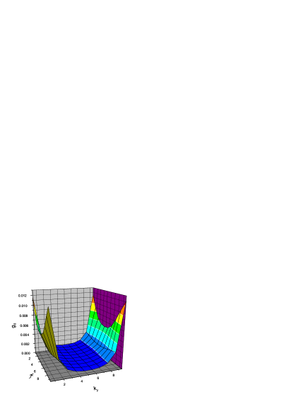
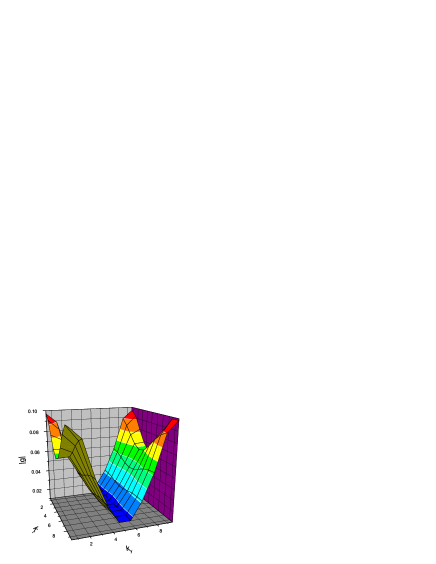
Figure 1: The values of $g_{0}$ (left figure) and $|g|$ (right figure) at $k_{1}=0$ in the semi - metal phase ($\beta=0.2$). The lattice size is $20^{3}$. Error bars are within $2\%$ of the considered quantities. We denote here $k_{t}=k_{4},k_{x}=k_{1},k_{y}=k_{2}$.

In the lattice regularized model with staggered fermions the single Grassman variable $\Psi$ is attached to the sites [31]. In terms of $\Psi$ the free fermion action has the form:

$$S=\sum_{x}\Bigl{(}m\,\bar{\Psi}_{x}\Psi_{x}+\frac{1}{2}\sum_{i=1,...,4}[\bar{\Psi}_{x}\alpha_{xi}\Psi_{x+\hat{i}}-\bar{\Psi}_{x+\hat{i}}\alpha_{xi}\Psi_{x}]\Bigr{)},\quad\alpha_{xi}=(-1)^{x_{1}+...+x_{i-1}}$$ (3)

In order to return to the original spinor and flavor indices of the spinors the lattice is considered with even number of lattice spacings in each direction [31]. Let us subdivide this lattice into the blocks consisted of elementary cubes. Each block has $2^{3}$ sites (two lattice sites in each direction). We denote the coordinates of the blocks by $y_{i}$. Therefore, the coordinates of the lattice sites are $x_{i}=2y_{i}+\eta_{i},\eta_{i}=0,1$. We define the new fields

$$[\Phi_{y}]^{\alpha}_{a}=\frac{1}{8}\sum_{\eta}[\Gamma_{1}^{\eta_{1}}\Gamma_{2}^{\eta_{2}}\Gamma_{4}^{\eta_{4}}]^{\alpha}_{a}\Psi_{2y+\eta}$$ (4)

Here index $\alpha=1,...,4$ is the spinor index while $a=1,...,4$ is the flavor index. Matrices $\Phi$ have $4\times 4$ components. But not all of these components are independent. Eq. (4) leads to the constraint

$$\Gamma_{3}\Gamma_{5}\Phi_{y}\Gamma_{5}\Gamma_{3}=\Phi_{y}$$ (5)

This constraint reduces the number of flavors from $4$ to $2$. The free propagator of $\Phi$ in momentum representation (of the blocked lattice) has the form (see [31] and also [30, 21]):

$$\tilde{\bf G}=\Bigl{(}\sum_{a}\Gamma_{a}\frac{1}{2}{\rm sin}\,k_{a}-i(m-\sum_{a}\frac{1}{2}(1-{\rm cos}\,k_{a})\Gamma_{5}\otimes T_{5}T_{a})\Bigr{)}^{-1}$$ (6)

$$= \frac{\frac{1}{2}\sum_{a}\Gamma_{a}{\rm sin}\,k_{a}+i(m-\frac{1}{2}\sum_{a}(1-{\rm cos}\,k_{a})\Gamma_{5}\otimes T_{5}T_{a})}{32[\sum_{a}\frac{1}{2}(1-{\rm cos}\,k_{a})+m^{2}]}$$

Here $T_{i}=\Gamma_{i}^{T}$ acts on the flavor indices while $\Gamma$ matrices act on the Dirac indices. Momenta $k$ are $k_{1}=\frac{2\pi K_{1}}{N/2}\,\quad k_{2}=\frac{2\pi K_{2}}{N/2}\,\quad k_{4}=\frac{2\pi K_{4}+\pi}{N/2},\quad K_{1},K_{2},K_{4}\in Z$; the lattice size is $N^{3}$. At the end of the calculation one must set $m=0$. The terms proportional to $(1-{\rm cos}\,k_{a})\sim k_{a}^{2}\sim a^{2}$ disappear in the continuum limit (the other terms are proportional to $\sim a$; here $a$ is the lattice spacing).

We suppose that when the interaction is switched on the form of the Green function is the same:

$$\tilde{\bf G}=g_{1}\Gamma_{1}+g_{2}\Gamma_{2}+g_{3}\Gamma_{4}+ig_{0}+ig^{a}_{5}\Gamma_{5}\otimes T_{5}T_{a}.$$ (7)

The terms proportional to $g^{a}_{5}$ are expected to be negligible in the continuum limit similar to the corresponding terms without the Coulomb interactions. The values of $g_{a},a=1,2,3$ can be calculated as

$$g_{a}(k) = \frac{i}{16N_{1}^{2}N_{2}^{2}N_{t}^{2}}\sum_{y,z}e^{ik(z-y)}\sum_{\eta,\eta^{\prime}}(-1)^{\eta_{1}+...+\eta_{a-1}}$$ (8)

$$\delta(\eta^{\prime}_{i}-[\eta_{i}+\delta_{ia}]{\rm mod}\,2)\langle G(2y+\eta,2z+\eta^{\prime})\rangle$$

Here $\langle G(2y+\eta,2z+\eta^{\prime})\rangle$ is the staggered fermion propagator in the external field averaged over the configurations of the $U(1)$ gauge field and over the pseudofermion configurations.

In addition we calculated the $g_{0}$ component of the Green function as follows:

$$g_{0}(k) = \frac{i}{16N_{1}^{2}N_{2}^{2}N_{t}^{2}}\sum_{y,z}e^{ik(z-y)}\sum_{\eta,\eta^{\prime}}\delta(\eta^{\prime}_{i}-[\eta_{i}+\delta_{ia}]{\rm mod}\,2)\langle G(2y+\eta,2z+\eta^{\prime})\rangle$$ (9)

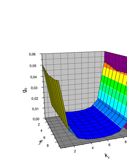
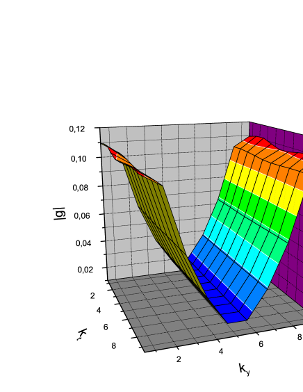
Figure 2: The values of $g_{0}$ (left figure) and $|g|$ (right figure) at $k_{1}=0$ close to the phase transition ($\beta=0.08$). The lattice size is $20^{3}$. Error bars are within $2\%$ of the considered quantities. We denote $k_{t}=k_{4},k_{x}=k_{1},k_{y}=k_{2}$.

3 Numerical results

We simulate the model at $m=0.01$. We collected enough statistics to calculate the Green functions over all momentum space at $\beta=0.05,0.07,0.08,0.09,0.1,0.2$ on the lattices $10^{3}$ and $20^{3}$. On the smaller lattice the Green functions are calculated using the direct inversion of matrices. On the larger lattice of size $20^{3}$ we calculated the Green function using the stochastic estimators (for the description of the method see [21]). According to [21, 16] the values $\beta=0.05,0.07,0.08$ belong to the insulator phase while the values $\beta=0.09,0.1,0.2$ belong to the semi - metal phase. We do not observe any qualitative dependence of the results on the lattice size.

We analyze the data on the values of the Green functions and have found that there is the essential excess of $|g|=\sqrt{g_{1}^{2}+g_{2}^{2}+g_{3}^{2}}$ at $k_{a}\sim 0\,(a=1,2,3)$ over the average value within the momentum space lattice for $\beta=0.2$. The dependence of this quantity on momentum is represented in Fig. 1. On this figure we represent the values of $|g|=\sqrt{g_{1}^{2}+g_{2}^{2}+g_{3}^{2}}$ and $g_{0}$ attached to the points of the dual lattice. The value at the point of the dual lattice is obtained via the averaging over the vertices of the corresponding cube of the original lattice. Namely, we plot the values $|g|=\sqrt{\frac{1}{24}\sum_{a,v}g_{a}(v)^{2}}$ and $g_{0}=\frac{1}{8}\sum_{v}g_{0}(v)$, where the sum is over the vertices $v$ of the given cube and over the components $a=1,2,3$. On this figure the four peaks represent the single one due to the periodic boundary conditions.

We observe that deep in the insulator phase (at $\beta=0.05$) the Green function practically does not depend on $k_{4}$. Moreover, $g_{3}$ is negligible compared to $g_{1}$ and $g_{2}$. This means that different time spices correlate with each other very weakly, and that the system is described by the effective $2D$ model rather than by the $2+1$ dimensional model. The dependence of the Green function on $k_{1},k_{2}$ demonstrates an essential excess of $|g|=\sqrt{g_{1}^{2}+g_{2}^{2}}$ at $k_{1}=k_{2}=0$ over the rest of the momentum space lattice. The value of $g_{0}$ at $k_{1}=k_{2}=0$ in the insulator phase is essentially larger than the value of $g_{0}$ in the semi - metal phase for $k_{4}=k_{1}=k_{2}=0$ (see Fig. 3; again, the values are attached to the points of the dual lattice and are averaged over the vertices of the corresponding cubes).

Close to the phase transition ($\beta=0.07,0.08,0.09,0.1$) the maxima of $|g|$ and $g_{0}$ as the functions of $k_{4}$ at $k_{4}=0,k_{1}=0,k_{2}=0$ are observed, in principle. However, the hights of these maxima are very small, while $|g|$ and $g_{0}$ depend on $k_{4}$ very weakly (see Fig. 2). That’s why at $m=0.01$ we observe smooth transition between the two regimes in the vicinity of the phase transition (its position is pointed out, for example, in [21, 16]). The first regime corresponds to the effective $2D$ description of the theory approached deep in the insulator phase. The second regime corresponds to the traditional semi - metal phase.

4 Conclusions

We have simulated the lattice regularized effective field model of graphene monolayer with the Coulomb interactions taken into account. We calculate the fermion Green function in momentum space. We consider several points on the phase diagram: deep in the the semi - metal phase, close to the position of the phase transition pointed out in [16, 21, 19, 23, 17, 18, 20], and deep in the insulator phase.

At $\beta=0.05$ (deep in the insulator phase) the Green function practically does not depend on $k_{4}$. This means that different time slices correlate very weakly. Moreover, the values of $g_{3}(k)\sim\langle\bar{\psi}(k)\Gamma_{4}\psi(k)\rangle$ are negligible compared with $g_{1},g_{2}$ for any values of the momentum $k$ (where $g_{1}(k)\sim\langle\bar{\psi}(k)\Gamma_{1}\psi(k)\rangle,\,\quad g_{2}\sim\langle\bar{\psi}(k)\Gamma_{2}\psi(k)\rangle$). This means that deep in the insulator phase the energy of the fermionic excitation tends to infinity. Close to the position of the phase transition semi - metal – insulator we observe the intermediate behavior of the mentioned above quantities. Namely, there are very small hights of the peaks of $|g|=\sqrt{g_{1}^{2}+g_{2}^{2}+g_{3}^{2}}$ and $g_{0}\sim\langle\bar{\psi}(k)\psi(k)\rangle$ as functions of $k_{4}$.

This is confirmed also by the consideration of the results for the current - current correlator as a function of imaginary time represented in [21] (Eq. (16)). Namely, in Fig. 3 of [21] the spectral density of this correlator is represented. It is clear from this Figure that in the insulator phase at $\epsilon<4$ (i.e., for $\beta<0.8$) the only maximum of the spectral density is at the frequencies $k_{4}\sim 1/a$, where $a$ is the lattice spacing. For $k_{4}<<1/a$ the values of the spectral density are much less than at $k_{4}\sim 1/a$. Therefore, the correlation time extracted from this correlator is of the order of the lattice spacing (in the insulator phase) .

We consider the mentioned above results as an indication that at the sufficiently small values of the dielectric permittivity of the substrate the effective low energy field model does not correspond to the original tight - binding model. Therefore, it may have nothing to do with the reality. Most likely, here the discreteness of the graphene honeycomb lattice becomes important for the description of the physical phenomena and the excitations that are not described by the effective field theory play an important role. Therefore the conclusion of [13, 14, 16, 21, 22, 19, 23, 17, 18, 20, 21] , that there is the insulator phase of the graphene monolayer, seems to us questionable.

It is worth mentioning that we measure our quantities at fixed $m=0.01$ while the phase transition was observed in the behavior of the quantities extrapolated to $m=0$. In order to make definite conclusions it is necessary to repeat the calculations described in the present paper for different values of $m$ and to extrapolate the results to the value of $m$ equal to zero. Also the dependence of the quantities on the lattice size has to be investigated. This should be a content of the further investigation.

To conclude let us mention the recent work [33], where the experimantal results are presented with no sign of the insulator phase in graphene.

The authors kindly acknowledge comments of M.I.Katsnelson, and a private communication with G.E.Volovik, as well as the discussions with the members of the lattice ITEP group M.I.Polikarpov, P.V.Buividovich, V.I.Zakharov, O.V.Pavlovsky. The numerical simulations have been performed using the facilities of the supercomputer centers of Moscow University, Kurchatov Institute, and ITEP. This work was partly supported by RFBR grant 11-02-01227 and by the Russian Ministry of Science and Education (program ”Human Capital” and the contract No. 07.514.12.4028).

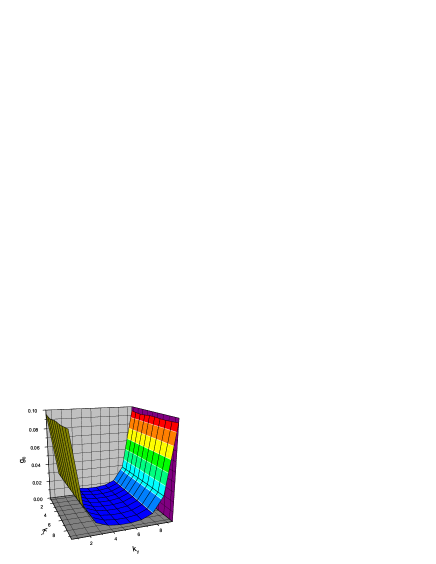
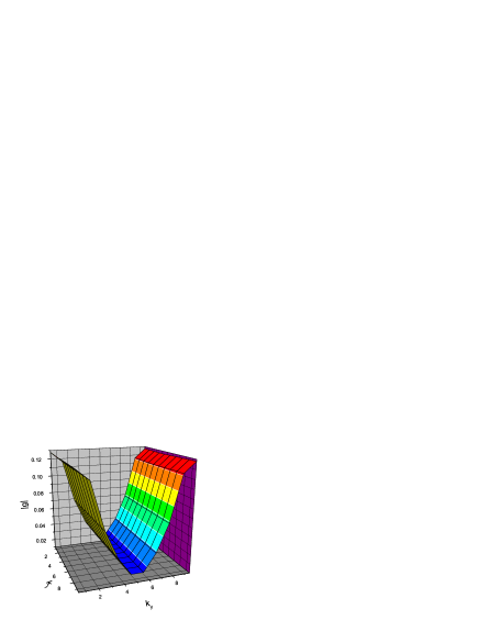
Figure 3: The values of $g_{0}$ (left figure) and $|g|$ (right figure) at $k_{1}=0$ in the insulator phase ($\beta=0.05$). The lattice size is $20^{3}$. Error bars are within $2\%$ of the considered quantities. We denote here $k_{t}=k_{4},k_{x}=k_{1},k_{y}=k_{2}$.

References

- [1] M.I. Katsnelson, Graphene: Carbon in Two Dimensions, Cambridge Univ. Press, Cambridge, 2012.
- [2] A. Shytov, M. Rudner, N. Gu, M. Katsnelson, L. Levitov, Solid State Commun. 149 (2009) 1087.
- [3] K.S. Novoselov, E. McCann, S.V. Morozov, V.I. Falko, M.I. Katsnelson, U. Zeitler, D. Jiang, F. Schedin, A.K. Geim, Nature Phys. 2 (2006) 177.
- [4] K. S. Novoselov, A. K. Geim, S. V. Morozov, D.Jiang, Y.Zhang, S. V.Dubonos, I. V.Grigorieva, and A. A. Firsov, Science 306, 666 (2004),
- [5] A. K. Geim K. S. Novoselov, Nature Materials, volume 6, 183 (2007), ArXiv:cond-mat/0702595.
- [6] I. V. Fialkovsky, D. V. Vassilevich , Quantum Field Theory in Graphene, talk at QFEXT 11, arXiv:1111.3017
- [7] P. R. Wallace, Phys. Rev. 71, 622 (1947).
- [8] A. H. Castro Neto, F. Guinea, N. M. R. Peres, K. S. Novoselov and A. K. Geim, The electronic properties of graphene, Rev. Mod. Phys. 81 , 109-162 (2009).
- [9] V. N. Kotov, B. Uchoa, and A. H. Castro Neto, Phys. Rev. B 78, 035119 (2008)
- [10] ”Interaction corrections to the polarization function of graphene ”, Inti Sodemann, Michael M. Fogler, arXiv:1206.3519
- [11] Gordon W. Semenoff, Chiral Symmetry Breaking in Graphene, Proceedings of the Nobel Symposium on Graphene and Quantum Matter, arXiv:1108.2945
- [12] D.T. Son, Quantum critical point in graphene approached in the limit of infinitely strong Coulomb interaction, Phys.Rev. B75 (2007) 235423, arXiv:cond-mat/0701501
- [13] Yasufumi Araki, Chiral Symmetry Breaking in Monolayer Graphene by Strong Coupling Expansion of Compact and Non-compact U(1) Lattice Gauge Theories, Annals Phys.326:1408-1424,2011, arXiv:1010.0847
- [14] Y. Araki , T. Hatsuda, Phys. Rev. B 82, 121403 (2010)
- [15] Y. Araki, Phys. Rev. B 85, 125436 (2012)
- [16] Joaquin E. Drut, Timo A. Lahde, Lattice field theory simulations of graphene, Phys. Rev. B 79, 165425 (2009), arXiv:0901.0584
- [17] J. E. Drut, T. A. Lähde, Phys. Rev. Lett. 102, 026802 (2009).
- [18] J. E. Drut, T. A. Lähde ,Phys. Rev. B 79, 241405 (2009).
- [19] J. E. Drut, T. A. Lähde,E. Tölö, PoS Lattice2010, 006 (2010).
- [20] J. E. Drut, T. A. Lähde,PoS Lattice2011, 074 (2011)
- [21] P. V. Buividovich, E. V. Luschevskaya, O. V. Pavlovsky, M. I. Polikarpov, M. V. Ulybyshev, ”Numerical study of the conductivity of graphene monolayer within the effective field theory approach”, arXiv:1204.0921, to appear in Phys.Rev.B
- [22] Wes Armour, Simon Hands, Costas Strouthos, Monte Carlo Simulation of the Semimetal-Insulator Phase Transition in Monolayer Graphene, Phys.Rev.B81:125105,2010, arXiv:0910.5646
- [23] W. Armour, S. Hands, and C. Strouthos, Phys. Rev. B 84,075123 (2011).
- [24] R. Brower, C. Rebbi and D. Schaich, Hybrid Monte Carlo simulation on the graphene hexagonal lattice, PoS LATTICE 2011, 056 (2011), arXiv:1204.5424
- [25] ”Magnetic Field Driven Metal-Insulator Phase Transition In Planar Systems”, E. V. Gorbar, V. P. Gusynin, V. A. Miransky, I. A. Shovkovy, Phys. Rev. B 66, 045108 (2002). ”Supercritical Coulomb center and excitonic instability in graphene”, O.V. Gamayun, E.V. Gorbar, V.P. Gusynin, Phys. Rev. B 80, 165429 (2009). ”Gap generation and semimetal-insulator phase transition in graphene”, O.V. Gamayun, E.V. Gorbar, V.P. Gusynin, Phys. Rev. B 81, 075429 (2010).
- [26] G.E. Volovik, The Universe in a Helium Droplet, Clarendon Press, Oxford (2003).
- [27] G.E. Volovik, in Quantum Analogues: From Phase Transitions to Black Holes and Cosmology, Eds. W.G. Unruh and R. Schutzhold, Springer Lecture Notes in Physics 718/2007, pp. 31-73; cond-mat/0601372.
- [28] G.E. Volovik, Topological invariants for Standard Model: from semi-metal to topological insulator, Pis’ma ZhETF 91, 61–67 (2010); JETP Lett. 91, 55–61 (2010); arXiv:0912.0502.
- [29] Yasuhiro Hatsugai, Topological aspect of graphene physics, Proceedings for HMF-19, arXiv:1008.4653
- [30] M.A.Zubkov, Fermi point in graphene as a monopole in momentum space, Pis’ma ZhETF 95, 168–174 (2012), arXiv:1112.2474
- [31] I.Montvay, G.Munster, Quantum fields on a lattice, Cambridge University press, 1994
- [32] M.I. Polikarpov, U.J. Wiese, and M.A. Zubkov, Phys. Lett. B 309, 133 (1993).
- [33] ”How close can one approach the Dirac point in graphene experimentally?” Alexander S. Mayorov, Daniel C. Elias, Ivan S. Mukhin, Sergey V. Morozov, Leonid A. Ponomarenko, Kostya S. Novoselov, A. K. Geim, Roman V. Gorbachev, arXiv:1206.3848