Global Optimal Solution to Discrete Value Selection Problem with Inequality Constraints

Abstract

This paper presents a canonical dual method for solving a quadratic discrete value selection problem subjected to inequality constraints. The problem is first transformed into a problem with quadratic objective and 0-1 integer variables. The dual problem of the 0-1 programming problem is thus constructed by using the canonical duality theory. Under appropriate conditions, this dual problem is a maximization problem of a concave function over a convex continuous space. Numerical simulation studies, including some large scale problems, are carried out so as to demonstrate the effectiveness and efficiency of the method proposed.

1 Introduction

Many decision making problems, such as portfolio selection, capital budgeting, production planning, resource allocation, and computer networks, can often be formulated as integer programming problems. See for examples, (Chen et al 2010; Floudas 2000; Karlof 2006). In engineering applications, the variables of these optimization problems can not have arbitrary values. Instead, some or all of the variables must be selected from a list of integer or discrete values for practical reasons. For examples, structural members may have to be selected from selections available in standard sizes, member thicknesses may have to be selected from the commercially available ones, the number of bolts for a connection must be an integer, the number of reinforcing bars in a concrete member must be an integer,etc (Huang and Arora 1997). However, these integer programming problems are computationally highly demanding. Nevertheless, some numerical methods are now available.

Several review articles on nonlinear optimization problems with discrete variables have been recently published (Arora et al. 1994; Loh and Papalambros 1991; Samdgren 1990; Thanedar and Vanderplaats 1994), and some popular methods have been discussed, including branch and bound methods, a hybrid method that combines a branch-and-bound method with a dynamic programming technique (Marsten and Morin 1978), sequential linear programming, rounding-off techniques, cutting plane techniques (Balas et al. 1993), heuristic techniques, penalty function approach and sequential linear programming. The relaxation method has also been proposed, leading to second order cone programming (SOC) (Ghaddar et al. 2011). More recently, simulated annealing (Kincaid and Padula 1990) and genetic algorithms have been discussed.

Branch and bound is perhaps the most widely known and used method for discrete optimization problems. When applied to linear problems, this method can be implemented in a way to yield a global minimum point; however, for nonlinear problems there is no such guarantee, unless the problem is convex. The branch and bound method has been used successfully to deal with problems with discrete design variables, however, for the problem with a large number of discrete design variables, the number of subproblems (nodes) becomes large, making the method inefficient.

Simulated annealing (SA) is a stochastic technique to find a global minimizer. The basic idea of the method is to generate a random point and evaluate the problem functions. If the trial point is feasible and the cost function value is smaller than the current best record, the point is accepted, and record for the best value is updated. The acceptance is based on value of the probability density function. In computing the probability a parameter called the temperature is used. Initially, a larger target value is selected. As the trials progress, the target value is reduced (this is called the cooling schedule), and the process is terminated after a fairly large number of trials. The main deficiency of the method is the unknown rate at which the target level is to be reduced and uncertainty in the total number of trials.

Genetic algorithms (GA) belong to the category of stochastic search methods (Holland 1975). In a GA, several design alternatives, called a population in a generation, are allowed to reproduce and cross among themselves, with bias allocated to the most fit members of the population. Three operators are needed to implement the algorithm: reproduction, crossover, and mutation. These three steps are repeated for successive generations of the population until certain stopping criteria are satisfied. The member in the final generation with the best fitness level is the optimum design.

The SA method and GA usually need large execution times to find a global minimum. Although it is possible to find the best solution if temperature is reduced slowly and enough execution time is allowed. A drawback of SA is lack of an effective stopping criterion. It is difficult to tell whether a global or fairly good solution has been reached. It is also important to note that the CPU times for SA and GA can vary from one run to the next for the same problem (Huang and Arora 1997).

Canonical duality theory provides a new and potentially useful methodology for solving a large class of integer programming problems. It was shown in (Gao 2007 and Fang et al 2008) that the Boolean integer programming problems are actually equivalent to certain canonical dual problems in continuous space without duality gap, which can be solved deterministically under certain conditions. This theory has been generalized for solving multi-integer programming and the well-known max cut problems (see Wang et al 2008 and Wang et al 2012). It is also shown in (Gao 2009, Gao and Ruan 2010) that by the canonical duality theory, the NP-hard quadratic integer programming problem can be transformed to a continuous unconstrained Lipschitzian global optimization problem, which can be solved via deterministic methods (see Gao et al 2012).

In this paper, our goal is to solve a general quadratic programming problem with its decision variables taking values from discrete sets. The elements from these discrete sets are not required to be binary or uniformly distributed. An effective numerical method is developed based on the canonical duality theory (Gao 2000). The rest of the paper is organized as follows. Section 2 presents a mathematical statement of the problem. Section 3 shows that this general discrete-value quadratic programming problem can be transformed into a 0-1 programming problem in higher dimensional space. In Section 4, the canonical duality is utilized to construct the canonical dual problem. The computational method, which is based on solving the canonical dual problem, is developed. Some numerical examples are illustrated to demonstrate the effectiveness and efficiency of the proposed method.The paper is ended with some concluding remarks.

2 Discrete Programming Problem

The discrete programming problem to be addressed is given below:

$$({\cal{P}}_{a})\;\; {\rm Minimize}\;\;P({\bf x})=\frac{1}{2}{\bf x}^{T}Q{\bf x}-{\bf c}^{T}{\bf x}$$

$${\rm subject\;to}\;\;{\bf g}({\bf x})={\bf A}{\bf x}-{\bf b}\leq 0,$$

$$\;\;\;\;\;\;\;\;\;\;\;\;\;\;\;\;\;{\bf x}=[x_{1},x_{2},\cdots,x_{n}]^{T},\;x_{i}\in U_{i},\;i=1,\cdots,n,$$

where $Q=\{q_{ij}\}\in{\mathbb{R}}^{n\times n}$ is an $n\times n$ positive semi-definite symmetric matrix, ${\bf A}=\{a_{ij}\}\in{\mathbb{R}}^{m\times n}$ is an $m\times n$ matrix with $rank({\bf A})=m<n$, ${\bf c}=[c_{1},\cdots,c_{n}]^{T}\in{\mathbb{R}}^{n}$ and ${\bf b}=[b_{1},\cdots,b_{m}]^{T}\in{\mathbb{R}}^{m}$ are given vectors. Here, for each $i=1,\cdots,n$,

$$U_{i}=\{u_{i,1},\cdots,u_{i,k_{i}}\},$$

where, $u_{i,j},j=1,\cdots,K_{i}$, are given real numbers. Let $K=\sum_{i=1}^{n}K_{i}$.

3 Equivalent Transformation

Let us introduce the following transformation,

$$x_{i}=\sum_{j=1}^{K_{i}}u_{i,j}y_{i,j},\;i=1,\cdots,n,$$ (3)

where, for each $i=1,\cdots,n$, $u_{i,j}\in U_{i},\;j=1,\cdots,K_{i}$. Then, the discrete programming problem $({\cal{P}}_{a})$ can be written as the following 0-1 programming problem:

$$({\cal{P}}_{b})\;\; {\rm Minimize}\;\;P({\bf y})=\frac{1}{2}{\bf y}^{T}B{\bf y}-{\bf h}^{T}{\bf y}$$ (7)

$${\rm subject\;to}\;\;{\bf g}({\bf y})=D{\bf y}-{\bf b}\leq 0,$$

$$\;\;\;\;\;\;\;\;\;\;\;\;\;\;\;\;\;\sum_{j=1}^{K_{i}}y_{ij}-1=0,\;i=1,\cdots,n,$$

$$\;\;\;\;\;\;\;\;\;\;\;\;\;\;\;\;\;y_{i,j}\in\{0,1\},~{}i=1,\ldots,n;\;j=1,\cdots,K_{i},$$

where

$${\bf y}=[y_{1,1},\cdots,y_{1,K_{1}},\cdots,y_{n,1},\cdots,y_{n,K_{n}}]^{T}\in{\mathbb{R}}^{K},$$

$${\bf h}=[c_{1}u_{1,1},\cdots,c_{1}u_{1,K_{1}},\cdots,c_{n}u_{n,1},\cdots,c_{n}u_{n,K_{n}}]^{T}\in{\mathbb{R}}^{K},$$

$$B=\left[\begin{array}[]{ccccc}q_{1,1}u_{1,1}^{2}&\cdots&q_{1,1}u_{1,1}u_{1,K_{1}}&\cdots&q_{1,n}u_{1,1}u_{n,K_{n}}\\ \vdots&\ddots&\vdots&\ddots&\vdots\\ q_{1,1}u_{1,K_{1}}u_{1,1}&\cdots&q_{1,1}u_{1,K_{1}}^{2}&\cdots&\cdots\\ \vdots&\ddots&\vdots&\ddots&\vdots\\ q_{n,1}u_{n,K_{n}}u_{1,1}&\cdots&\cdots&\cdots&q_{n,n}u_{n,K_{n}}^{2}\end{array}\right]\;\in{\mathbb{R}}^{K\times K},$$

$$D=\left[\begin{array}[]{ccccc}a_{1,1}u_{1,1}&\cdots&a_{1,1}u_{1,K_{1}}&\cdots&a_{1,n}u_{n,K_{n}}\\ \vdots&\ddots&\vdots&\ddots&\vdots\\ a_{m,1}u_{1,1}&\cdots&a_{m,1}u_{1,K_{1}}&\cdots&a_{m,n}u_{n,K_{n}}\end{array}\right]\;\in{\mathbb{R}}^{m\times K}.$$

Theorem 3.1

Problem $({\cal{P}}_{b})$ is equivalent to Problem $({\cal{P}}_{a})$.

Proof. For any $i=1,2,\cdots,n$, it is clear that constraints (7) and (7) are equivalent to the existence of only one $j\in\{1,\cdots,K_{i}\}$, such that $y_{i,j}=1$ while $y_{i,j}=0$ for all other $j$. Thus, from the definition of ${\bf y}$, the conclusion follows readily. $\Box$
Let

$$H=\left[\begin{array}[]{cccccccccc}1&\cdots&1&0&\cdots&0&\cdots&0&\cdots&0\\ 0&\cdots&0&1&\cdots&1&\cdots&0&\cdots&0\\ \vdots&\ddots&\vdots&\vdots&\ddots&\vdots&\ddots&\vdots&\ddots&\vdots\\ 0&\cdots&0&0&\cdots&0&\cdots&1&\cdots&1\end{array}\right]\in{\mathbb{R}}^{n\times K}$$

and, for any integer $N$, let

$${\bf e}_{N}=[1,\cdots,1,\cdots,1,\cdots,1]^{T}\in{\mathbb{R}}^{N}.$$

We consider the following quadratic programming problem:

$$({\cal{P}})\;\; {\rm Minimize}\;\;P({\bf y})=\frac{1}{2}{\bf y}^{T}B{\bf y}-{\bf h}^{T}{\bf y}$$ (14)

$${\rm subject\;to}\;\;{\bf g}({\bf y})=D{\bf y}-{\bf b}\leq 0,$$

$$\;\;\;\;\;\;\;\;\;\;\;\;\;\;\;\;\;H{\bf y}-{\bf e}_{n}=0,$$

$$\;\;\;\;\;\;\;\;\;\;\;\;\;\;\;\;\;{\bf y}\circ({\bf y}-{\bf e}_{K})\leq 0,$$

where the notation ${\bf s}\circ{\bf t}:=[s_{1}t_{1},s_{2}t_{2},\ldots,s_{K}t_{K}]^{T}$ denotes the Hadamard product for any two vectors ${\bf s},{\bf t}\in{\mathbb{R}}^{K}$.

4 Canonical duality theory: A brief review

The basic idea of the canonical duality theory can be demonstrated by solving the following general nonconvex problem (the primal problem $({\cal{P}})$ in short)

$$({\cal{P}}):\;\min_{x\in{\cal{X}}_{a}}\left\{P(x)=\frac{1}{2}\langle{\bf x},{\bf A}x\rangle-\langle x,{\bf f}\rangle+W(x)\right\},$$ (15)

where ${\bf A}\in{\mathbb{R}}^{n\times n}$ is a given symmetric indefinite matrix, ${\bf f}\in{\mathbb{R}}^{n}$ is a given vector, $\langle x,x^{*}\rangle$ denotes the bilinear form between $x$ and its dual variable $x^{*}$, ${\cal{X}}_{a}\subset{\mathbb{R}}^{n}$ is a given feasible space, and $W:{\cal{X}}_{a}\rightarrow{\mathbb{R}}\cup\infty$ is a general nonconvex objective function. The mathematical definition of the objectivity for general functions is given in (Gao, 2000).

The key step in the canonical dual transformation is to choose a nonlinear operator,

$$\mbox{\boldmath$\varepsilon$}={\Lambda}({\bf x}):{\cal{X}}_{a}\rightarrow{\cal{E}}_{a}\subset{\mathbb{R}}^{p}$$ (16)

and a canonical function $V:{\cal{E}}_{a}\rightarrow{\mathbb{R}}$ such that the nonconvex objective function $W({\bf x})$ can be recast by adopting a canonical form $W({\bf x})=V({\Lambda}({\bf x}))$. Thus, the primal problem $({\cal{P}})$ can be written in the following canonical form:

$$({\cal{P}}):\;\min_{{\bf x}\in{\cal{X}}_{a}}\left\{P({\bf x})=V({\Lambda}({\bf x}))-U({\bf x})\right\},$$ (17)

where $U({\bf x})=\langle{\bf x},{\bf f}\rangle-\frac{1}{2}\langle{\bf x},{\bf A}{\bf x}\rangle$. By the definition introduced in (Gao 2000), a differentiable function $V(\mbox{\boldmath$\varepsilon$})$ is said to be a canonical function on its domain ${\cal{E}}_{a}$ if the duality mapping $\mbox{\boldmath$\varsigma$}=\nabla V(\mbox{\boldmath$\varepsilon$})$ from ${\cal{E}}_{a}$ to its range ${\cal{S}}_{a}\subset{\mathbb{R}}^{p}$ is invertible. Let $\langle\mbox{\boldmath$\varepsilon$};\mbox{\boldmath$\varsigma$}\rangle$ denote the bilinear form on ${\mathbb{R}}^{p}$. Thus, for the given canonical function $V(\mbox{\boldmath$\varepsilon$})$, its Legendre conjugate $V^{*}(\mbox{\boldmath$\varsigma$})$ can be defined uniquely by the Legendre transformation

$$V^{*}(\mbox{\boldmath$\varsigma$})={\rm sta}\{\langle\mbox{\boldmath$\varepsilon$};\mbox{\boldmath$\varsigma$}\rangle-V(\mbox{\boldmath$\varepsilon$})\;|\;\;\mbox{\boldmath$\varepsilon$}\in{\cal{E}}_{a}\},$$ (18)

where the notation ${\rm sta}\{g(\mbox{\boldmath$\varepsilon$})|\;\mbox{\boldmath$\varepsilon$}\in{\cal{E}}_{a}\}$ stands for finding stationary point of $g(\mbox{\boldmath$\varepsilon$})$ on ${\cal{E}}_{a}$. It is easy to prove that the following canonical duality relations hold on ${\cal{E}}_{a}\times{\cal{S}}_{a}$:

$$\mbox{\boldmath$\varsigma$}=\nabla V(\mbox{\boldmath$\varepsilon$})\;\Leftrightarrow\;\mbox{\boldmath$\varepsilon$}=\nabla V^{*}(\mbox{\boldmath$\varsigma$})\;\Leftrightarrow V(\mbox{\boldmath$\varepsilon$})+V^{*}(\mbox{\boldmath$\varsigma$})=\langle\mbox{\boldmath$\varepsilon$};\mbox{\boldmath$\varsigma$}\rangle.$$ (19)

By this one-to-one canonical duality, the nonconvex term $W({\bf x})=V({\Lambda}({\bf x}))$ in the problem $({\cal{P}})$ can be replaced by $\langle{\Lambda}({\bf x});\mbox{\boldmath$\varsigma$}\rangle-V^{*}(\mbox{\boldmath$\varsigma$})$ such that the nonconvex function $P({\bf x})$ is reformulated as the so-called Gao and Strang total complementary function (Gao 2000):

$$\Xi({\bf x},\mbox{\boldmath$\varsigma$})=\langle{\Lambda}({\bf x});\mbox{\boldmath$\varsigma$}\rangle-V^{*}(\mbox{\boldmath$\varsigma$})-U({\bf x}).$$ (20)

By using this total complementary function, the canonical dual function $P^{d}(\mbox{\boldmath$\varsigma$})$ can be obtained as

$$P^{d}(\mbox{\boldmath$\varsigma$}) = {\rm sta}\{\Xi({\bf x},\mbox{\boldmath$\varsigma$})\;|\;{\bf x}\in{\cal{X}}_{a}\}$$ (21)

$$= U^{\Lambda}(\mbox{\boldmath$\varsigma$})-V^{*}(\mbox{\boldmath$\varsigma$}),$$

where $U^{\Lambda}({\bf x})$ is defined by

$$U^{\Lambda}(\mbox{\boldmath$\varsigma$})={\rm sta}\{\langle{\Lambda}({\bf x});\mbox{\boldmath$\varsigma$}\rangle-U({\bf x})\;|\;\;{\bf x}\in{\cal{X}}_{a}\}.$$ (22)

In many applications, the geometrically nonlinear operator ${\Lambda}({\bf x})$ is usually quadratic function

$${\Lambda}({\bf x})=\frac{1}{2}\langle{\bf x},D_{k}{\bf x}\rangle+\langle{\bf x},{\bf b}_{k}\rangle,$$ (23)

where $D_{k}\in{\mathbb{R}}^{n\times n}$ and ${\bf b}_{k}\in{\mathbb{R}}^{n}(k=1,\cdots,p)$. Let $\mbox{\boldmath$\varsigma$}=[\varsigma_{1},\cdots,\varsigma_{p}]^{T}$. In this case, the canonical dual function can be written in the following form:

$$P^{d}(\mbox{\boldmath$\varsigma$})=-\frac{1}{2}\langle{\bf F}(\mbox{\boldmath$\varsigma$}),{\bf G}(\mbox{\boldmath$\varsigma$}){\bf F}(\mbox{\boldmath$\varsigma$})\rangle-V^{\ast}(\mbox{\boldmath$\varsigma$}),$$ (24)

where ${\bf G}(\mbox{\boldmath$\varsigma$})={\bf A}+\sum_{k=1}^{p}\mbox{\boldmath$\varsigma$}_{k}D_{k}$, and ${\bf F}(\mbox{\boldmath$\varsigma$})={\bf f}-\sum_{k=1}^{p}\varsigma_{k}{\bf b}_{k}$.

Let ${\cal{S}}^{+}_{a}=\{\mbox{\boldmath$\varsigma$}\in{\mathbb{R}}^{p}|\;G(\mbox{\boldmath$\varsigma$})\succeq 0\}$. Therefore, the canonical dual problem can be proposed as

$$({\cal{P}}^{d}):\;\;\max\{P^{d}(\mbox{\boldmath$\varsigma$})|\;\;\mbox{\boldmath$\varsigma$}\in{\cal{S}}^{+}_{a}\}\vspace{-.3cm}.$$ (25)

which is a concave maximization problem over a convex set ${\cal{S}}^{+}_{a}\subset{\mathbb{R}}^{p}$.

Theorem 4.1 (Gao 2000)

Problem $({\cal{P}}^{d})$ is canonically dual to $({\cal{P}})$ in the sense that if $\bar{\mbox{\boldmath$\varsigma$}}$ is a critical point of $\Pi^{d}(\mbox{\boldmath$\varsigma$})$, then

$${\bar{\bf x}}={\bf G}^{\dagger}(\bar{\mbox{\boldmath$\varsigma$}})\mbox{\boldmath$\tau$}(\bar{\mbox{\boldmath$\varsigma$}})$$ (26)

is a critical point of $\Pi({\bf x})$ and

$$P({\bar{\bf x}})=\Xi({\bar{\bf x}},\bar{\mbox{\boldmath$\varsigma$}})=P^{d}(\bar{\mbox{\boldmath$\varsigma$}}).$$ (27)

If $\bar{\mbox{\boldmath$\varsigma$}}$ is a solution to $({\cal{P}}^{d})$, then ${\bar{\bf x}}$ is a global minimizer of $({\cal{P}})$ and

$$\min_{{\bf x}\in{{\cal{X}}_{a}}}P({\bf x})=\Xi({\bar{\bf x}},\bar{\mbox{\boldmath$\varsigma$}})=\max_{\mbox{\boldmath$\varsigma$}\in{\cal{S}}_{c}^{+}}P^{d}(\mbox{\boldmath$\varsigma$}).$$ (28)

Conversely, if ${\bar{\bf x}}$ is a solution to $({\cal{P}})$, it must be in the form of (26) for critical solution $\bar{\mbox{\boldmath$\varsigma$}}$ of $\Pi^{d}(\mbox{\boldmath$\varsigma$})$.

To help explain the theory, we consider a simple nonconvex optimization in ${\mathbb{R}}^{n}$:

$$\min\Pi({\bf x})=\frac{1}{2}\alpha(\frac{1}{2}\|{\bf x}\|^{2}-{\lambda})^{2}-{\bf x}^{T}{\bf f},\;\forall{\bf x}\in{\mathbb{R}}^{n},$$ (29)

where ${\alpha},{\lambda}>0$ are given parameters. The criticality condition $\nabla P({\bf x})=0$ leads to a nonlinear algebraic equation system in ${\mathbb{R}}^{n}$

$$\alpha(\frac{1}{2}\|{\bf x}\|^{2}-{\lambda}){\bf x}={\bf f}.$$ (30)

Clearly, to solve this n-dimensional nonlinear algebraic equation directly is difficult. Also traditional convex optimization theory can’t be used to identify global minimizer. However, by the canonical dual transformation, this problem can be solved. To do so, we let ${\mbox{\boldmath$\xi$}}={\Lambda}(u)=\frac{1}{2}\|{\bf x}\|^{2}-{\lambda}\in{\mathbb{R}}$. Then, the nonconvex function $W({\bf x})=\frac{1}{2}\alpha(\frac{1}{2}\|{\bf x}\|^{2}-{\lambda})^{2}$ can be written in canonical form $V({\mbox{\boldmath$\xi$}})=\frac{1}{2}\alpha{\mbox{\boldmath$\xi$}}^{2}$. Its Legendre conjugate is given by $V^{\ast}(\varsigma)=\frac{1}{2}\alpha^{-1}\varsigma^{2}$, which is strictly convex. Thus, the total complementary function for this nonconvex optimization problem is

$$\Xi({\bf x},\varsigma)=(\frac{1}{2}\|{\bf x}\|^{2}-{\lambda})\varsigma-\frac{1}{2}\alpha^{-1}\varsigma^{2}-{\bf x}^{T}{\bf f}.$$ (31)

For a fixed $\varsigma\in{\mathbb{R}}$, the criticality condition $\nabla_{{\bf x}}\Xi({\bf x})=0$ leads to

$$\varsigma{\bf x}-{\bf f}=0.$$ (32)

For each $\varsigma\neq 0$, the equation (32) gives ${\bf x}={\bf f}/\varsigma$ in vector form. Substituting this into the total complementary function $\Xi$, the canonical dual function can be easily obtained as

$$\Pi^{d}(\varsigma) = \{\Xi({\bf x},\varsigma)|\nabla_{{\bf x}}\Xi({\bf x},\varsigma)=0\}$$ (33)

$$= -\frac{{\bf f}^{T}{\bf f}}{2\varsigma}-\frac{1}{2}\alpha^{-1}\varsigma^{2}-{\lambda}\varsigma,\;\;\;\forall\varsigma\neq 0.$$

The critical point of this canonical function is obtained by solving the following dual algebraic equation

$$(\alpha^{-1}\varsigma+{\lambda})\varsigma^{2}=\frac{1}{2}{\bf f}^{T}{\bf f}.$$ (34)

For any given parameters $\alpha$, ${\lambda}$ and the vector ${\bf f}\in{\mathbb{R}}^{n}$, this cubic algebraic equation has at most three roots satisfying $\varsigma_{1}\geq 0\geq\varsigma_{2}\geq\varsigma_{3}$, and each of these roots leads to a critical point of the nonconvex function $P({\bf x})$, i.e., ${\bf x}_{i}={\bf f}/\varsigma_{i}$, $i=1,2,3$. By the fact that $\varsigma_{1}\in{\cal{S}}^{+}_{a}=\{\varsigma\in{\mathbb{R}}\;|\;\varsigma>0\}$, then Theorem 1 tells us that ${\bf x}_{1}$ is a global minimizer of $\Pi({\bf x})$. Consider one dimension problem with $\alpha=1$, ${\lambda}=2$, $f=\frac{1}{2}$, the primal function and canonical dual function are shown in Fig. 1, where, $x_{1}=2.11491$ is global minimizer of $P({\bf x})$, $\varsigma_{1}=0.236417$ is global maximizer of $\Pi^{d}(\mbox{\boldmath$\varsigma$})$, and $\Pi(x_{1})=-1.02951=\Pi^{d}(\varsigma_{1})$ (See the two black dots).

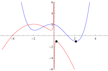
Figure 1: Graphs of the primal function $\Pi({\bf x})$ (blue) and its canonical dual function $\Pi^{d}(\varsigma)$ (red).

The canonical duality theory was original developed from general nonconvex systems. The canonical dual transformation can be used to convert a nonconvex problem into a canonical dual problem without duality gap, while the classical dual approaches may suffer from having a potential gap (Rockafellar 1987). The complementary-dual principle provides a unified form of analytical solutions to general nonconvex problems in either continuous or discrete systems. The canonical duality theory has shown its potential for various classes of challenging problems. A comprehensive review of the canonical duality theory and its applications can be found in (Gao and Ruan 2008; Gao and Ruan 2010; Gao et al. 2012; Gao et al. 2009; Gao et al. 2010; Ruan et al. 2010).

5 Canonical Dual Problem

Now we apply the canonical duality theory to integer programming problem presented in Section 2.

Let

$$U({\bf y})=-P({\bf y})={\bf h}^{T}{\bf y}-\frac{1}{2}{\bf y}^{T}B{\bf y},$$

and define

$${\bf z} = \Lambda({\bf y})=[(D{\bf y}-{\bf b})^{T},(H{\bf y}-{\bf e}_{n})^{T},({\bf y}\circ({\bf y}-{\bf e}_{K}))^{T}]^{T}$$

$$= [({\mbox{\boldmath$\epsilon$}})^{T},(\mbox{\boldmath$\delta$})^{T},(\mbox{\boldmath$\rho$})^{T}]^{T}\in{\mathbb{R}}^{m+n+K},$$

where $\Lambda$ is the so-called geometric operator. Let

$$W({\bf z})=\left\{\begin{array}[]{ll}0&\mbox{ if }{\mbox{\boldmath$\epsilon$}}\leq 0,\mbox{\boldmath$\delta$}=0,\mbox{\boldmath$\rho$}\leq 0,\\ +\infty&\mbox{ otherwise}.\end{array}\right.$$

Let ${\bf z}^{*}=[(\mbox{\boldmath$\sigma$})^{T},(\mbox{\boldmath$\tau$})^{T},(\mbox{\boldmath$\mu$})^{T}]^{T}\in{\mathbb{R}}^{m+n+K}$ be the canonical dual variables corresponding to those from the set $Z=\{({\mbox{\boldmath$\epsilon$}},\mbox{\boldmath$\delta$},\mbox{\boldmath$\rho$}):{\mbox{\boldmath$\epsilon$}}\leq 0,\mbox{\boldmath$\delta$}=0,\mbox{\boldmath$\rho$}\leq 0\}.$ Then, the Fenchel super-conjugate of the function $W({\bf z})$ is defined by

$$W^{\sharp}({\bf z}^{*}) = \sup\{{\bf z}^{T}{\bf z}^{*}-W({\bf z}):\;{\bf z}\in Z\}$$ (38)

$$= \left\{\begin{array}[]{ll}0&\mbox{ if }\mbox{\boldmath$\sigma$}\geq 0,\mbox{\boldmath$\mu$}\geq 0,\\ +\infty&\mbox{ otherwise}.\end{array}\right.$$

Let

$$G(\mbox{\boldmath$\mu$})=B+2{\mbox{Diag }}(\mbox{\boldmath$\mu$}),$$ (39)

and

$$F(\mbox{\boldmath$\sigma$},\mbox{\boldmath$\tau$},\mbox{\boldmath$\mu$})={\bf h}-D^{T}\mbox{\boldmath$\sigma$}-H^{T}\mbox{\boldmath$\tau$}+\mbox{\boldmath$\mu$}.$$ (40)

Then, the total complementary function can be obtained as:

$$\Xi({\bf y},\mbox{\boldmath$\sigma$},\mbox{\boldmath$\tau$},\mbox{\boldmath$\mu$}) = \langle\Lambda({\bf y}),{\bf z}^{*}\rangle-W^{\sharp}({\bf z}^{*})-U({\bf y})$$

$$= \frac{1}{2}{\bf y}^{T}B{\bf y}-{\bf h}^{T}{\bf y}+\mbox{\boldmath$\sigma$}^{T}(D{\bf y}-{\bf b})$$

$$+\mbox{\boldmath$\tau$}^{T}(H{\bf y}-{\bf e}_{n})+\mbox{\boldmath$\mu$}^{T}({\bf y}\circ({\bf y}-{\bf e}_{K}))$$

$$= \frac{1}{2}{\bf y}^{T}B{\bf y}+\frac{1}{2}{\bf y}^{T}(2{\mbox{Diag }}(\mbox{\boldmath$\mu$})){\bf y}-{\bf h}^{T}{\bf y}$$

$$(D^{T}\mbox{\boldmath$\sigma$})^{T}{\bf y}-\mbox{\boldmath$\mu$}^{T}{\bf y}+(H^{T}\mbox{\boldmath$\tau$})^{T}{\bf y}-\mbox{\boldmath$\sigma$}^{T}{\bf b}-\mbox{\boldmath$\tau$}^{T}{\bf e}_{n}$$

$$= \frac{1}{2}{\bf y}^{T}G(\mbox{\boldmath$\mu$}){\bf y}-F^{T}(\mbox{\boldmath$\sigma$},\mbox{\boldmath$\tau$},\mbox{\boldmath$\mu$}){\bf y}-\mbox{\boldmath$\sigma$}^{T}{\bf b}-\mbox{\boldmath$\tau$}^{T}{\bf e}_{n}.$$

The critical condition $\nabla_{{\bf y}}\Xi({\bf y},\mbox{\boldmath$\sigma$},\mbox{\boldmath$\tau$},\mbox{\boldmath$\mu$})=0$ leads to

$${\bf y}=G^{\dagger}(\mbox{\boldmath$\mu$})F(\mbox{\boldmath$\sigma$},\mbox{\boldmath$\tau$},\mbox{\boldmath$\mu$}),$$ (41)

where $G^{\dagger}(\mbox{\boldmath$\mu$})$ denotes the Moore-Penrose generalized inverse of $G(\mbox{\boldmath$\mu$})=(B+2{\mbox{Diag }}(\mbox{\boldmath$\mu$}))$.

The canonical dual problem can be stated as follows:

$$({\cal{P}}^{d})\;\; {\rm Maximize}\;\;P^{d}(\mbox{\boldmath$\sigma$},\mbox{\boldmath$\tau$},\mbox{\boldmath$\mu$})=-\frac{1}{2}F(\mbox{\boldmath$\sigma$},\mbox{\boldmath$\tau$},\mbox{\boldmath$\mu$})^{T}G^{\dagger}(\mbox{\boldmath$\mu$})F(\mbox{\boldmath$\sigma$},\mbox{\boldmath$\tau$},\mbox{\boldmath$\mu$})-\mbox{\boldmath$\sigma$}^{T}{\bf b}-\mbox{\boldmath$\tau$}^{T}{\bf e}_{n}$$

$${\rm subject\;to}\;\;\mbox{\boldmath$\sigma$}\geq 0,\mbox{\boldmath$\mu$}>0,$$

$$\;\;\;\;\;\;\;\;\;\;\;\;\;\;\;\;\;\mbox{\boldmath$\sigma$}\in{\mathbb{R}}^{m},\mbox{\boldmath$\tau$}\in{\mathbb{R}}^{n},\mbox{\boldmath$\mu$}\in{\mathbb{R}}^{K}.$$

Theorem 5.1 (Complementary-Dual Principle)

Problem $({\cal{P}}^{d})$ is a canonically dual to Problem $({\cal{P}})$ in the sense that if $(\bar{\mbox{\boldmath$\sigma$}},\bar{\mbox{\boldmath$\tau$}},\bar{\mbox{\boldmath$\mu$}})$ is a KKT solution of Problem $({\cal{P}}^{d})$, then the vector

$$\bar{\bf y}(\bar{\mbox{\boldmath$\sigma$}},\bar{\mbox{\boldmath$\tau$}},\bar{\mbox{\boldmath$\mu$}})=G^{\dagger}(\bar{\mbox{\boldmath$\mu$}})F(\bar{\mbox{\boldmath$\sigma$}},\bar{\mbox{\boldmath$\tau$}},\bar{\mbox{\boldmath$\mu$}})$$ (42)

is a KKT solution of Problem $({\cal{P}})$ and

$$P(\bar{\bf y})=P^{d}(\bar{\mbox{\boldmath$\sigma$}},\bar{\mbox{\boldmath$\tau$}},\bar{\mbox{\boldmath$\mu$}}).$$

Moreover, if $(\bar{\mbox{\boldmath$\sigma$}},\bar{\mbox{\boldmath$\tau$}},\bar{\mbox{\boldmath$\mu$}})$ is a critical point of Problem $({\cal{P}}^{d})$ and $\bar{\mbox{\boldmath$\mu$}}>0$, then $\bar{\bf y}$ is a critical point of Problem $({\cal{P}})$.

Proof. By introducing the Lagrange multiplier vector ${\mbox{\boldmath$\epsilon$}}\leq 0\in{\mathbb{R}}^{m}$, $\mbox{\boldmath$\delta$}\in{\mathbb{R}}^{n}$, and $\mbox{\boldmath$\rho$}\leq 0\in{\mathbb{R}}^{K}$, the Lagrangian function associated with the dual function $P^{d}(\mbox{\boldmath$\sigma$},\mbox{\boldmath$\tau$},\mbox{\boldmath$\mu$})$ becomes

$$L(\mbox{\boldmath$\sigma$},\mbox{\boldmath$\tau$},\mbox{\boldmath$\mu$},{\mbox{\boldmath$\epsilon$}},\mbox{\boldmath$\delta$},\mbox{\boldmath$\rho$})=P^{d}(\mbox{\boldmath$\sigma$},\mbox{\boldmath$\tau$},\mbox{\boldmath$\mu$})-{\mbox{\boldmath$\epsilon$}}^{T}\mbox{\boldmath$\sigma$}+\mbox{\boldmath$\delta$}^{T}\mbox{\boldmath$\tau$}-\mbox{\boldmath$\rho$}^{T}\mbox{\boldmath$\mu$}.$$

Then, the KKT conditions of the dual problem become

$$\frac{\partial L(\mbox{\boldmath$\sigma$},\mbox{\boldmath$\tau$},\mbox{\boldmath$\mu$},{\mbox{\boldmath$\epsilon$}},\mbox{\boldmath$\delta$},\mbox{\boldmath$\rho$})}{\partial\mbox{\boldmath$\sigma$}} = D{\bf y}-{\bf b}-{\mbox{\boldmath$\epsilon$}}=0,$$

$$\frac{\partial L(\mbox{\boldmath$\sigma$},\mbox{\boldmath$\tau$},\mbox{\boldmath$\mu$},{\mbox{\boldmath$\epsilon$}},\mbox{\boldmath$\delta$},\mbox{\boldmath$\rho$})}{\partial\mbox{\boldmath$\tau$}} = H{\bf y}-{\bf e}_{n}+\mbox{\boldmath$\delta$}=0,$$

$$\frac{\partial L(\mbox{\boldmath$\sigma$},\mbox{\boldmath$\tau$},\mbox{\boldmath$\mu$},{\mbox{\boldmath$\epsilon$}},\mbox{\boldmath$\delta$},\mbox{\boldmath$\rho$})}{\partial\mbox{\boldmath$\mu$}} = {\bf y}\circ({\bf y}-{\bf e}_{K})-\mbox{\boldmath$\rho$}=0,$$

$$\mbox{\boldmath$\sigma$}\geq 0,{\mbox{\boldmath$\epsilon$}}\leq 0,\mbox{\boldmath$\sigma$}^{T}{\mbox{\boldmath$\epsilon$}} = 0,$$

$$\mbox{\boldmath$\mu$}\geq 0,\mbox{\boldmath$\rho$}\leq 0,\mbox{\boldmath$\mu$}^{T}\mbox{\boldmath$\rho$} = 0.$$

They can be written as:

$$D{\bf y}\leq{\bf b},$$ (43)

$$H{\bf y}-{\bf e}_{n}=0,$$ (44)

$${\bf y}({\bf y}-{\bf e}_{K})\leq 0,$$ (45)

$$\mbox{\boldmath$\sigma$}\geq 0,\mbox{\boldmath$\sigma$}^{T}(D{\bf y}-{\bf b})=0,$$ (46)

$$\mbox{\boldmath$\mu$}\geq 0,\mbox{\boldmath$\mu$}^{T}({\bf y}\circ({\bf y}-{\bf e}_{K}))=0.$$ (47)

Specifically, if $\mbox{\boldmath$\mu$}>0$, the complementary condition leads to ${\bf y}\circ({\bf y}-{\bf e}_{K})=0$. This proves that if $(\bar{\mbox{\boldmath$\sigma$}},\bar{\mbox{\boldmath$\tau$}},\bar{\mbox{\boldmath$\mu$}})$ is a KKT solution of $({\cal{P}}^{d})$, then (43)-(45) is the so-called primal feasibility condition, while (46)-(47) is the so-called dual feasibility condition and complementary slackness condition. Therefore, the vector

$$\bar{\bf y}(\bar{\mbox{\boldmath$\sigma$}},\bar{\mbox{\boldmath$\tau$}},\bar{\mbox{\boldmath$\mu$}})=G^{\dagger}(\bar{\mbox{\boldmath$\mu$}})F(\bar{\mbox{\boldmath$\sigma$}},\bar{\mbox{\boldmath$\tau$}},\bar{\mbox{\boldmath$\mu$}})$$

is a KKT solution of Problem $({\cal{P}})$.

Again, by the complementary condition and (42), we have

$$P^{d}(\mbox{\boldmath$\sigma$},\mbox{\boldmath$\tau$},\mbox{\boldmath$\mu$}) = -\frac{1}{2}F(\mbox{\boldmath$\sigma$},\mbox{\boldmath$\tau$},\mbox{\boldmath$\mu$})^{T}G(\mbox{\boldmath$\tau$})^{\dagger}F(\mbox{\boldmath$\sigma$},\mbox{\boldmath$\tau$},\mbox{\boldmath$\mu$})-\mbox{\boldmath$\sigma$}^{T}{\bf b}-\mbox{\boldmath$\tau$}^{T}{\bf e}_{n}$$

$$= \frac{1}{2}{\bf y}^{T}B{\bf y}-{\bf h}^{T}{\bf y}+\mbox{\boldmath$\sigma$}^{T}(D{\bf y}-{\bf b})+\mbox{\boldmath$\tau$}(H{\bf y}-{\bf e}_{n})+\mbox{\boldmath$\mu$}({\bf y}\circ({\bf y}-{\bf e}_{K}))$$

$$= \frac{1}{2}{\bf y}^{T}B{\bf y}-{\bf h}^{T}{\bf y}=P({\bf y}).$$

$\Box$

To continue, let the feasible space ${\cal{Y}}$ of problem $({\cal{P}})$ and the dual feasible space ${\cal{Z}}$ be defined by

$${\cal{Y}}=\{{\bf y}\in{\mathbb{R}}^{K}:D{\bf y}\leq b,H{\bf y}={\bf e}_{n},{\bf y}\circ({\bf y}-{\bf e}_{K})\leq 0\}$$

and

$${\cal{Z}}=\{(\mbox{\boldmath$\sigma$},\mbox{\boldmath$\tau$},\mbox{\boldmath$\mu$})\in{\mathbb{R}}^{m}\times{\mathbb{R}}^{n}\times{\mathbb{R}}^{K}:\mbox{\boldmath$\sigma$}\geq 0,\mbox{\boldmath$\mu$}>0,F(\bar{\mbox{\boldmath$\sigma$}},\bar{\mbox{\boldmath$\tau$}},\bar{\mbox{\boldmath$\mu$}})\in{\cal{C}}_{ol}(G(\mbox{\boldmath$\mu$}))\},$$

respectively, where ${\cal{C}}_{ol}(G(\mbox{\boldmath$\mu$}))$ denotes the linear space spanned by the columns of $G(\mbox{\boldmath$\mu$})$.

We introduce a subset of the dual feasible space:

$${\cal{Z}}_{a}^{+}:=\{(\mbox{\boldmath$\sigma$},\mbox{\boldmath$\tau$},\mbox{\boldmath$\mu$})\in{\cal{Z}}:G(\mbox{\boldmath$\mu$})\succ 0\}.$$ (48)

We have the following theorem.

Theorem 5.2

Assume that $(\bar{\mbox{\boldmath$\sigma$}},\bar{\mbox{\boldmath$\tau$}},\bar{\mbox{\boldmath$\mu$}})$ is a critical point of $P^{d}(\mbox{\boldmath$\sigma$},\mbox{\boldmath$\tau$},\mbox{\boldmath$\mu$})$ and $\bar{\bf y}=G^{\dagger}(\bar{\mbox{\boldmath$\mu$}})F(\bar{\mbox{\boldmath$\sigma$}},\bar{\mbox{\boldmath$\tau$}},\bar{\mbox{\boldmath$\mu$}})$. If $(\bar{\mbox{\boldmath$\sigma$}},\bar{\mbox{\boldmath$\tau$}},\bar{\mbox{\boldmath$\mu$}})\in{\cal{Z}}_{a}^{+}$, then $\bar{\bf y}$ is a global minimizer of $P({\bf y})$ and $(\bar{\mbox{\boldmath$\sigma$}},\bar{\mbox{\boldmath$\tau$}},\bar{\mbox{\boldmath$\mu$}})$ is a global maximizer of $P^{d}(\mbox{\boldmath$\sigma$},\mbox{\boldmath$\tau$},\mbox{\boldmath$\mu$})$ with

$$P(\bar{\bf y})=\min_{{\bf y}\in{\cal{Y}}}P({\bf y})=\max_{(\mbox{\boldmath$\sigma$},\mbox{\boldmath$\tau$},\mbox{\boldmath$\mu$})\in{\cal{Z}}_{a}^{+}}P^{d}(\mbox{\boldmath$\sigma$},\mbox{\boldmath$\tau$},\mbox{\boldmath$\mu$})=P^{d}(\bar{\mbox{\boldmath$\sigma$}},\bar{\mbox{\boldmath$\tau$}},\bar{\mbox{\boldmath$\mu$}})$$ (49)

Proof

The canonical dual function $P^{d}(\mbox{\boldmath$\sigma$},\mbox{\boldmath$\tau$},\mbox{\boldmath$\mu$})$ is concave on ${\cal{Z}}_{a}^{+}$. Therefore, a critical point $(\bar{\mbox{\boldmath$\sigma$}},\bar{\mbox{\boldmath$\tau$}},\bar{\mbox{\boldmath$\mu$}})\in{\cal{Z}}_{a}^{+}$ must be a global maximizer of $P^{d}(\mbox{\boldmath$\sigma$},\mbox{\boldmath$\tau$},\mbox{\boldmath$\mu$})$ on ${\cal{Z}}_{a}^{+}$. For any given $(\mbox{\boldmath$\sigma$},\mbox{\boldmath$\tau$},\mbox{\boldmath$\mu$})\in{\cal{Z}}_{a}^{+}$, the complementary function $\Xi({\bf y},\mbox{\boldmath$\sigma$},\mbox{\boldmath$\tau$},\mbox{\boldmath$\mu$})$ is convex in ${\bf y}$ and concave in $(\mbox{\boldmath$\sigma$},\mbox{\boldmath$\tau$},\mbox{\boldmath$\mu$})$, the critical point $(\bar{\bf y},\bar{\mbox{\boldmath$\sigma$}},\bar{\mbox{\boldmath$\tau$}},\bar{\mbox{\boldmath$\mu$}})$ is a saddle point of the complementary function. More specifically, we have

$$P^{d}(\bar{\mbox{\boldmath$\sigma$}},\bar{\mbox{\boldmath$\tau$}},\bar{\mbox{\boldmath$\mu$}}) = \max_{(\mbox{\boldmath$\sigma$},\mbox{\boldmath$\tau$},\mbox{\boldmath$\mu$})\in{\cal{Z}}_{a}^{+}}P^{d}(\mbox{\boldmath$\sigma$},\mbox{\boldmath$\tau$},\mbox{\boldmath$\mu$})$$

$$= \max_{(\mbox{\boldmath$\sigma$},\mbox{\boldmath$\tau$},\mbox{\boldmath$\mu$})\in{\cal{Z}}_{a}^{+}}\min_{{\bf y}\in{\cal{Y}}}\Xi({\bf y},\mbox{\boldmath$\sigma$},\mbox{\boldmath$\tau$},\mbox{\boldmath$\mu$})=\min_{{\bf y}\in{\cal{Y}}}\max_{(\mbox{\boldmath$\sigma$},\mbox{\boldmath$\tau$},\mbox{\boldmath$\mu$})\in{\cal{Z}}_{a}^{+}}\Xi({\bf y},\mbox{\boldmath$\sigma$},\mbox{\boldmath$\tau$},\mbox{\boldmath$\mu$})$$

$$= \min_{{\bf y}\in{\cal{Y}}}\max_{(\mbox{\boldmath$\sigma$},\mbox{\boldmath$\tau$},\mbox{\boldmath$\mu$})\in{\cal{Z}}_{a}^{+}}\{\frac{1}{2}{\bf y}^{T}G(\mbox{\boldmath$\mu$}){\bf y}-({\bf h}-D^{T}\mbox{\boldmath$\sigma$}-H^{T}\mbox{\boldmath$\tau$}+\mbox{\boldmath$\mu$})^{T}{\bf y}$$

$$-\mbox{\boldmath$\sigma$}^{T}{\bf b}-\mbox{\boldmath$\tau$}^{T}{\bf e}_{n}\}$$

$$= \min_{{\bf y}\in{\cal{Y}}}\max_{(\mbox{\boldmath$\sigma$},\mbox{\boldmath$\tau$},\mbox{\boldmath$\mu$})\in{\cal{Z}}_{a}^{+}}\{\frac{1}{2}{\bf y}^{T}B{\bf y}-{\bf h}^{T}{\bf y}+\mbox{\boldmath$\sigma$}^{T}(D{\bf y}-{\bf b})$$

$$+\mbox{\boldmath$\tau$}^{T}(H{\bf y}-{\bf e}_{n})+\mbox{\boldmath$\mu$}^{T}{\bf y}\circ({\bf y}-{\bf e}_{K})\}$$

$$= \min_{{\bf y}\in{\cal{Y}}}\max_{(\mbox{\boldmath$\sigma$},\mbox{\boldmath$\tau$},\mbox{\boldmath$\mu$})\in{\cal{Z}}_{a}^{+}}\{\frac{1}{2}{\bf y}^{T}B{\bf y}-{\bf h}^{T}{\bf y}+({\bf z}^{*})^{T}{\bf z}\}$$

Note that

$$\max_{{\bf z}^{*}\in{\cal{Z}}_{a}^{+}}\{W^{\sharp}({\bf z}^{*})\}=0$$

and

$$\max_{{\bf z}\in Z}\{W({\bf z})\}=0.$$

Thus, it follows from (5) that

$$P^{d}(\bar{\mbox{\boldmath$\sigma$}},\bar{\mbox{\boldmath$\tau$}},\bar{\mbox{\boldmath$\mu$}}) = \min_{{\bf y}\in{\cal{Y}}}\max_{(\mbox{\boldmath$\sigma$},\mbox{\boldmath$\tau$},\mbox{\boldmath$\mu$})\in{\cal{Z}}_{a}^{+}}\{\frac{1}{2}{\bf y}^{T}B{\bf y}-{\bf h}^{T}{\bf y}+({\bf z}^{*})^{T}{\bf z}-W^{\sharp}({\bf z}^{*})\}$$

$$= \min_{{\bf y}\in{\cal{Y}}}\{\frac{1}{2}{\bf y}^{T}B{\bf y}-{\bf h}^{T}{\bf y}\}+\max_{(\mbox{\boldmath$\sigma$},\mbox{\boldmath$\tau$},{\bf u})\in{\cal{Z}}_{a}^{+}}\{({\bf z}^{*})^{T}{\bf z}-W^{\sharp}({\bf z}^{*})\}$$

$$= \min_{{\bf y}\in{\cal{Y}}}\{\frac{1}{2}{\bf y}^{T}B{\bf y}-{\bf h}^{T}{\bf y}\}+\max_{(\mbox{\boldmath$\sigma$},\mbox{\boldmath$\tau$},\mbox{\boldmath$\mu$})\in{\cal{Z}}_{a}^{+}}\{({\bf z}^{*})^{T}{\bf z}-{\bf z}^{T}{\bf z}^{*}+W({\bf z})\}$$

$$= \min_{{\bf y}\in{\cal{Y}}}\{\frac{1}{2}{\bf y}^{T}B{\bf y}-{\bf h}^{T}{\bf y}\}$$

$$= \min_{{\bf y}\in{\cal{Y}}}P({\bf y}).$$

This completes the proof. $\Box$

6 Numerical Experience

All data and computational results presented in this section are produced by Matlab. In order to save space and fit the matrix in the paper, we round our these results up to two decimals.

Example 1. 5-dimensional problem.

Consider Problem $({\cal{P}}_{a})$ with ${\bf x}=[x_{1},\cdots,x_{5}]^{T}$ , while $x_{i}\in\{2,3,5\}$, $i=1,\cdots,5$,

$${\bf Q}=\left[\begin{array}[]{ccccc}3.43&0.60&0.39&0.10&0.60\\ 0.60&2.76&0.32&0.65&0.49\\ 0.39&0.32&2.07&0.59&0.39\\ 0.10&0.65&0.59&2.62&0.30\\ 0.60&0.49&0.39&0.30&3.34\end{array}\right],$$

$${\bf c}=[38.97,-24.17,40.39,-9.65,13.20]^{T},$$

$${\bf A}=\left[\begin{array}[]{ccccc}0.94&0.23&0.04&0.65&0.74\\ 0.96&0.35&0.17&0.45&0.19\\ 0.58&0.82&0.65&0.55&0.69\\ 0.06&0.02&0.73&0.30&0.18\end{array}\right],$$

$${\bf b}=[11.49,9.32,14.43,5.66]^{T}.$$

Under the transformation (3), this problem is transformed into the 0-1 programming Problem $({\cal{P}})$, where

$${\bf y}=[y_{1,1},y_{1,2},y_{1,3},\cdots,y_{5,1},y_{5,1},y_{5,3}]^{T}\in{\mathbb{R}}^{15},$$

$${\bf B}=\left[\begin{array}[]{ccccccccccccccc}13.71&20.56&34.27&2.40&3.61&6.01&1.58&2.37&3.95&0.39&0.58&0.97&2.38&3.57&5.95\\ 20.56&30.84&51.41&3.61&5.41&9.01&2.37&3.55&5.92&0.58&0.88&1.46&3.57&5.36&8.93\\ 34.27&51.41&85.68&6.01&9.01&15.02&3.95&5.92&9.87&0.97&1.46&2.43&5,95&8.93&14.88\\ 2.40&3.61&6.01&11.05&16.57&27.61&1.27&1.91&3.18&2.61&3.91&6.52&1.95&2.93&4.88\\ 3.61&5.41&9.01&16.57&24.85&41.42&1.91&2.86&4.77&3.91&5.87&9.78&2.93&4.39&7.32\\ 6.01&9.01&15.02&27.61&41.42&69.03&3.18&4.77&7.96&6.52&9.78&16.31&4.88&7.32&12.20\\ 1.58&2.37&3.95&1.27&1.91&3.18&8.27&12.40&20.67&2.37&3.55&5.92&1.57&2.36&3.93\\ 2.37&3.55&5.92&1.91&2.86&4.77&12.40&18.60&31.00&3.55&5.33&8.89&2.36&3.53&5.90\\ 3.95&5.92&9.87&3.18&4.77&7.96&20.67&31.00&51.67&5.92&8.86&14.81&3.93&5.90&9.83\\ 0.39&5.58&0.97&2.61&3.91&6.52&2.37&3.55&5.92&10.50&15.74&26.24&1.20&1.80&3.00\\ 0.58&0.88&1.46&3.91&5.87&9.78&3.55&5.33&8.89&15.74&23.62&39.36&1.80&2.70&4.50\\ 0.97&1.46&2.43&6.52&9.78&16.31&5.92&8.89&14.81&26.24&39.36&65.60&3.00&4.50&7.51\\ 2.38&3.57&5.95&1.95&2.93&4.88&1.57&2.36&3.93&1.20&1.80&3.00&13.35&20.02&33.37\\ 3.57&5.36&8.93&2.93&4.39&7.32&2.36&3.54&5.90&1.80&2.70&4.50&20.02&30.04&50.06\\ 5.95&8.93&14.88&4.88&7.32&12.20&3.93&5.90&9.83&3.00&4.50&7.51&33.37&50.06&83.43\end{array}\right],$$

$${\bf h} = [77.95,116.92,194.87,-48.34,-72.51,-120.85,80.78,121.17$$

$$201.96,-19.29,-28.94,-48.23,26.39,39.59,65.99]^{T},$$

$${\bf D}=\left[\begin{array}[]{ccccccccccccccc}\;1.88\;\;2.83\;\;4.71\;\;0.47\;\;0.70\;\;1.17\;\;0.09\;\;0.12\;\;0.22\;\;1.30\;\;1.94\;\;3.24\;\;1.49\;\;2.23\;\;3.72\\ \;1.91\;\;2.87\;\;4.78\;\;0.71\;\;1.06\;\;1.77\;\;0.34\;\;0.51\;\;0.85\;\;0.90\;\;1.35\;\;2.25\;\;0.38\;\;0.57\;\;0.94\\ \;1.15\;\;1.72\;\;2.88\;\;1.64\;\;2.46\;\;4.11\;\;1.30\;\;1.95\;\;3.25\;\;1.09\;\;1.64\;\;2.74\;\;1.37\;\;2.06\;\;3.43\\ \;0.12\;\;0.18\;\;0.30\;\;0.03\;\;0.05\;\;0.08\;\;1.46\;\;2.20\;\;3.66\;\;0.59\;\;0.89\;\;1.48\;\;0.37\;\;0.55\;\;0.92\end{array}\right],$$

$${\bf H}=\left[\begin{array}[]{cccccccccc}1&\cdots&1&0&\cdots&0&\cdots&0&\cdots&0\\ 0&\cdots&0&1&\cdots&1&\cdots&0&\cdots&0\\ \vdots&\ddots&\vdots&\vdots&\ddots&\vdots&\ddots&\vdots&\ddots&\vdots\\ 0&\cdots&0&0&\cdots&0&\cdots&1&\cdots&1\end{array}\right]\in{\mathbb{R}}^{5\times 15}.$$

The Canonical dual problem can be stated as follows:

$$({\cal{P}}^{d})\;\; {\rm Maximize}\;\;P^{d}(\mbox{\boldmath$\sigma$},\mbox{\boldmath$\tau$},\mbox{\boldmath$\mu$})=-\frac{1}{2}F(\mbox{\boldmath$\sigma$},\mbox{\boldmath$\tau$},\mbox{\boldmath$\mu$})^{T}G^{\dagger}(\mbox{\boldmath$\mu$})F(\mbox{\boldmath$\sigma$},\mbox{\boldmath$\tau$},\mbox{\boldmath$\mu$})-\mbox{\boldmath$\sigma$}^{T}{\bf b}-\mbox{\boldmath$\tau$}^{T}{\bf e}_{5}$$

$${\rm subject\;to}\;\;\mbox{\boldmath$\sigma$}\geq 0,\mbox{\boldmath$\mu$}>0,$$

$$\;\;\;\;\;\;\;\;\;\;\;\;\;\;\;\;\;\mbox{\boldmath$\sigma$}\in{\mathbb{R}}^{4},\mbox{\boldmath$\tau$}\in{\mathbb{R}}^{5},\mbox{\boldmath$\mu$}\in{\mathbb{R}}^{15},$$

where $F(\mbox{\boldmath$\sigma$},\mbox{\boldmath$\tau$},\mbox{\boldmath$\mu$})$ and $G(\mbox{\boldmath$\mu$})$ are as defined by (39) and (40), respectively.
By solving this dual problem with the sequential quadratic programming method in the optimization Toolbox within the Matlab environment, we obtain

$$\bar{\mbox{\boldmath$\sigma$}}=[0,0,0,0]^{T},$$

$$\bar{\mbox{\boldmath$\tau$}}=[73.90,-106.70,111.95,-59.27,-0.01]^{T},$$

and

$$\bar{\mbox{\boldmath$\mu$}} = [39.34,22.07,12.49,33.56,3.01,76.14,61.00,35.52$$

$$18.78,1.47,41.96,0.001,0.001,0.006]^{T}.$$

It is clear that $(\bar{\mbox{\boldmath$\sigma$}},\bar{\mbox{\boldmath$\tau$}},\bar{\mbox{\boldmath$\mu$}})\in{\cal{Z}}_{a}^{+}$. Thus, from Theorem 5.2,

$$\bar{\bf y} = (B+2{\mbox{Diag }}(\bar{\mbox{\boldmath$\mu$}}))^{\dagger}({\bf h}-D^{T}\bar{\mbox{\boldmath$\sigma$}}-H^{T}\bar{\mbox{\boldmath$\tau$}}+\bar{\mbox{\boldmath$\mu$}})$$

$$= [0,0,1,1,0,0,0,0,1,1,0,0,1,0,0]^{T}$$

is the global minimizer of Problem $({\cal{P}})$ with $P^{d}(\bar{\mbox{\boldmath$\sigma$}},\bar{\mbox{\boldmath$\tau$}},\bar{\mbox{\boldmath$\mu$}})=-227.87=P(\bar{\bf y})$. The solution to the original primal problem can be calculated by using the transformation

$$\bar{x}_{i}=\sum_{j=1}^{K_{i}}u_{i,j}\bar{y}_{i,j},\;i=1,2,3,4,5,$$

to give

$${\bar{\bf x}}=[5,2,5,2,2]^{T}$$

with $P({\bar{\bf x}})=-227.87$.

Example 2. 10-dimensional problem.

Consider Problem $({\cal{P}}_{a})$, with ${\bf x}=[x_{1},\cdots,x_{10}]^{T}$, while $x_{i}\in\{1,2,4,7,9\},\;i=1,\cdots,10$,

$${\bf Q}=\left[\begin{array}[]{cccccccccc}6.17&0.62&0.46&0.37&0.56&0.66&0.67&0.85&0.57&0.44\\ 0.62&5.63&0.29&0.56&0.79&0.29&0.43&0.69&0.49&0.39\\ 0.46&0.29&5.81&0.55&0.22&0.55&0.36&0.27&0.51&0.91\\ 0.37&0.56&0.55&6.10&0.28&0.42&0.44&0.34&0.75&0.44\\ 0.56&0.79&0.22&0.28&4.75&0.40&0.55&0.42&0.49&0.44\\ 0.66&0.29&0.55&0.42&0.40&5.71&0.32&0.57&0.65&0.70\\ 0.67&0.43&0.36&0.44&0.55&0.32&5.27&0.56&0.37&0.85\\ 0.85&0.69&0.27&0.34&0.42&0.57&0.56&5.91&0.15&0.62\\ 0.57&0.49&0.51&0.75&0.49&0.65&0.37&0.15&4.51&0.46\\ 0.44&0.39&0.91&0.44&0.44&0.70&0.85&0.62&0.46&5.73\end{array}\right],$$

$${\bf f}=[0.89,0.03,0.49,0.17,0.98,0.71,0.50,0.47,0.06,0.68]^{T},$$

$${\bf A}=\left[\begin{array}[]{cccccccccc}0.04&0.82&0.97&0.83&0.83&0.42&0.02&0.20&0.05&0.94\\ 0.07&0.72&0.65&0.08&0.80&0.66&0.98&0.49&0.74&0.42\\ 0.52&0.15&0.80&0.13&0.06&0.63&0.17&0.34&0.27&0.98\\ 0.10&0.66&0.45&0.17&0.40&0.29&0.11&0.95&0.42&0.30\\ 0.82&0.52&0.43&0.39&0.53&0.43&0.37&0.92&0.55&0.70\end{array}\right],$$

$${\bf b}=[33.76,37.07,26.75,25.46,37.36]^{T}.$$

By solving the canonical dual problem of Problem $({\cal{P}}_{a})$, we obtain

$$\bar{\mbox{\boldmath$\sigma$}}=[0,0,0,0,0]^{T},$$

$$\bar{\mbox{\boldmath$\tau$}} = [-19.99,-20.12,-18.13,-18.37,-14.32,$$

$$-17.13,-18.46,-19.73,-17.65,-16.55]^{T},$$

and

$$\bar{\mbox{\boldmath$\mu$}} = [9.51,0.97,21.93,53.36,74.34,9.95,0.21,20.53,51.01,71.35$$

$$8.68,0.77,19.68,48.03,66.94,8.30,1.77,21.91,52.13,72.27$$

$$6.40,1.54,17.39,41.19,57.04,7.57,1.98,21.10,49.77,68.90$$

$$9.15,0.16,18.79,46.72,65.34,9.82,0.09,19.90,49.63,69.45$$

$$8.76,0.13,17.92,44.60,62.39,6.26,4.03,24.60,55.48,76.04]^{T},$$

It is clear that $(\bar{\mbox{\boldmath$\sigma$}},\bar{\mbox{\boldmath$\tau$}},\bar{\mbox{\boldmath$\mu$}})\in{\cal{Z}}_{a}^{+}$. Therefore,

$$\bar{\bf y}=[1,0,0,0,0,1,0,0,0,0,1,0,0,0,0,1,0,0,0,0,1,0,0,0,0,$$

$$1,0,0,0,0,1,0,0,0,0,1,0,0,0,0,1,0,0,0,0,1,0,0,0,0]^{T}$$

is the global minimizer of the problem $({\cal{P}})$ with $P^{d}(\bar{\mbox{\boldmath$\sigma$}},\bar{\mbox{\boldmath$\tau$}},\bar{\mbox{\boldmath$\mu$}})=45.54=P(\bar{\bf y})$. The solution to the original primal problem is

$${\bar{\bf x}}=[1,1,1,1,1,1,1,1,1,1]^{T}$$

with $P({\bar{\bf x}})=45.54$.

Example 3. Large scale problems.

Consider Problem $({\cal{P}}_{a})$ with $n=20$, $50$, $100$, $200$ and $300$. Let these five problems be referred to as Problem (1), $\cdots$, Problem (5), respectively. Their coefficients are generated randomly with uniform distribution. For each problem, $q_{ij}\in(0,1)$, $a_{ij}\in(0,1)$, for $i=1,\cdots,n$; $j=1,\cdots,n$, and $c_{i}\in(0,1)$, $x_{i}\in\{1,2,3,4,5\}$, for $i=1,\cdots n$. Without loss of generality, we ensure that the constructed $Q$ is a symmetric matrix. Otherwise, we let $Q=\frac{Q+Q^{T}}{2}$. Furthermore, let $Q$ be such that it is diagonally dominated. For each $x_{i}$, its lower bound is $l_{i}=1$, and its upper bound is $u_{i}=5$. Let $l=[l_{1},\cdots,l_{n}]^{T}$ and $u=[u_{1},\cdots,u_{n}]^{T}$. The right-hand sides of the linear constraints are chosen such that the feasibility of the test problem is satisfied. More specifically, we set ${\bf b}=\sum_{j}a_{ij}l_{j}+0.5\cdot(\sum_{j}a_{ij}u_{j}-\sum_{j}a_{ij}l_{j})$.

We then construct the canonical problem of each of the five problems. It is solved by using the sequential quadratic programming method with active set strategy from the Optimization Toolbox within the Matlab environment. The specifications of the personal notebook computer used are: Intel(R), Core(TM)(1.20 GHZ), Window Vista(TM). Table 1 presents the numerical results, where $m$ is number of linear constraints in Problem $I({\cal{P}}_{a})$.

Table 1: Numerical results for large scale integer programming problems

n	m	CPU Time (Seconds)
20	5	4.8
50	5	19.1
100	5	75.8
200	5	277.8
300	5	649.7

From Table 1, we see that the algorithm based on the canonical dual method can solve large scale problems with reasonable computational time. Furthermore, for each of the five problems, the solution obtained is a global optimal solution. For the case of $n=300$, the equivalent problem in the form of Problem $({\cal{P}}_{b})$ has 1500 variables. For such a problem, there are $2^{1500}$ possible combinations.

7 Conclusion

We have presented a canonical duality theory for solving a general discrete value selection problem with quadratic cost function and linear constraints. Our results show that this NP-hard problem can be converted to a continuous concave dual maximization problem without duality gap. If the canonical dual space ${\cal{Z}}^{+}_{a}$ is non empty, the problem can be solved easily via well-developed convex optimization methods. Several examples, including some large scale ones, were solved effectively by using the method proposed.

Acknowledgement: This paper was partially supported by a grant (AFOSR FA9550-10-1-0487) from the US Air Force Office of Scientific Research. Dr. Ning Ruan was supported by a funding from the Australian Government under the Collaborative Research Networks (CRN) program.

References

(1) Arora JS, Huang MW, Hsieh CC (1994)
Methods for optimization of nonlinear problems with discrete
variables: a review. Struct. Optim. 8: 69-85
(2) Balas E, Ceria S, Cornujols G (1993)
A lift-and-project cutting plane algorithm for mixed 0-1 programs.
Math. Program. 58: 295-324
(3) Chen, DS, Batson RG, Dang Y (2010)
Applied Integer Programming: Modeling and Solution. John Wiley and Sons
(4) Fang SC, Gao DY, Sheu RL, Wu SY(2008)
Canonical dual approach to solving 0-1 quadratic programming problems.
J. Ind. and Manag. Optim. 4(1):125-142
(5) Floudas CA(2000)
Nonlinear and Mixed-Integer Optimization: Theory, Methods and Applications.
Kluwer Academic, Dordrechi
(6) Gao DY (2000)
Duality Principles in Nonconvex Systems: Theory, Methods and
Applications, Kluwer Academic Publishers, Dordrecht/Boston/London
(7) Gao DY(2007)
Solutions and Optimality Criteria to Box Constrained
Nonconvex Minimization Problem. J. Ind. and Manag. Optim. 3(2): 293-304
(8) Gao DY, Ruan N (2008)
Solutions and optimality criteria for nonconvex quadratic-exponential
minimization problem. Math. Method. of Oper. Res. 67, pp 479-496
(9) Gao DY (2009)