Continuum particle-vibration coupling method in coordinate-space representation for finite nuclei

Abstract

In this paper we present a new formalism to implement the nuclear particle-vibration coupling (PVC) model. The key issue is the proper treatment of the continuum, that is allowed by the coordinate space representation. Our formalism, based on the use of zero-range interactions like the Skyrme forces, is microscopic and fully self-consistent. We apply it to the case of neutron single-particle states in ⁴⁰Ca, ²⁰⁸Pb and ²⁴O. The first two cases are meant to illustrate the comparison with the usual (i.e., discrete) PVC model. However, we stress that the present approach allows to calculate properly the effect of PVC on resonant states. We compare our results with those from experiments in which the particle transfer in the continuum region has been attempted. The latter case, namely ²⁴O, is chosen as an example of a weakly-bound system. Such a nucleus, being double-magic and not displaying collective low-lying vibrational excitations, is characterized by quite pure neutron single-particle states around the Fermi surface.

I Introduction

The accurate description of the single-particle (s.p.) strength in atomic nuclei is, to a large extent, an open issue (for a recent discussion see, e.g., Ref. open ). Whereas in light nuclei either ab-initio or shell model calculations are feasible, in the case of medium-heavy nuclei we miss a fully microscopic theory that is able to account for the experimental findings. Modern self-consistent models (either based on the mean-field Hamiltonians or on some implementation of Density Functional Theory) do not reproduce, as a rule, the level density around the Fermi surface. The reader can see, as a recent example, the results shown in Ref. stoitsov . Moreover, the fragmentation of the s.p. strength is by definition outside the framework of those models.

In the past decades, much emphasis has been put on the impact on the s.p. properties provided by the coupling with various collective nuclear motions. The basic ideas leading to particle-vibration coupling (PVC) models in spherical nuclei, or particle-rotation coupling models in deformed systems, have been discussed in textbooks BMII . These couplings provide dynamical content to the standard shell model, in keeping with the fact that the average potential becomes nonlocal in time or, in other words, frequency- or energy-dependent. We will call self-energy, in what follows, the dynamical part of the mean potential arising from vibrational coupling. This contribution will be added to the static Hartree-Fock (HF) potential. In this way, one may be able to describe the fragmentation and the related spectroscopic factors of the s.p. states, their density (which is proportional to the effective mass $m^{*}$ near the Fermi energy), the s.p. spreading widths, and the imaginary component of the optical potential.

In, e.g., the review article CM one can find a detailed discussion about the points mentioned in the previous paragraph, together with the relevant equations and the results of many calculations performed in the 80’s for the single-particle strength (mainly in ²⁰⁸Pb). These calculations are mostly not self-consistent and it is hard to extract from them quantitative conclusions because of the various approximations involved. Certainly, they all agree qualitatively in pointing out that PVC plays a decisive role to bring the density of levels near the Fermi energy in better agreement with experiment or, in other words, the effective mass $m^{*}$ close to the empirical value $m^{*}\approx m$.

This enhancement of the effective mass around the Fermi energy, as compared to the HF value, is only one example of a phenomenon that can be explained by assuming that single-particle and vibrational degrees of freedom are not independent. Other examples, although not treated in the current work, are worth to be mentioned in this Introduction. Several works have identified the exchange of vibrational quanta (phonons) between particles as one important mechanism responsible for nuclear pairing gori ; kamerdjev . In the approach of pastore ; idini and references therein, one aims at explaining the properties of superfluid nuclei by taking into account both the pairing induced by the phonon exchange and the self-energy mentioned above (cf. also the discussion in Refs. duguet ; baldo . We also remark that important developments are under way aiming at implementing ab-initio calculation schemes for open shell nuclei, based on self-consistent Green’s functions soma or on the unitary correlation operator method ucom ). Along the same line, more complicated processes can be explained by starting from elementary single-particle and vibrational degrees of freedom, and treating their coupling within the framework of an appropriate field theory: the spreading width of nuclear giant resonances, or the anharmonicity of two-phonon states (to mention only a few examples). The development of such a general many-body perturbation theory scheme could not avoid, so far, to resort to various approximations. In particular most of the calculations have employed simple, phenomenological coupling Hamiltonians.

Recently, in order to calculate the s.p. strength, microscopic PVC calculations have become available, either based on the nonrelativistic Skyrme Hamiltonian colo10 or on Relativistic Mean Field (RMF) parameterizations litvinova ; anatolj . The results seem to be satisfactory, in a qualitative or semi-quantitative sense, as they point to an increase of the effective mass around the Fermi energy. The results are clearly sensitive to the collectivity of the low-lying phonons produced by the self-consistent calculations. It is still unclear whether the results will eventually be improved by a re-fitting of the effective interactions or by the inclusion of higher-order processes.

One of the limitations of all the PVC models that have been introduced so far, lies in the fact that they discretize the s.p. continuum (clearly, this means that the description of the vibrations themselves relies on the same approximation). Although in Ref. varenna a scheme to calculate the self-energy in coordinate-space representation had been proposed, there is at present no available result for the s.p. strength (let alone more complex physical observables) that avoids the continuum discretization. Consequently, the goal of the present work is to introduce for the first time a consistent description of PVC with a proper treatment of the continuum. In order to achieve this, the coordinate space representation is used. The current work is based on previous experience on how to treat the continuum within the linear response theory or Random Phase Approximation (RPA) (see Refs. matsuo1 ; mizuyama ; Bertsch1 ; Bertsch2 ; Liu ).

The outline of the paper is as follows. In Sec. II, we describe our formalism starting from the general formulation and stressing the implementation of proper continuum treatment. The main goal of the section is to display the equations that we have implemented and solved, and discuss the s.p. level density. In Sec. III, the results for our three nuclei of choice are presented and discussed; whenever possibile, they are compared with experimental data. Finally, we summarize the paper and draw our conclusions in Sec. IV. Some details of the calculations are shown in a few Appendices.

II Formalism

II.1 Dyson equation in coodinate space representation.

The particle-vibration coupling (PVC) Hamiltonian CM ; Fetter ; Richard in coordinate space can be written as

$$\hat{H}_{PVC}=\int\!\!\!d\mbox{\boldmath$r$}\ \delta\hat{\rho}(\mbox{\boldmath$r$})\kappa(\mbox{\boldmath$r$})\sum_{\sigma}\hat{\psi}^{\dagger}(\mbox{\boldmath$r$}\sigma)\hat{\psi}(\mbox{\boldmath$r$}\sigma).$$

The density variation operator $\delta\hat{\rho}(\mbox{\boldmath$r$})\equiv\hat{\rho}(\mbox{\boldmath$r$})-\langle\hat{\rho}(\mbox{\boldmath$r$})\rangle$ (where the brackets denote the ground-state expectation value) in second quantized form is given by

$$\delta\hat{\rho}(\mbox{\boldmath$r$})=\sum_{n\lambda}\left[\delta\rho_{n\lambda}(\mbox{\boldmath$r$})\hat{\Gamma}^{\dagger}_{n\lambda}+\delta\rho^{*}_{n\lambda}(\mbox{\boldmath$r$})\hat{\Gamma}_{n\lambda}\right],$$ (2)

where $\hat{\Gamma}^{\dagger}_{n\lambda}$ and $\hat{\Gamma}_{n\lambda}$ are the creation and annihilation operators, respectively, of a phonon $n$ having multipolarity $\lambda$ and $\delta\rho_{n\lambda}$ is the corresponding transition density, whereas $\kappa$ is the residual force.

If the total Hamiltonian is $\hat{H}=\hat{H}_{0}+\hat{H}_{PVC}$, where the term $\hat{H}_{0}$ describes uncoupled s.p. states and vibrations, the many-body perturbation theory Fetter ; Richard can be applied. In particular, we assume that $\hat{H}_{0}$ includes the HF Hamiltonian for the nucleons and the independent boson Hamiltonian for the phonons (based on their RPA energies). We treat the term $\hat{H}_{PVC}$ as a perturbation using the interaction picture. We define Green’s functions in space-time representation and we apply standard tools like the Wick’s theorem to obtain the Dyson equation in terms of the unperturbed HF Green’s function $G_{0}$ and the perturbed Green’s functions $G$:

$$G(\mbox{\boldmath$r$}\sigma t,\mbox{\boldmath$r$}^{\prime}\sigma^{\prime}t^{\prime})=G_{0}(\mbox{\boldmath$r$}\sigma t,\mbox{\boldmath$r$}^{\prime}\sigma^{\prime}t^{\prime})+\sum_{\sigma_{1}\sigma_{2}}\int\!\!\!\int\!\!\!dt_{1}dt_{2}\int\!\!\!\int\!\!\!d\mbox{\boldmath$r$}_{1}d\mbox{\boldmath$r$}_{2}G_{0}(\mbox{\boldmath$r$}\sigma t,\mbox{\boldmath$r$}_{1}\sigma_{1}t_{1})\Sigma(\mbox{\boldmath$r$}_{1}\sigma_{1}t_{1},\mbox{\boldmath$r$}_{2}\sigma_{2}t_{2})G(\mbox{\boldmath$r$}_{2}\sigma_{2}t_{2},\mbox{\boldmath$r$}^{\prime}\sigma^{\prime}t^{\prime}).$$ (3)

The HF Green’s function satisfies $(\omega-\hat{h}_{0})G_{0}=1$, where $\hat{h}_{0}$ is the s.p. HF Hamiltonian. The self-energy function is defined by

$$\Sigma(\mbox{\boldmath$r$}_{1}\sigma_{1}t_{1},\mbox{\boldmath$r$}_{2}\sigma_{2}t_{2})=\kappa(\mbox{\boldmath$r$}_{1})G(\mbox{\boldmath$r$}_{1}\sigma_{1}t_{1},\mbox{\boldmath$r$}_{2}\sigma_{2}t_{2})\kappa(\mbox{\boldmath$r$}_{2})iR(\mbox{\boldmath$r$}_{1}t_{1},\mbox{\boldmath$r$}_{2}t_{2}),$$ (4)

where $R(\mbox{\boldmath$r$}_{1}t_{1}\mbox{\boldmath$r$}_{2}t_{2})$ is the RPA response function (or phonon propagator) in the space-time representation, and is defined by Fetter

$$iR(\mbox{\boldmath$r$}t,\mbox{\boldmath$r$}^{\prime}t^{\prime})=\langle\Psi_{RPA}|\mbox{T}\{\delta\hat{\rho}(\mbox{\boldmath$r$}t)\delta\hat{\rho}(\mbox{\boldmath$r$}^{\prime}t^{\prime})\}|\Psi_{RPA}\rangle,$$ (5)

where $T$ denotes the time-ordered product and the formula stresses that the phonons are defined using the RPA vacuum $|\Psi_{RPA}\rangle$ since this is exactly the phonon vacuum. We also note that the use of the Wick’s theorem in the derivation of Eq. (3) implies the use of the causal representation of the Green’s functions $G$ and $G_{0}$, as well as of the RPA response function $R$. The connection between the causal representation with the retarded and advanced representations is outlined in the Appendices, where the causal functions will be denoted by $G^{C},R^{C}$. This label will be omitted in the main text, where we shall only make use of the causal functions.

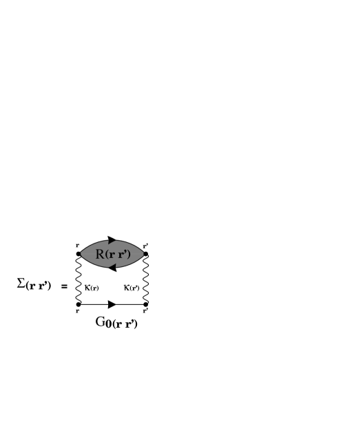
Figure 1: The Feynman diagram for the self-energy function which corresponds to Eq. (7), in the approximation in which $G_{0}$ replaces $G$.

The Fourier transform of Eq. (3) is given by

$$G(\mbox{\boldmath$r$}\sigma,\mbox{\boldmath$r$}^{\prime}\sigma^{\prime};\omega)=G_{0}(\mbox{\boldmath$r$}\sigma,\mbox{\boldmath$r$}^{\prime}\sigma^{\prime};\omega)+\sum_{\sigma_{1}\sigma_{2}}\int\!\!\!\int\!\!\!d\mbox{\boldmath$r$}_{1}d\mbox{\boldmath$r$}_{2}G_{0}(\mbox{\boldmath$r$}\sigma,\mbox{\boldmath$r$}_{1}\sigma_{1};\omega)\Sigma(\mbox{\boldmath$r$}_{1}\sigma_{1},\mbox{\boldmath$r$}_{2}\sigma_{2};\omega)G(\mbox{\boldmath$r$}_{2}\sigma_{2},\mbox{\boldmath$r$}^{\prime}\sigma^{\prime};\omega),$$ (6)

while the Fourier transform of the self-energy reads

$$\Sigma(\mbox{\boldmath$r$}\sigma,\mbox{\boldmath$r$}^{\prime}\sigma^{\prime};\omega)=\int_{-\infty}^{\infty}\frac{d\omega^{\prime}}{2\pi}\kappa(\mbox{\boldmath$r$})G(\mbox{\boldmath$r$}\sigma,\mbox{\boldmath$r$}^{\prime}\sigma^{\prime};\omega-\omega^{\prime})\kappa(\mbox{\boldmath$r$}^{\prime})iR(\mbox{\boldmath$r$}\mbox{\boldmath$r$}^{\prime};\omega^{\prime})$$ (7)

due to the convolution theorem.

A self-consistent solution of the Dyson equation involves the iteration of the two previous equations until convergence is reached. In practice, this is almost never done. In our work, since we explore for the first time the proper continuum coupling, we limit ourselves to the first iteration by replacing $G$ with $G_{0}$ in Eq. (7).

We restrict our investigation to spherical systems in which static pairing correlations vanish. By taking profit of the spherical symmetry, one can use partial wave expansions and arrive at

$$\Sigma(\mbox{\boldmath$r$}\sigma,\mbox{\boldmath$r$}^{\prime}\sigma^{\prime};\omega) = \sum_{ljm}\frac{\mathcal{Y}_{ljm}(\hat{\mbox{\boldmath$r$}}\sigma)}{r}\Sigma_{lj}(rr^{\prime};\omega)\frac{\mathcal{Y}^{*}_{ljm}(\hat{\mbox{\boldmath$r$}}^{\prime}\sigma^{\prime})}{r^{\prime}},$$

$$G(\mbox{\boldmath$r$}\sigma,\mbox{\boldmath$r$}^{\prime}\sigma^{\prime};\omega) = \sum_{ljm}\frac{\mathcal{Y}_{ljm}(\hat{\mbox{\boldmath$r$}}\sigma)}{r}G_{lj}(rr^{\prime};\omega)\frac{\mathcal{Y}^{*}_{ljm}(\hat{\mbox{\boldmath$r$}}^{\prime}\sigma^{\prime})}{r^{\prime}},$$

where $\mathcal{Y}_{ljm}(\hat{\mbox{\boldmath$r$}}\sigma)\equiv\left[Y_{l}(\hat{\mbox{\boldmath$r$}})\otimes\chi_{1/2}(\sigma)\right]_{jm}$. The latter equation holds evidently for $G_{0}$ as well. The Dyson equation can then be written as

$$G_{lj}(rr^{\prime};\omega)=G_{0,lj}(rr^{\prime};\omega)+\int\!\!\!\int\!\!\!dr_{1}dr_{2}\hskip 2.84544ptG_{0,lj}(rr_{1};\omega)\Sigma_{lj}(r_{1}r_{2};\omega)G_{lj}(r_{2}r^{\prime};\omega).$$ (10)

Similarly, the RPA response function and the residual force can be represented as

$$R(\mbox{\boldmath$r$}\mbox{\boldmath$r$}^{\prime};\omega) = \sum_{LM}\frac{Y_{LM}(\hat{\mbox{\boldmath$r$}})}{r^{2}}R_{L}(rr^{\prime};\omega)\frac{Y^{*}_{LM}(\hat{\mbox{\boldmath$r$}}^{\prime})}{r^{\prime 2}},$$ (11)

$$\kappa(\mbox{\boldmath$r$}) = \kappa(r),$$ (12)

and consequently the self-energy can be calculated by

$$\Sigma_{lj}(rr^{\prime};\omega)=\sum_{l^{\prime}j^{\prime},L}\frac{|\langle lj||Y_{L}||l^{\prime}j^{\prime}\rangle|^{2}}{2j+1}\int_{-\infty}^{\infty}\frac{d\omega^{\prime}}{2\pi}\frac{\kappa(r)}{r^{2}}G_{0,l^{\prime}j^{\prime}}(rr^{\prime};\omega-\omega^{\prime})\frac{\kappa(r^{\prime})}{r^{\prime 2}}iR_{L}(rr^{\prime};\omega^{\prime}).$$ (13)

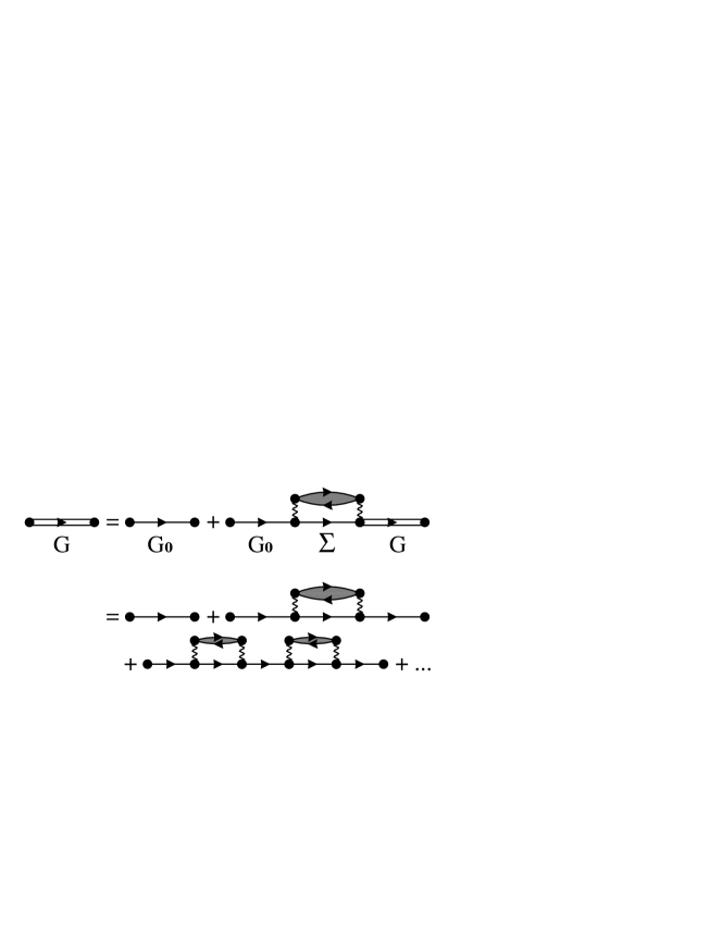
Figure 2: The Feynman diagrams associated with the perturbative expansion of the Dyson equation [Eq. (3) or Eq. (6)].

In our work, we start from the HF Green’s function and RPA response function (together with the residual force $\kappa$) and we obtain the self-energy from Eq. (13). Then, we also solve numerically the Dyson equation in the form (10): for every energy of interest this equation can be cast in matrix form with respect to $r$ and $r^{\prime}$ and solved as

$$G=(1-G_{0}\Sigma)^{-1}G_{0}.$$ (14)

In this way, the perturbed Green’s function $G$ contains the PVC perturbation up to infinite order, in keeping with the fact that it can be expressed by the Feynman diagrams represented in Fig. 2.

II.2 Implementation of the proper treatment of the continuum

II.2.1 Continuum HF Green’s function and continuum RPA response function

As already mentioned, our goal is an implementation of PVC that treats the continuum properly. In the case of atomic nuclei, in particular when local functionals like those based on the Skyrme interaction are used, considerable efforts have been made in this direction as far as the HF-RPA formalism is concerned. Indeed, the Green’s function RPA has been formulated with Skyrme forces, with or without Bertsch1 ; Bertsch2 the continuum; the first self-consistent continuum calculations have been presented in Ref. Liu . In this context, proper treatment of the continuum means that the Schrödinger equation including the HF mean field can be solved at any positive energy with the correct boundary conditions and, based on this, an exact representation of the HF Green’s function $G_{0}$ can be obtained.

This unperturbed HF Green’s function can be written as

$$G_{0,lj}(rr^{\prime};E)=\frac{1}{W(u,v)}u_{lj}(r_{<};E)v_{lj}(r_{>};E),$$ (15)

where $u_{lj}(r;E)$ and $v_{lj}(r;E)$ are, respectively, the regular and irregular solutions of the radial HF equation at energy $E$, $r_{>}$ ($r_{<}$) are the larger (smaller) between $r$ and $r^{\prime}$, and $W(u,v)$ is the Wronskian given by

$$W(u,v;E)=\frac{\hbar^{2}}{2m^{*}(r)}\left(u_{lj}(r;E)\frac{\partial v_{lj}(r;E)}{\partial r}-v_{lj}(r;E)\frac{\partial u_{lj}(r;E)}{\partial r}\right).$$ (16)

$\frac{\hbar^{2}}{2m^{*}(r)}$ is the (radial-dependent) HF effective mass which is defined as usual, in terms of the Skyrme force parameters, as

$$\frac{\hbar^{2}}{2m^{*}_{q}(r)}=\frac{\hbar^{2}}{2m}+\frac{1}{4}\left\{t_{1}\left(1+\frac{1}{2}x_{1}\right)+t_{2}\left(1+\frac{1}{2}x_{2}\right)\right\}\rho(r)-\frac{1}{8}\left\{t_{1}\left(1+2x_{1}\right)+t_{2}\left(1+2x_{2}\right)\right\}\rho_{q}(r).$$ (17)

In order to take properly into account the continuum effects also for the RPA phonons that lie above the threshold, the RPA response function appearing in the self-energy function will be calculated self-consistently, using the same Skyrme Hamiltonian used to compute the mean field. The details of the continuum RPA calculation have been given in previous papers sagawa ; mizuyama . We simply recall that two-body spin orbit and Coulomb terms, as well as spin-dependent terms, are dropped in the residual interaction. It is also necessary to convert the continuum RPA response function into the causal function, because normally the linear response theory (RPA) is formulated in terms of the retarded functions. This point is further discussed in Appendix B.

II.2.2 Contour integration in the complex energy plane.

Formally, the equations that appear in Subsec. II.1 are defined in a model space which does not have an upper bound: in fact, the integrals over energy extend in principle from $-\infty$ to $+\infty$, and single-nucleon as well as phonon energies have only a natural lower bound. However, the self-energy function does not converge if the upper limit on $\omega^{\prime}$ [Eqs. (7) and (13)] is extended to infinity, in keeping with the well-known ultraviolet divergence associated with the zero-range character of Skyrme forces. To avoid this, one must introduce a cutoff $E_{\rm cut}$.

In order to make sure that only states below that cutoff contribute to the integrals in Eq. (7) and (13), one can use the following procedure. By considering the expression (13) for the self-energy function, one notices that the integral receives contribution from the poles of the causal HF Green’s function and the causal RPA response function. The positions of these discrete and continuum (i.e., branch-cut) poles in the complex energy plane are schematically shown in Fig. 3. The blue dots and line represent the poles of the RPA response function, while the black crosses and line represent the poles of the HF Green’s function. In order to pick up correctly the contribution of the poles below the cutoff, we must replace the integral $\int_{-\infty}^{\infty}$ in Eq. (13) by an integral $\int_{C}$ over an appropriate contour path. We have adopted the rectangular integration path displayed in Fig. 3, which is similar to that employed in Ref. matsuo1 . It extends between $-E_{\rm cut}$ to $E_{\rm cut}$ on the real axis, and from 0 to -$\eta^{\prime}$ on the imaginary axis.

It can also be shown that in this way one can reproduce the correct spectral representation of the self-energy function [cf. Eq. (50)] in the limit of a discrete system.

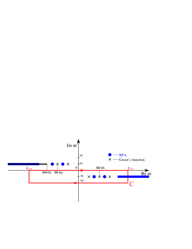
Figure 3: (Color online) Contour path $C$ for the integration on $\omega^{\prime}$ in Eq. (7) and Eq. (13). The blue dots and lines represent the poles of the RPA response function. The black crosses and line represent the poles of the HF Green’s function. For the parameters $\eta$, $\eta^{\prime}$ and $E_{\rm cut}$ see the text.

II.2.3 Single-particle level density

The level density associated with the HF single-particle levels can be defined by using the HF Green’s function $G_{0}$ as

$$\rho_{0,lj}(\omega)=\frac{\pm 1}{\pi}\int_{0}^{R}dr\ \mbox{Im}G_{0,lj}(rr,\omega),$$ (18)

where $R$ is the upper limit of the integration. For bound states at negative energies, one is guaranteed that the result is stable with respect to increasing $R$. The sign $\pm$ guarantees that the level density is positive, i.e., the sign +(-) refers to particle (hole) states. This is equivalent to the definition $\rho_{0,lj}(\omega)=\sum_{n}\delta(\omega-e^{0}_{nlj})$ and is normalized to 1 for bound states. In the absence of any potential, $\rho_{0,lj}(\omega)$ reduces to the free particle level density $\rho_{free,lj}(\omega)$, obtained by replacing $G_{0,lj}$ with the Green’s function for the free particle which satisfies $(\omega-\frac{p^{2}}{2m})G_{free}=1$. $G_{free}$ can be calculated either numerically or analytically using the same definition of Eq. (15), but with the use of the wave function for the free particle. This free particle level density is $\rho_{free,lj}(\omega)\propto\sqrt{\frac{2m}{\hbar^{2}}}\frac{R}{2\pi\sqrt{\omega}}$ for large value of $\omega$. For $R\to\infty$, $\rho_{free,lj}$ diverges. On the other hand, $\rho_{0,lj}(\omega)$ tends to $\rho_{free,lj}$ for large values of $\omega$. It is then useful to introduce a new level density $\bar{\rho}_{0,lj}(\omega)$ by subtracting $\rho_{free,lj}(\omega)$ shlomo , that is,

$$\bar{\rho}_{0,lj}(\omega)=\frac{\pm 1}{\pi}\int_{0}^{R}dr\ \mbox{Im}\left(G_{0,lj}(rr,\omega)-G_{Free,lj}(rr,\omega).\right)$$ (19)

In this way, the dependence on $R$ is eliminated also for positive energies (cf. Fig. 5). For $\omega<0$, there is no contribution associated with the free particles. As mentioned above, $\bar{\rho}_{0,lj}$ coincides with the usual definition of the level density for the single-particle levels shlomo

$$\bar{\rho}_{0,lj}(\omega)=\left\{\begin{array}[]{ll}\displaystyle{\sum_{n}\delta(\omega-\epsilon^{(0)}_{nlj})}&\mbox{for bound states\ }(\omega<0),\\ \displaystyle{\frac{1}{\pi}\frac{d\delta^{(0)}_{lj}}{d\omega}}&\mbox{for positive energy states\ }(\omega>0).\end{array}\right.$$ (22)

In an analogous way, we define the perturbed (HF+PVC) level density by using the solution of the Dyson equation $G_{lj}$ as

$$\bar{\rho}_{lj}(\omega)=\frac{\pm 1}{\pi}\int dr\ \mbox{Im}\left(G_{lj}(rr,\omega)-G_{Free,lj}(rr,\omega)\right)$$ (23)

The peaks of the perturbed level density provide renormalized single-particle energies which include the effect of the particle-phonon coupling. In fact, if this coupling is small one can expect a simple shift of the HF peaks. Otherwise, the s.p. strength can be quite fragmented: the associated widths reflect the basic decay mechanisms that are the nucleon decay (providing the so-called escape width, or $\Gamma^{\uparrow}$) and the spreading into the complicated configurations made up with nucleons and vibrations (providing the spreading width $\Gamma^{\downarrow}$).

III Results

We shall present results for three nuclei: ⁴⁰Ca, ²⁰⁸Pb and ²⁴O. The effective Skyrme interaction SLy5 Chabanat is used to calculate the HF mean field. The calculation of the RPA response is carried out exactly as described in Ref. mizuyama in the limit of no pairing, using all the terms of the SLy5 interaction, except for the two-body spin-dependent terms, the spin-orbit terms and the Coulomb term in the residual p-h force. In the calculations, the angular momentum cutoff for the unoccupied continuum states is set at $l_{cut}=7\hbar$ for ⁴⁰Ca, and $l_{cut}=12\hbar$ for ²⁴O and ²⁰⁸Pb, respectively. The radial mesh size is $\Delta r=0.2$ fm. The values of the parameters used in the contour integrations (see the discussion in II.2.2) are $\eta=$ 0.2 MeV [cf. Eq. (13)] and $\eta^{\prime}=2\eta$ [cf. Eq. (10)].

There are a few important issues that we wish to stress:

1. Due specifically to the zero-range character of the Skyrme interaction, the self-energy diverges logarithmically as a function of the maximum energy of the phonons, as it has mentioned above. The first steps towards a systematic renormalization procedure have only recently been started to be worked out colodiverg . In this work, we shall take the usual view that the important couplings are those associated with the collective low-lying states and giant resonances. We shall then include phonons associated with the multipolarities $2^{+}$, $3^{-}$, $4^{+}$ and $5^{-}$, and set an upper cutoff on the phonon energies given by $E_{\rm cut}=60$ MeV because no strong peaks are present above this value in the calculated RPA strengths. The way in which this cutoff is implemented has been described in detail in II.2.2.

2. In the present scheme, the price to be paid for the exact continuum treatment, is that one cannot discriminate between the inclusion of collective and non-collective phonons. Actually, the diagrams shown in Figs. 1 and 2 contain terms that violate the Pauli principle, and these terms are larger when the phonons are non-collective. In other words, one could expect that in an exact calculation the correction of the Pauli principle violation cancels, to a large extent, the contributions from non-collective phonons. Although this point has never been clarified in the available literature, to our knowledge, on a quantitative basis, in most of the cases the usual view has been to take into account only the coupling to collective states. In the work that we quoted already (the most similar to the present one), namely in the recent calculation of particle-vibration coupling in ⁴⁰Ca and ²⁰⁸Pb of Ref. colo10 , only phonons exhausting at least 5% of the isoscalar or isovector non-energy-weighted sum rules have been taken into account. Therefore, we can expect that the effect of particle-vibration coupling is larger when we calculate it with the present method, as compared with Ref. colo10 . We shall come back to this issue below.

3. The momentum-dependent part of the particle-hole interaction had previously been neglected in the calculation of the particle-vibration coupling; then, in Ref. colo10 it was shown that its effect is important (at least in the case of the SLy5 interaction), and that it can be reasonably accounted for within the Landau-Migdal (LM) approximation, by choosing the Fermi momentum $k_{F}$ as 1.33 fm^-1 (that is, at the value associated with the nuclear matter saturation density). The LM approximation will be adopted in the following, with the same value of $k_{F}$.

III.1 Results for ⁴⁰Ca

The first essential steps of our work consist in the calculation of the HF spectrum and of the RPA strength functions. The results are illustrated respectively in Table 1 (HF single-particle spectrum) and in Fig. 4 (isoscalar and isovector RPA strength functions associated with the multipolarities $2^{+},3^{-},4^{+}$ and $5^{-}$). In Table 2 we give the theoretical energies and transition strengths for the low-lying collective $3^{-}$ and $5^{-}$ states, comparing them with available data.

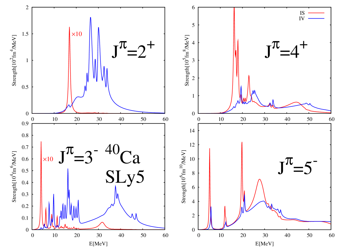
Figure 4: (Color online) Isoscalar (IS) and isovector (IV) RPA strength functions in ⁴⁰Ca for the multipolarities $2^{+},3^{-},4^{+}$ and $5^{-}$. The IS $2^{+}$ and IS $3^{-}$ strength functions are reduced by a factor 10.

Nucleus	hole states [MeV]		particle states [MeV]
40Ca	$1s\frac{1}{2}$	-48.3	$1f\frac{7}{2}$	-9.7
	$1p\frac{3}{2}$	-35.0	$2p\frac{3}{2}$	-5.3
	$1p\frac{1}{2}$	-31.0	$2p\frac{1}{2}$	-3.1
	$1d\frac{5}{2}$	-22.1	$1f\frac{5}{2}$	-1.3
	$2s\frac{1}{2}$	-17.3
	$1d\frac{3}{2}$	-15.2

Table 1: Neutron single-particle energies in ⁴⁰Ca.

		Theory (RPA)			Experiment
Nucleus	$J^{\pi}$	Energy	$B(Q^{\tau=0}_{J})$		Energy	$B(Q^{\tau=0}_{J})$
		[MeV]	[e2fm2J]		[MeV]	[e2fm2J]
40Ca	$3^{-}$	4.13	$1.13\times 10^{4}$		3.74	$1.84\times 10^{4}$
	$5^{-}$	5.25	$2.22\times 10^{6}$		4.49	–

Table 2: The theoretical values for the energy and the transition strength $B$ of the low-lying isoscalar $3^{-}$ and $5^{-}$ states in ⁴⁰Ca are compared with the experimental data, that are taken in the case of the $3^{-}$ state from Ref. nucltableBE3 and in the case of the $5^{-}$ state from Ref. nucldata102 .

In Fig. 5 we compare the level densities $\rho_{0,lj}$, $\rho_{Free,lj}$ and $\bar{\rho}_{0,lj}$ defined above [cf. Eqs. (18-23)], in case of neutrons and for the quantum number g_9/2. The results are shown for different values of the upper limit of integration, namely $R$ = 15, 20 and 25 fm. The main goal of the figure is to illustrate the effect of the removal of the free particle level density, that has been formally introduced above (cf. II.2.3). In fact, it can be seen in panels (a) and (b) that for each value of $R$ the smooth tails of $\rho_{Free,lj}(\omega)$ and $\rho_{0,lj}$ converge, for $\omega$ between 5 and 10 MeV, towards the asymptotic value $\sqrt{\frac{2m}{\hbar^{2}}}\frac{R}{2\pi\sqrt{\omega}}$ indicated by the dashed lines and by the symbol $f(R,\omega)$ in the panels. In panel (c) we show the level density $\bar{\rho}_{0,lj}(\omega)$ defined by Eq. (19). The free level density is eliminated (and the dependence on $R$ with it) so that one can clearly identify the pure g_9/2 resonance in the continuum. The inclusion of PVC leads to a quite big fragmentation of the strength, as it can be seen in panels (d) and (e) of Fig. 5: panel (d) is meant to mainly show that the 3^- states are the most important to produce that fragmentation, whereas in panel (e) we illustrate the effect of the subtraction procedure on the perturbed level density.

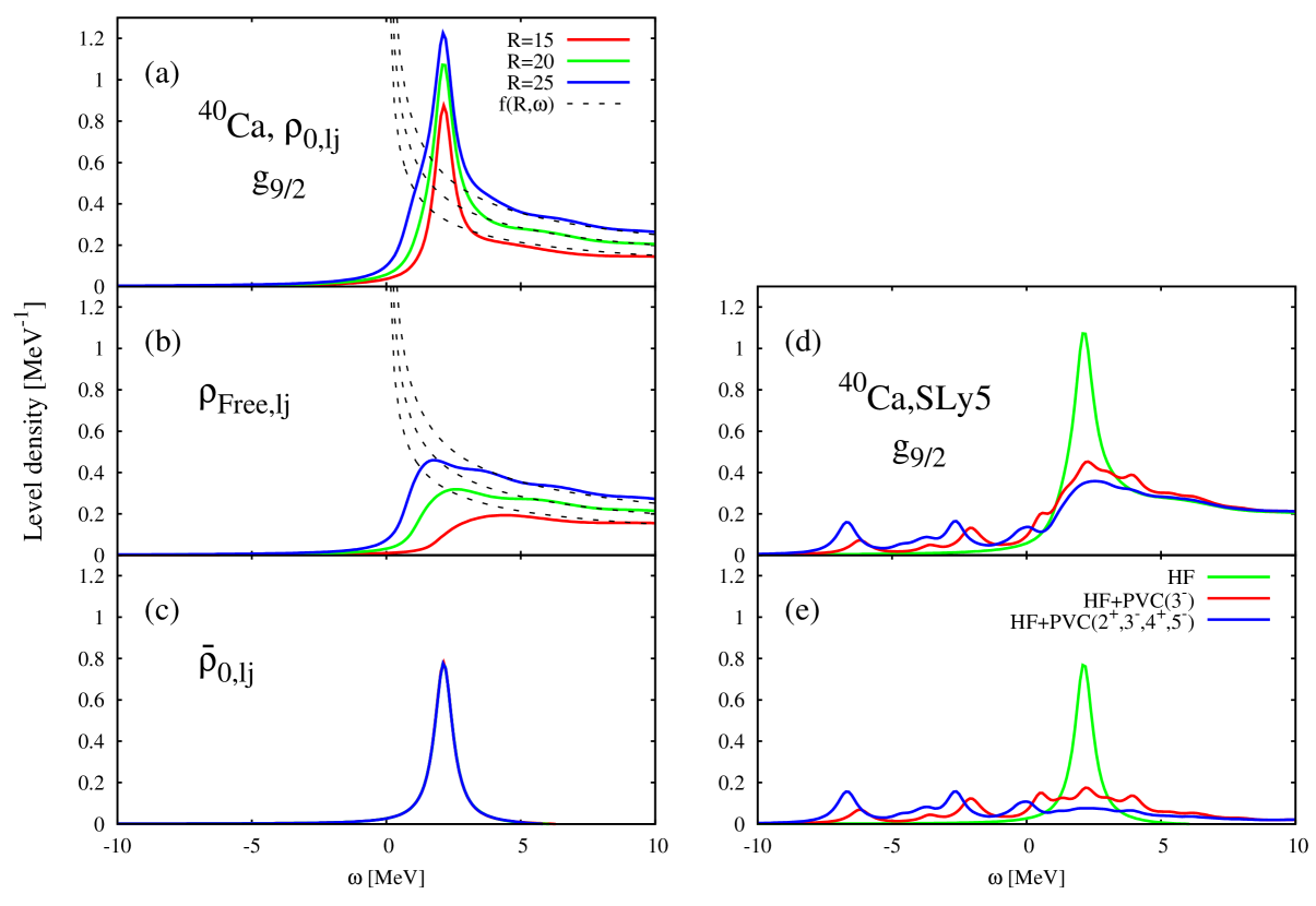
Figure 5: (Color online) Neutron level density in the case of the g_9/2 quantum numbers for ⁴⁰Ca. These quantum numbers are associated with a single-particle resonance in the HF mean field. In panels (a), (b) and (c) we show respectively the quantities $\rho_{0,lj}$, $\rho_{Free,lj}$, and $\bar{\rho}_{0,lj}$ defined in Eqs. (18-23), for three different values of the upper integration limit $R$, namely 15 fm (red curve), 20 fm (green curve) and 25 fm (blue curve). The asymptotic expression for the free particle level density, $f(R,\omega)=\sqrt{\frac{2m}{\hbar^{2}}}\frac{R}{2\pi\sqrt{\omega}}$ is shown in (a) and (b). Note that in (c) the curves corresponding to different values of $R$ practically coincide, because the free particle contribution is removed from $\bar{\rho}_{0,lj}$. In (d) we show the perturbed densities ${\rho}_{lj}$, obtained by solving the Dyson equation with the inclusion of the coupling either with all multipolarities (blue curve) or with only the $3^{-}$ (red curve). They are compared with the HF density $\rho_{0,lj}$ (green curve, $R$=20 fm) already shown in (a). In (e) we show the corresponding perturbed densities $\bar{\rho}_{lj}$, obtained by subtracting the free-particle level density. They are compared with the HF density $\bar{\rho}_{0,lj}$ already shown in (c).

Since the parameter $\eta$ introduced in our definition of Green’s functions and response functions is one of the numerical inputs of our calculations, we have carefully checked whether the results are sensitive to the choice of its value. In Fig. 6, we compare the densities $\bar{\rho}_{lj}$ obtained with our standard choice of the the smearing parameter $\eta$ = 0.2 MeV, and with $\eta$ = 0.1 MeV, again corresponding to ⁴⁰Ca and the Skyrme set SLy5, in the case of the quantum numbers g_9/2 and p_1/2. It is quite reassuring that the structure displayed by the peaks of the level density does not depend on the chosen value of $\eta$. In principle, we may expect that a dependence of this kind shows up in the discrete part of the spectrum and vanishes when the continuum coupling becomes dominant: this effect can be to some extent seen in the high-energy part (above $\approx$ 5 MeV) of the upper panel of the figure.

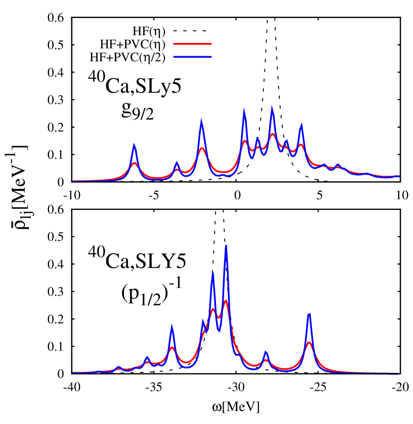
Figure 6: (Color online) Dependence of the HF+PVC level density $\bar{\rho}_{lj}$ [cf. Eq. (23)] on the smearing parameter $\eta$, for the g_9/2 states (upper panel) and for the p_1/2 states (lower panel). Only the coupling with $3^{-}$ phonons is taken the account. The red curves show the results obtained with the standard value $\eta=0.2$ MeV, while the blue curves have been obtained with $\eta=$ 0.1 MeV. We also show the HF results (dashed curves, obtained with $\eta=$ 0.2 MeV).

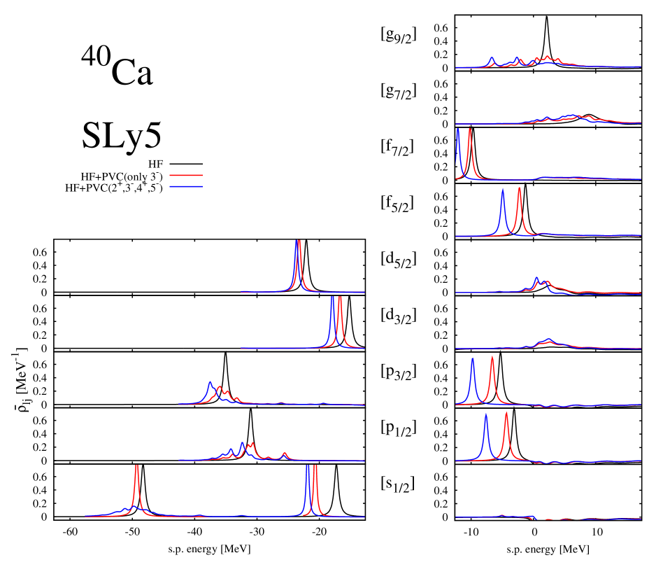
Figure 7: (Color online) The single particle level density $\bar{\rho_{lj}}$ for neutron states in ⁴⁰Ca defined by Eq. (19) for HF and Eq. (23) for HF+PVC. The left panel refers to hole states, the right panel to particle states. The black curve represents the HF level density, while the red curve and the blue curve show level densities resulting from the coupling to phonons. In the case of the red curve, only $3^{-}$ RPA phonons are taken into account, while in the case of the blue curve $2^{+},3^{-},4^{+}$ and $5^{-}$ phonons are taken into account.

In Fig. 7, we show results for the single-particle level density $\bar{\rho}_{lj}$ in ⁴⁰Ca, associated with various quantum numbers. The unperturbed level density is shown by means of the black curve, and displays sharp peaks of equal heights at the HF energies. We compare in the figure the results obtained by taking into account the coupling with all multipolarities (blue curve), or with $3^{-}$ phonons only (red curve). The first qualitative remark is that for the states lying close to the Fermi energy, both in the case of hole states (2s_1/2, 1d_5/2 and 1d_3/2) and bound particle states (2p_3/2, 2p_1/2, 1f_7/2 and 1f_5/2), the strength remains concentrated in a single peak, eventually acquiring a spectroscopic factor, and the quasiparticle picture maintains its validity. This is not true when we consider states either more far from the Fermi surface or in the continuum, that is, at energies where we expect the single-particle self-energy to become larger.

The hole states are in the left part of Fig. 7. For the aforementioned 2s and 1d states there is only a shift of the HF peak. Instead, in the case of 1p_1/2 and 1p_3/2 states the strength is damped over a broad interval. It is interesting to trace the origin of this fragmentation, by restricting the summation over the phonon multipolarity and the angular momentum of the intermediate single-particle states in Eq. (13), and analyzing the contribution of specific configurations.

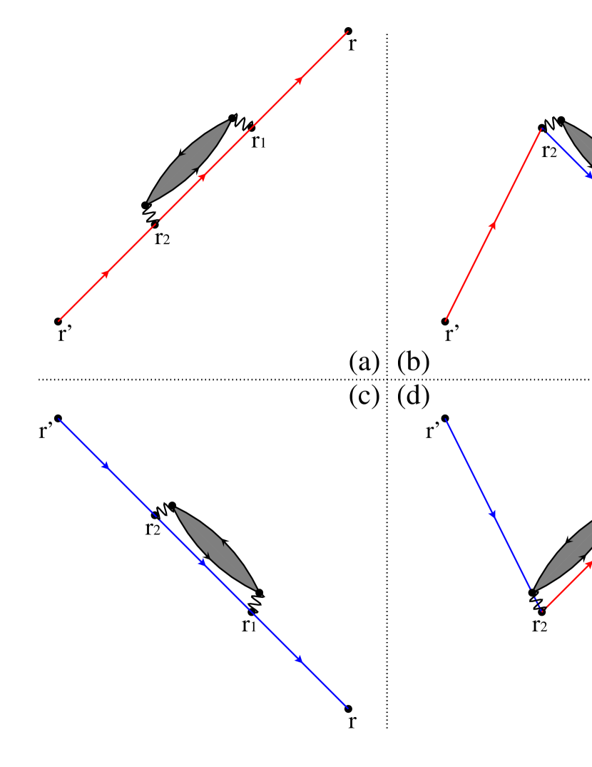
Figure 8: (Color online) Feynman diagrams associated with particle [(a) and (b)] and hole [(c) and (d)] states. The shaded area denotes the RPA phonon and the wavy lines correspond to the interaction. See the text for further discussion.

To help the following discussion, we depict in Fig. 8 selected contributions to the particle [(a) and (b)] and hole [(c) and (d)] self-energy. Since our equations and numerical codes are written in the coordinate space, these different contributions cannot, strictly speaking, be singled out. However, at definite energies it may happen that only one is dominant. We use Fig. 8 to recall that the fragmentation of a hole state can only be caused by on-shell contributions associated with the coupling with other hole-phonon configurations [panel (c)], while the coupling with particle states [panel (d)] can only produce an energy shift.

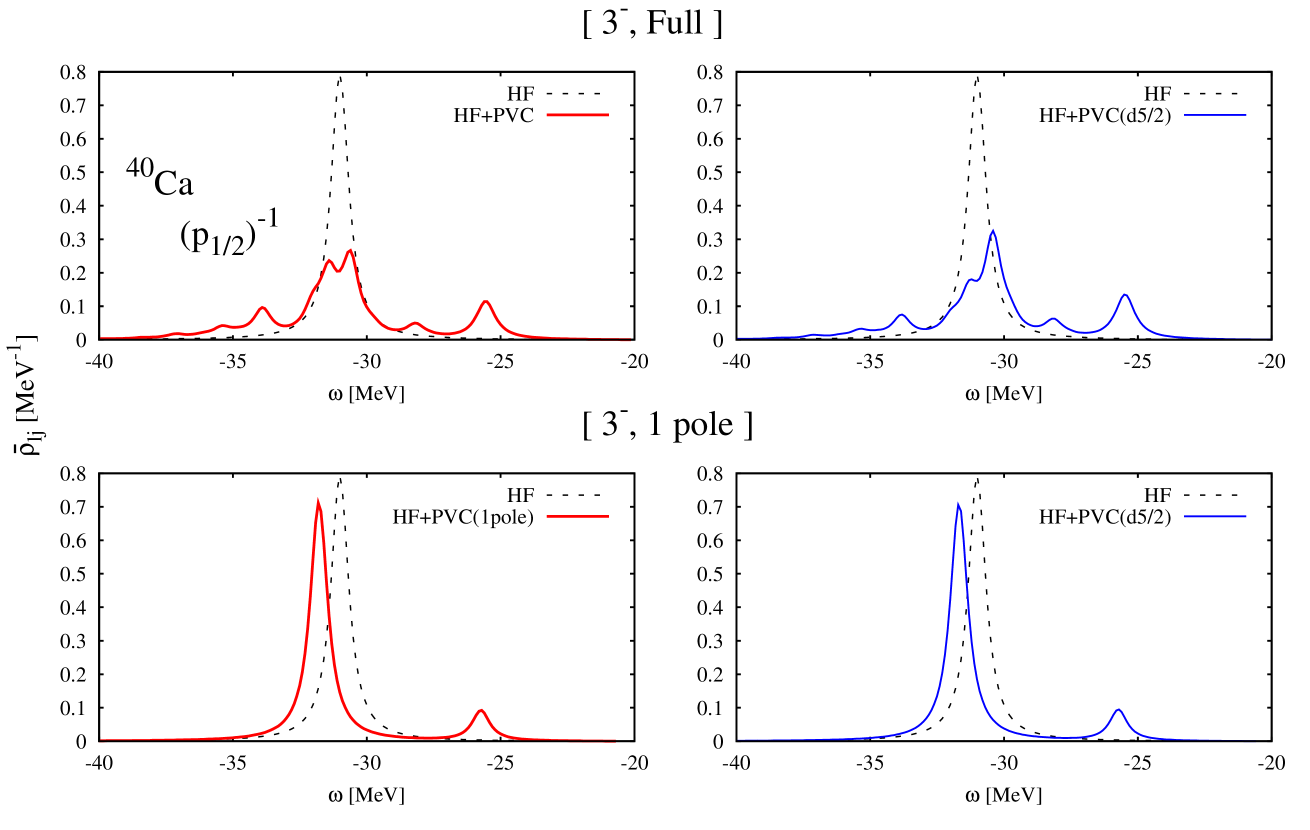
Figure 9: (Color online) Analysis of the (p_1/2)^-1 level density in ⁴⁰Ca produced by the coupling with $3^{-}$ phonons. In the upper panels, all the calculated RPA $3^{-}$ phonons are included in the calculation. In the lower panels, only the lowest $3_{1}^{-}$ phonon state is instead taken into account. In the left panels, all possible intermediate single-particle configurations are included. In the right panel, the intermediate configurations are restricted to d${}_{5/2}\otimes 3^{-}$.

The unperturbed (s_1/2)^-1 strength shows two peaks, associated with the 1s_1/2 ($e_{1\rm s1/2}\approx-50$ MeV) and 2s_1/2 ($e_{2\rm s1/2}\approx-20$ MeV) single-particle states. Due to parity and angular momentum conservation, the only intermediate hole-phonon configurations s_1/2 holes can couple to are (d_3/2)${}^{-1}\otimes 2^{+}$ and (d_5/2)${}^{-1}\otimes 2^{+}$. These coupling can lead to a strong fragmentation of the (1s_1/2)^-1 strength. In fact, the energy differences $e_{1\rm d3/2}-e_{1\rm s1/2}=-15.2+48.3=33.1$ MeV and $e_{1\rm d5/2}-e_{1\rm s1/2}=-22.1+48.3=26.2$ MeV (cf. Table 1) are close to the centroid of the isovector quadrupole strength ($E_{\rm IVGDR}=29.2$ MeV, cf. Fig. 4). On the other hand, although the (1$d_{3/2}$)${}^{-1}\otimes 2^{+}$ intermediate configuration could in principle contribute to the fragmentation of the (2s_1/2)^-1 state, in this case the energy difference is low, namely $e_{1\rm d3/2}-e_{1\rm s1/2}=-15.2+17.3=2.1$ MeV. In ⁴⁰Ca there is no low-lying quadrupole strength, and therefore the HF strength is shifted but not fragmented. In a similar way, one concludes that the d_3/2 and d_5/2 hole strength, that lies close to the Fermi energy, cannot be fragmented. The deeply bound p_1/2 and p_3/2 states can instead couple efficiently, respectively to the (1d_5/2)${}^{-1}\otimes 3^{-}$ and to the (1d_3/2)${}^{-1}\otimes 3^{-}$ configurations. The relevant energy differences lie in the range $9\sim 20$ MeV, where one finds substantial $3^{-}$ strength (cf. Fig. 4). The case of $p_{1/2}$ is analyzed in more detail in Fig. 9, including only $3^{-}$ phonons. It is seen that the full calculation (top panel, left) is very similar to the result obtained including only (1d${}_{5/2})^{-1}\otimes 3^{-}$ configurations (top panel, right). Coupling only to the lowest phonons of each multipolarity (bottom panel, left) leads only to a modest energy shift, again caused essentially by the (1d_5/2)${}^{-1}\otimes 3_{1}^{-}$ configuration (bottom panel, right). The remnant of this configuration is visible in the figures, at about -25 MeV.

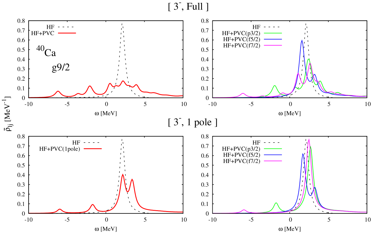
Figure 10: (Color online) The same as Fig. 9 in the case of the g_9/2 level density. In the right panel, we show results obtained by taking into account only the coupling to specific intermediate configurations: p${}_{3/2}\otimes 3^{-}$ (green curve), f${}_{5/2}\otimes 3^{-}$ (blue curve), and f${}_{7/2}\otimes 3^{-}$ (purple curve), respectively.

The results obtained for the particle states are depicted in the right part of Fig. 7. As already mentioned, those lying close to the Fermi energy (2p_3/2, 2p_1/2, 1f_7/2 and 1f_5/2) can be well described within the quasiparticle picture: the associated single-particle strength shows a well defined peak, which is shifted from the unperturbed (HF) position. The situation is quite different for the unbound particle states 1g_7/2 and 1g_9/2 which are strongly fragmented. For these states, we expect that our proper treatment of the continuum should be particularly important. The case of the 1g_9/2 orbital, which in the HF calculation is associated with a low-lying resonance lying at about 2.5 MeV, is analyzed in more detail in Fig. 10. We consider only the coupling with $3^{-}$ phonons, since they produce most of the fragmentation. By comparing the left and the right top panels of Fig. 10, one concludes that the strong fragmentation of the resonant level is caused by the coupling with several intermediate configurations [namely (p_3/2)$\otimes 3^{-}$, (f_5/2)$\otimes 3^{-}$ and (f_7/2)$\otimes 3^{-}$]. The two satellite peaks found at $\approx-6$ MeV and at $\approx-2$ MeV are produced by specific configurations, associated with the lowest $3^{-}_{1}$ collective state (cf. bottom panel, right). This phonon is responsible for about half of the total width (compare bottom panel, left with top panel, left).

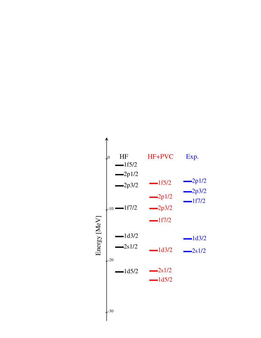
Figure 11: (Color online) Energy of the seven neutron bound states lying close to the Fermi energy in ⁴⁰Ca, calculated in HF (left) and by taking into account the coupling to phonons (right).

In Fig. 11 we compare the position of the seven HF energy levels lying close to the Fermi energy with the position of the shifted levels, deduced from Fig. 7. Only for these levels a centroid energy is quite meaningful because, as we have already emphasized, for these levels essentially only one peak exists when one looks at the PVC results and the quasiparticle picture holds. Also for these levels, and for them only, one can attempt a comparison with the results of Ref. colo10 that have been obtained through second-order perturbation theory and in a very similar scheme. The results are in overall agreement with those of Ref. colo10 , although the magnitude of the present energy shifts is larger. In fact, while in Ref. colo10 the shifts are typically between -1 and -2 MeV, here they range between -1.5 and -4.5 MeV. We attribute this difference mainly to the coupling with non collective phonons. As it was discussed alreday in Ref. colo10 , the energy shifts are mostly due to coupling with intermediate configurations including an octupole phonon. If we compare the theoretical results with experiment, we must probably conclude that a re-fitting of the effective force (SLy5 in the present case) is needed if this has to be used outside the mean-field framework. In fact, the HF-PVC results need a global upward shift in energy.

III.1.1 Comparison with the experimental data in ⁴⁰Ca

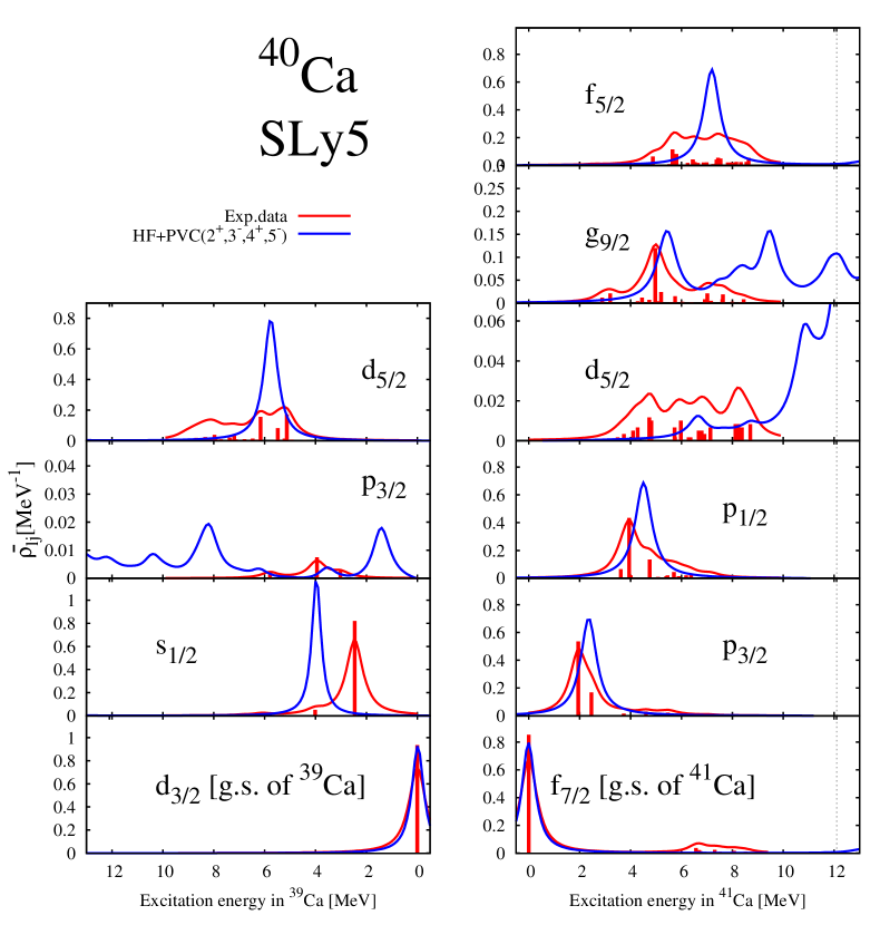
Figure 12: (Color online) The theoretical level densities $\bar{\rho_{lj}}$ (blue curves) are shown as a function of the excitation energy in ³⁹Ca (hole states, left panels) and in ⁴¹Ca (particle states, right panels). Except for the change of scale, the results are the same already shown in Fig. 7. They are compared with the experimental spectroscopic factors taken from nucldataA39 ; nucldataA41 : these are represented in histogram form and also convoluted with Lorentzian functions of width 0.4 MeV (red curve). The vertical dotted line shows the one-neutron theoretical threshold energy obtained within HF+PVC (this energy is then the continuum threshold measured by setting at zero the energy of the renormalized 1f_7/2 state already displayed in Figs. 7 and 11).

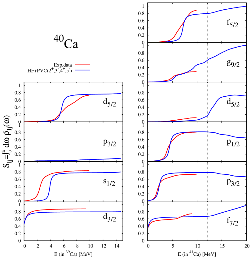
Figure 13: (Color online) The integrated level density as a function of excitation energy for ³⁹Ca (left panel) and ⁴¹Ca (right panel), respectively. The red curves correspond to the experimental data, while the blue curves are our HF+PVC calculation.

40Ca
Holes				Particles
	$S_{lj}(^{39}$Ca)				$S_{lj}(^{41}$Ca)
$J^{\pi}$	Exp.	Theory		$J^{\pi}$	Exp.	Theory
d3/2	0.88	0.80		f7/2	0.74	0.66
s1/2	0.84	0.80		p1/2	0.80	0.81
p3/2	$2.9\times 10^{-3}$	0.05		p3/2	0.73	0.79
d5/2	0.73	0.75		d5/2	0.11	0.04
				f5/2	0.88	0.77
				g9/2	0.28	0.36

Table 3: Experimental spectroscopic factors $S_{lj}$ obtained from one-nucleon transfer reactions for hole and particle states in ³⁹Ca and ⁴¹Ca, compared to the integral of the theoretical level density performed up to an excitation energy of 10 MeV (cf. Fig. 13).

The experimental single-particle strength of ⁴⁰Ca is obtained from ${}^{40}\mbox{Ca}(\rm p,\rm d)^{39}\rm Ca$ pickup (for hole states) and ${}^{40}\mbox{Ca}(\rm d,\rm p)^{41}\rm Ca$ stripping reactions (for particle states), by comparing the measured cross sections with Distorted Wave Born Approximation (DWBA) calculations performed with conventional assumptions. In particular, one usually assumes that the wavefunction of the transferred nucleon, $\phi_{nlj}$ can be taken as an eigenfunction of a static mean field potential, by adjusting the depth of that potential so that the binding energy becomes equal to the experimental separation energy and the correct asymptotic dependence is guaranteed. The comparison with the level density obtained in a calculation like the present one, although not straightforward, is reasonable for levels which are well described by the one-quasiparticle approximation. In the previous subsection, we have seen that this is indeed the case for several states close to the Fermi energy: for them, the single-peak associated with a definite value of the number of nodes $n$, appearing in HF, persists. A diagonal, even perturbative, approximation for the mass operator is quite appropriate. However, for states characterized by a broad distribution in energy, when several values of $n$ are mixed, the comparison with a simple DWBA calculation is likely to be less reliable (cf., e.g., the discussion in Ref. Satchler ). In principle, one should rather perform a direct theoretical calculation of the transfer cross section, using the wavefunctions that include many-body correlations. This goes beyond the scope of the current paper, and in the following we shall limit ourselves to a simple comparison with the spectroscopic factors reported in the experimental papers nucldataA39 ; nucldataA41 . Our results are comparable to those obtained in Ref. eckle , where the distribution of single-particle strength in ⁴⁰Ca was calculated in a (discrete) quasiparticle-coupling model going beyond the diagonal approximation. The red histogram bars in Fig. 12 show the experimentally determined spectroscopic factors, which are convoluted with Lorentzian functions having a width equal to 0.4 MeV to produce the red continuous lines. These can be compared with our theoretical level densities (blue continuous lines). The dotted vertical line shows the calculated threshold for one-neutron emission, which overestimates the experimental value by about 2 MeV.

The total single-particle strength associated with the different quantum numbers ${l,j}$, obtained by integrating the level densities displayed in Fig. 12 up to $\rm E=10$ MeV is reported in Table 3. One finds an overall satisfactory agreement between theory and experiment. The position of the centroid energies is reasonably well reproduced, except that in the case of the s_1/2 strength, where the theoretical centroid energy is too low by about 2 MeV. In general, theory tends still to underestimate the fragmentation of the single-particle strength: this occurs in particular for the d_5/2 strength (for particles and holes), and for the f_5/2 strength (for particles). This can be seen also from Fig. 13, where we show the cumulated experimental and theoretical strength distributions. The latter distributions tend to show a sharper increase. This can be attributed to several reasons. Among the possible ones, we point out that the present RPA calculation underestimates the experimental value of the collectivity of the low-lying 3${}^{-}_{1}$ phonon (cf. Table 2) and cannnot describe in detail the ISGQR strength distribution. If one could include its admixture with two particle-two hole configurations, these could shift part of the strength at lower energy and increase the effect of the coupling with the single-particle strength. A more fragmented ISGQR distribution would be in better agreement with experiment Kamer ; Harakeh ; however, such a calculation would require to go beyond the formalism of the present work.

III.2 Results for ²⁰⁸Pb

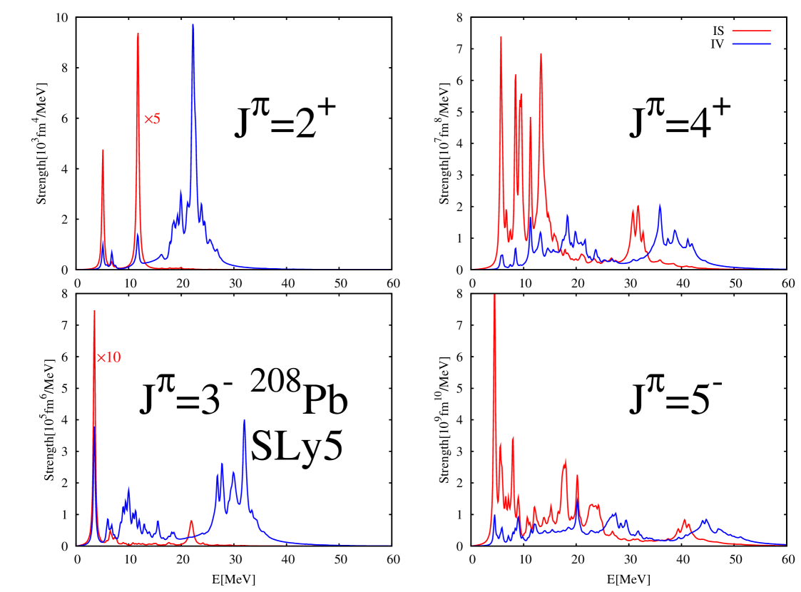
Figure 14: (Color online) The RPA strength functions in ²⁰⁸Pb obtained from our RPA calculations. The IS $2^{+}$ strength is reduced by a factor 5, while the IS $3^{-}$ strength is reduced by a factor 10.

		Theory (RPA)			Experiment
Nucleus	$J^{\pi}$	Energy	$B(Q^{\tau=0}_{J})$		Energy	$B(Q^{\tau=0}_{J})$
		[MeV]	[e2fm2J]		[MeV]	[e2fm2J]
208Pb	$2^{+}$	5.12	$2.35\times 10^{3}$		4.09	$3.00\times 10^{3}$
	$3^{-}$	3.49	$7.08\times 10^{5}$		2.62	$6.11\times 10^{5}$
	$4^{+}$	5.69	$5.16\times 10^{6}$		4.32	$15.5\times 10^{6}$
	$5^{-}$	4.49	$4.96\times 10^{8}$		3.20	$4.47\times 10^{8}$

Table 4: Energies and electromagnetic transition probabilities associated with the low-lying isoscalar collective states in ²⁰⁸Pb. The experimental data are taken from Refs. nucltableBE2 ; nucltableBE3 .

In Fig. 14 we provide an overall view of the calculated RPA multipole strength in ²⁰⁸Pb, while the energy and transition strength of the lowest states of each multipolarity are reported in Table 4. The properties of the low-lying states are reproduced reasonably well by our calculation, with the partial exception of the transition probability associated with the 4⁺ state. In Fig. 15, we show the results of our systematic calculation of the level densities, displaying the outcome of the full HF+PVC calculation including 2⁺, 3^-, 4⁺ and 5^- phonons (blue curve), as well as the results obtained by including only the 3^- phonons (red curve), in comparison with the HF results (black curve).

Nucleus	Hole states [MeV]		Particle states [MeV]
208Pb	$1\rm s\frac{1}{2}$	-58.0	$4\rm s\frac{1}{2}$	-0.1
	$2\rm s\frac{1}{2}$	-40.6	$3\rm d\frac{5}{2}$	-0.7
	$3\rm s\frac{1}{2}$	-18.8	$2\rm g\frac{9}{2}$	-3.2
	$1\rm p\frac{1}{2}$	-51.2	$1\rm i\frac{11}{2}$	-1.9
	$2\rm p\frac{1}{2}$	-29.8	$1\rm j\frac{15}{2}$	-0.4
	$3\rm p\frac{1}{2}$	-8.1
	$1\rm p\frac{3}{2}$	-51.8
	$2\rm p\frac{3}{2}$	-30.9
	$3\rm p\frac{3}{2}$	-9.2
	$1\rm d\frac{3}{2}$	-43.1
	$2\rm d\frac{3}{2}$	-19.2
	$1\rm d\frac{5}{2}$	-44.5
	$2\rm d\frac{5}{2}$	-21.3
	$1\rm f\frac{5}{2}$	-33.8
	$2\rm f\frac{5}{2}$	-9.1
	$1\rm f\frac{7}{2}$	-36.3
	$2\rm f\frac{7}{2}$	-12.1
	$1\rm g\frac{7}{2}$	-23.5
	$1\rm g\frac{9}{2}$	-27.5
	$1\rm h\frac{9}{2}$	-12.8
	$1\rm h\frac{11}{2}$	-18.5
	$1\rm j\frac{13}{2}$	-9.4

Table 5: Skyrme Hartree-Fock single-particle energies for ²⁰⁸Pb obtained with the force SLy5. Only states at negative energy are reported in the Table.

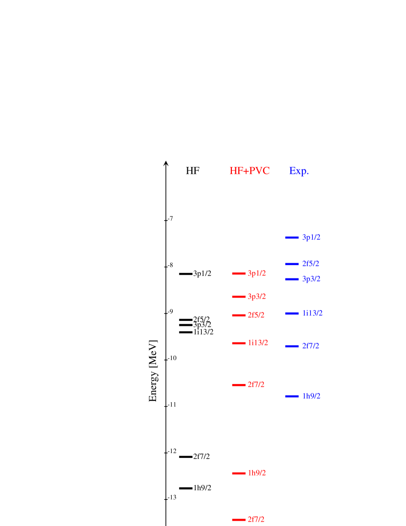
Figure 17: (Color online) Neutron hole states in ²⁰⁸Pb.

The HF single-particle spectrum calculated for ²⁰⁸Pb is reported in Table 5 and illustrated in the left column of Fig. 17 and Fig. 17. In the central column of Fig. 17 and Fig. 17 we show the position of the main peaks obtained from the full HF+PVC calculation, whereas in the right column we include the experimental results. From an overall look at Fig. 15, we can notice that the quasiparticle picture (a single peak emerging from the PVC calculation, with shifted energy and renormalized integral with respect to HF) holds for most of the valence hole states, that is, for 3p_1/2, 2f_5/2, 3p_3/2, 1i_13/2 and 1h_9/2. A partial exception is constituted by the state 2f_7/2, that acquires a double structure mainly due to the coupling with the 3${}^{-}_{1}\otimes\rm i_{13/2}$ configuration. The inclusion of PVC brings the relative position of the valence hole states in much better agreement with experiment. For particle states, the quasi-particle picture seems to be valid for 2g_9/2, 1i_11/2, 3d_5/2, 4s_1/2, 2g_7/2, 3d_3/2 and, only to some extent, for 1j_15/2. The position of the 2g_9/2, 1i_11/2 and 1j_15/2 states is in good agreement with experiment, while the 3d_5/2, 1j_15/2 and 2g_7/2 orbitals lie too high in energy.

The present calculation is similar to the one of Ref. colo10 but the energy shifts are larger, as in the case of ⁴⁰Ca, due probably to the contribution of non-collective states. We can also make an overall comparison with the various results reported in Ref. CM , by evaluating an average particle-hole gap defined as

$$\Delta\omega=\langle\epsilon_{p}\rangle-\langle\epsilon_{h}\rangle,$$ (24)

with

$$\langle\epsilon_{p}\rangle = \frac{\sum_{\rm unocc}(2j+1)\epsilon_{nlj}}{\sum_{\rm unocc}(2j+1)},$$

$$\langle\epsilon_{h}\rangle = \frac{\sum_{\rm occ}(2j+1)\epsilon_{nlj}}{\sum_{\rm occ}(2j+1)},$$ (25)

where the labels “unocc” and “occ” refer to the unoccupied and occupied valence shell, respectively. Starting from the HF value, 9.34 MeV, the HF-PVC value is reduced to 7.89 MeV and gets closer to the experimental value of 6.52 MeV; the difference between the two values, namely -1.45 MeV, compares well with the values presented in Ref. CM , that range between -3.2 MeV and -1.1 MeV.

The processes leading to the fragmentation of the single-particle strength for the orbitals lying far from the Fermi energy in ²⁰⁸Pb have been already extensively discussed within the framework of more phenomenological studies CM ; however, for the convenience of the reader, in the following we present some details of the present calculation.

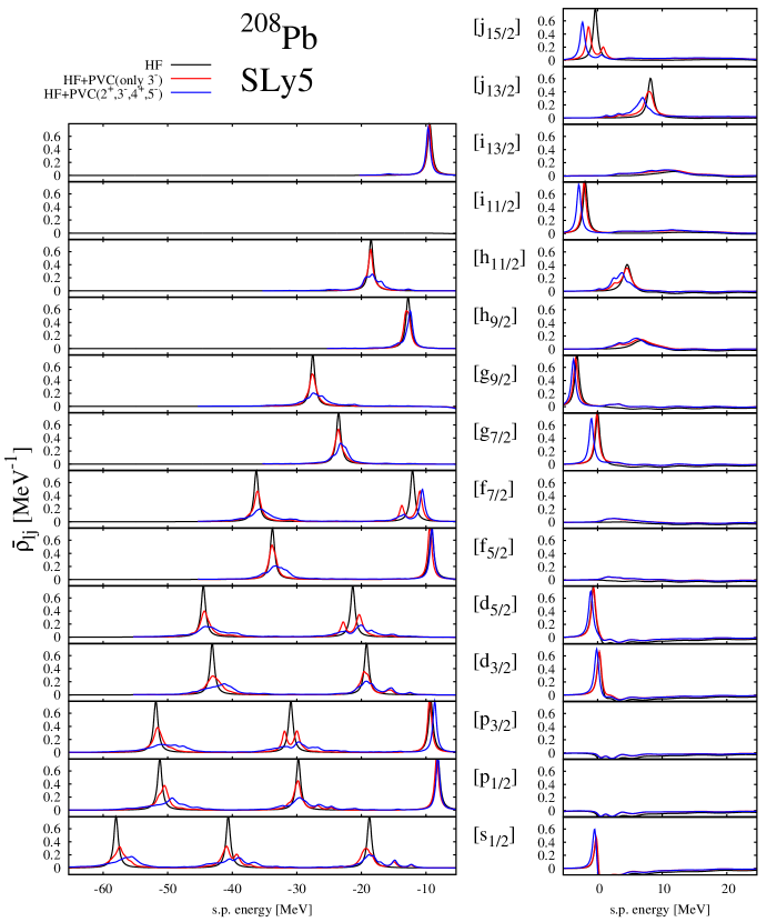
Figure 15: (Color online) The same as Fig. 7 in the case of ²⁰⁸Pb.

In many cases, the strong broadening of the single-particle strength observed in Fig. 15 is caused mostly by the coupling with the ISGQR and ISGOR, due to the favourable matching with the difference between the relevant single-particle states. This is the case for the orbitals $(1\rm s_{1/2})^{-1}$ and $(2\rm s_{1/2})^{-1}$, which couple to $\rm d_{3/2},\ \rm d_{5/2}\otimes 2^{+}$ and to $\rm f_{5/2},\ \rm f_{7/2}\otimes 3^{-}$. The contribution of the $4^{+}$ strength is small, but not completely negligible. The main configurations contributing to the large broadening of the $(3\rm s_{1/2})^{-1}$are $\rm f_{5/2},\ \rm f_{7/2}\otimes 3^{-}$. In the case of $(1\rm p_{1/2})^{-1}$ and $(2\rm p_{1/2})^{-1}$, the $2^{+}$, $3^{-}$ and $4^{+}$ phonons give comparable contributions to the strength fragmentation, which is also quite large. In the case of $(3\rm p_{1/2})$ and $(3\rm p_{3/2})^{-1}$, there is no good match with the energy of available single-particle configurations, and this explains the small amount of fragmentation that characterizes these states.

In the case of $(1\rm d_{3/2})^{-1}$, the $2^{+}$, $3^{-}$ and $4^{+}$ phonons give comparable contributions to the fragmentation. In the case of $(2\rm d_{3/2})^{-1}$, instead, the $3^{-}$ phonons play the most important role for the fragmentation: in fact, the relevant single-particle configurations are $(3\rm p_{3/2})^{-1}$, $(2\rm f_{5/2})^{-1}$, $(2\rm f_{7/2})^{-1}$ and $(1\rm h_{9/2})^{-1}$ coupled with the low-lying $3^{-}_{1}$ state. A similar pattern holds for the spin-orbit partners, that is, in the case of $(1\rm d_{5/2})^{-1}$, the $2^{+}$, $3^{-}$ and $4^{+}$ phonons give comparable contributions for the fragmentation but in the case of $(2\rm d_{5/2})^{-1}$, the $3^{-}$ phonons play the main role for the fragmentation (with some contribution arising from coupling with $4^{+}$ phonons). For $(2\rm d_{3/2})^{-1}$, the single-particle configurations involved are $(3\rm p_{3/2})^{-1}$, $(2\rm f_{5/2})^{-1}$, $(2\rm f_{7/2})^{-1}$ and $(1\rm h_{9/2})^{-1}$ (coupled with the $3^{-}_{1}$ state), as well as $(1\rm i_{13/2})^{-1}$. In the case of $(1\rm f_{5/2})^{-1}$ and $(1\rm f_{7/2})^{-1}$, the $2^{+}$, $3^{-}$ and $4^{+}$ phonons give similar contributions to the strength fragmentation; however, the main configuration involved turns out to be $(1\rm i_{13/2})^{-1}\otimes 3^{-}$. As already mentioned, the state $(2\rm f_{5/2})^{-1}$ is not affected much by the particle-vibration coupling. In the case of the states $(1\rm g_{7/2})$ and $(1\rm h_{9/2})^{-1}$, the $3^{-}$ is the main responsible for the couplings; however, the fragmentation is rather small, and the energy shift is also small. In the case of $(1\rm g_{9/2})^{-1}$, the $2^{+}$, $3^{-}$ and $4^{+}$ phonons give comparable effects. In the case of $(1\rm h_{11/2})^{-1}$, the fragmentation is caused by the coupling with the configurations $(3\rm p_{3/2})^{-1}$, $(2\rm f_{5/2})^{-1}$, $(2\rm f_{7/2})^{-1}$ and $(1\rm h_{9/2})^{-1}$ $\otimes$ 4⁺. The state $2\rm h_{11/2}$ is a resonant state in the continuum: $2^{+}$ and $3^{-}$ give the main contributions to fragment its strength: $1\rm j_{15/2}\otimes 2^{+}$, $3\rm d_{5/2},\ 2\rm g_{7/2},\ 2\rm g_{9/2},\ 1\rm i_{11/2}\otimes 3^{-}$ are the main states that produce the strength fragmentation. Also $1\rm j_{13/2}$ is a resonant state in the continuum: in this case, $3^{-}$ and $5^{-}$ are the most relevant phonons for the fragmentation of the strength: the main configurations are $2\rm g_{7/2}$, $2\rm g_{9/2}$, $1\rm i_{11/2}\otimes 3^{-}$ and $3\rm d_{3/2}$, $3\rm d_{5/2}$, $2\rm g_{7/2}$, $2\rm g_{9/2}$, $1\rm i_{11/2}\otimes 5^{-}$. Finally, in the case of the state $1\rm j_{15/2}$, the fragmentation is mainly caused by the coupling with the configurations $1\rm i_{11/2},2\rm g_{9/2}\otimes 3^{-}$. Once more, from considerations related to the matching of initial and intermediate energies, we expect that the low-lying $3^{-}$ state is the main contributor.

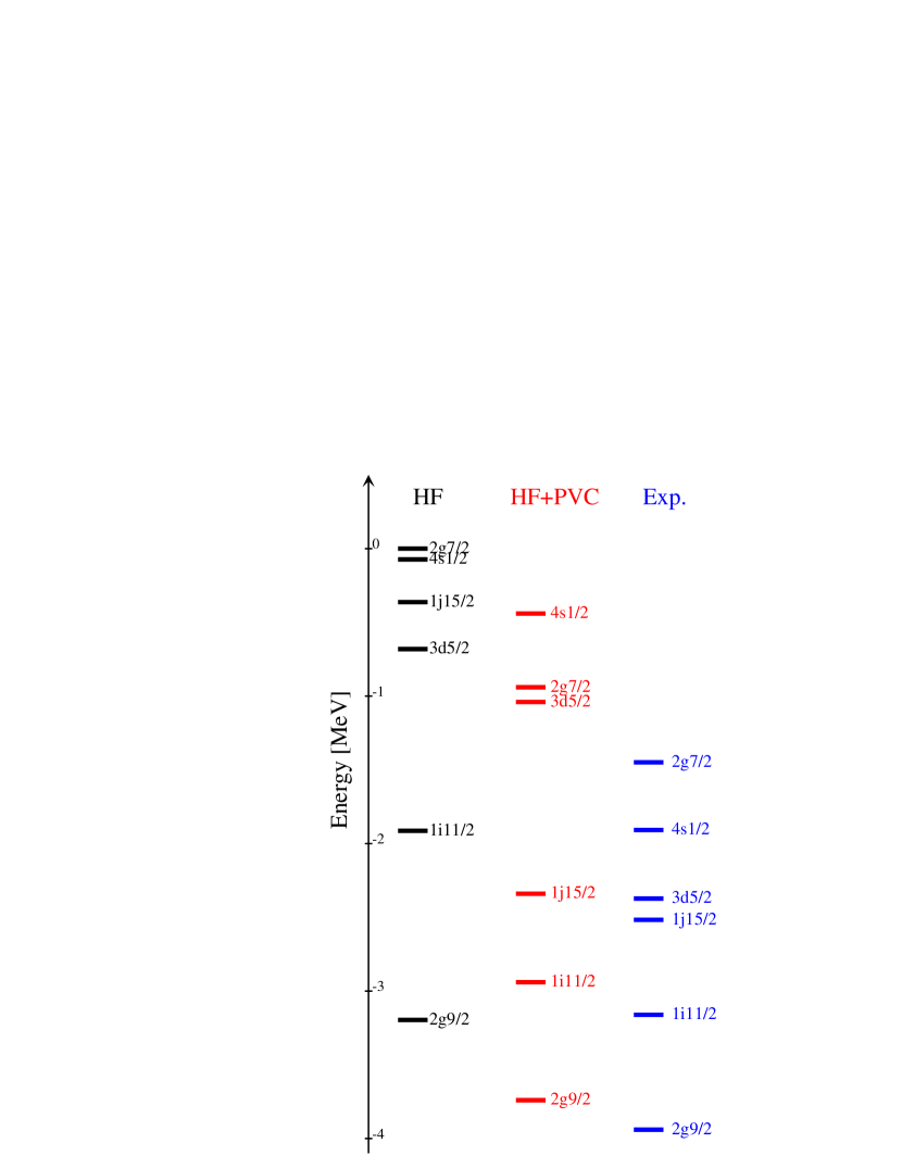
Figure 16: (Color online) Neutron particle states in ²⁰⁸Pb.

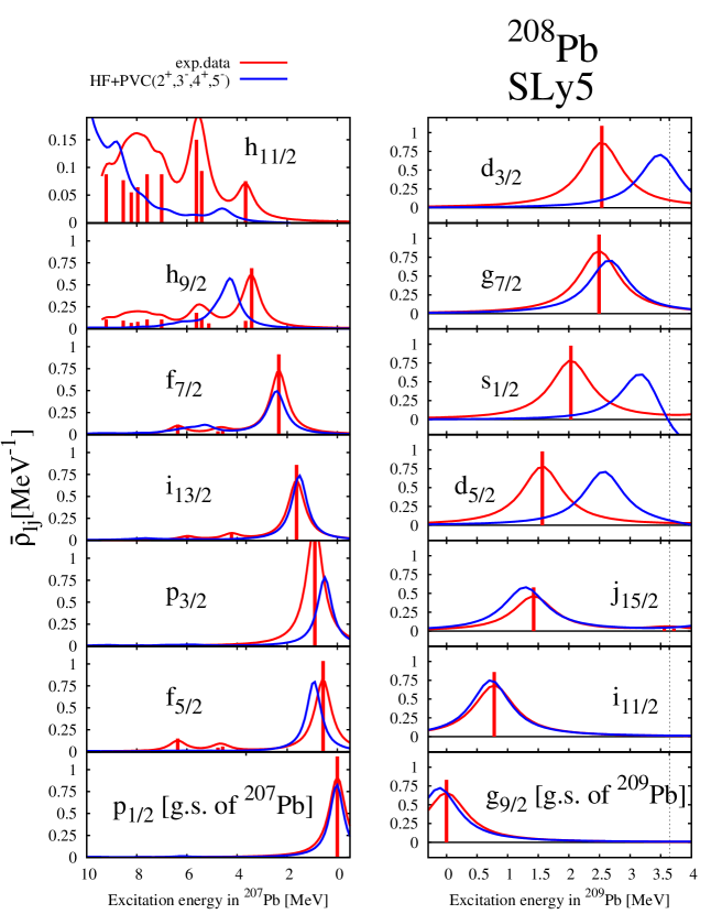
Figure 18: (Color online) The same as Fig. 12 in the case of ²⁰⁸Pb. The experimental data are taken from nucldataA207 ; nucldataA209 .

208Pb
Holes				Particles
	$S_{lj}(^{207}$Pb)				$S_{lj}(^{209}$Pb)
$J^{\pi}$	Exp.	Theory		$J^{\pi}$	Exp.	Theory
p1/2	1.07	0.82		g9/2	0.76	0.77
p3/2	1.50	0.84		s1/2	0.87	0.47
f5/2	1.07	0.84		d3/2	0.93	0.52
f7/2	1.02	0.84		d5/2	0.85	0.75
h9/2	1.53	0.86		g7/2	0.90	0.74
h11/2	0.69	0.39		i11/2	0.70	0.82
i13/2	0.90	0.87		j15/2	0.54	0.71

Table 6: The same as Table 3 for ²⁰⁸Pb.

The cumulative level densities of the various orbitals are compared in Fig. 18 to spectroscopic factors obtained from the ${}^{208}\mbox{\rm Pb}(^{3}\mbox{\rm He},\alpha)$ stripping reaction for hole states, and from ${}^{208}\mbox{\rm Pb}(\rm d,\rm p)$ reaction nucldataA207 ; nucldataA209 for particle states. The integrated level density is compared to the sum of experimental spectroscopic factors in Table 6. The quasiparticle character of the orbitals lying close to the Fermi energy is a general result of our adopted theoretical framework. Our results are in fair overall agreement with the experimental findings from transfer reactions, which were able to locate most of the quasiparticle strength associated with the orbitals lying close to the Fermi energy. The quality of the agreement varies from one case to the other, and it is hard to decide whether this has to be attributed either to specific features of our model, or to deficiencies in the experimental extraction of the spectroscopic factors (as testified, e.g., by the fact that some of them exceed the maximum allowed value of one). Furthermore, we must recall that (e,e^′p) experiments lead to much smaller spectroscopic factors, and that the relationship between the two kinds of experiments, as well as the reletive role of long- and short-range correlations, is a matter which continues to be actively debated kramer ; dickhoff . Last but not least, the very possibility of extracting a spectroscopic factor as a true observable, has been recently questioned hammer ; jennings .

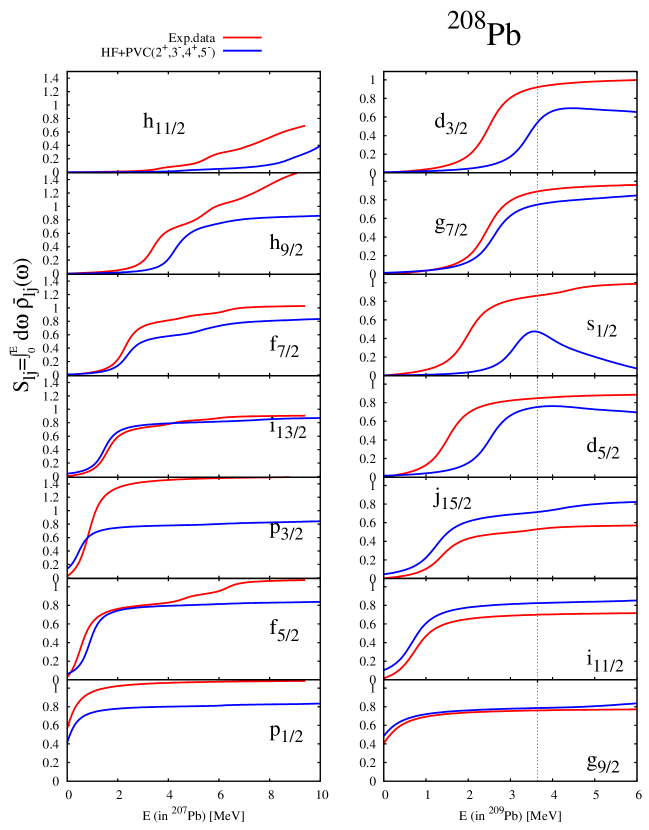
Figure 19: (Color online) The same as Fig. 13 in the case of ²⁰⁸Pb.

III.3 Results for ²⁴O

In this subsection, we finally give results for ²⁴O, as an example of neutron-rich, weakly bound ($S_{n}=$ 4.1 MeV) nucleus. This nucleus is a doubly magic isotope, due to to the usual proton shell closure at Z=8 and to an “exotic” neutron shell gap appearing at N=16. The magicity of ²⁴O, had been suggested by theoretical studies magic24a ; magic24b ; magic24c , and has been established by the measurement of the (unbound) ²⁵O ground-state and of its decay spectrum to ²⁴O, and by the extraction of the N=16 single-particle gap from the ^23,24,25O ground-state energies Hof08 ; Hof09 . As already mentioned, having a tool that allows studying weakly-bound systems by taking proper care of the continuum, is one of the main motivations of the present work. Interestingly enough, it has been suggested that nuclei in which the neutron separation energy becomes smaller than the proton separation energy are characterized by larger single-particle spectroscopic factors or, in other words, by more pure single-particle states. This is the feature emerging by the plot shown in Fig. 6 of Ref. Gade and consequently, one of those that can be analyzed within our framework. We will come back to this point below.

In Table 7 we provide the HF single-particle spectrum for neutrons. In Fig. 20, we illustrate our results for the RPA strength functions. Experimental information, although scarce, is available. The main results are that (i) there should be no bound excited state Stan04 , and (ii) the lowest excitation should be a 2⁺ state lying at 4.72 MeV Hof09 . In our RPA spectra, the lowest peak among those found for the chosen multipolarities is indeed a 2⁺ one, and its energy and electromagnetic transition probability are 3.4 MeV and 4.2 e² fm⁴. Experiment has also provided indications for the existence of a $1^{+}$ state lying at 5.33 MeV, but our calculations are limited to natural-parity states. In the case of this nucleus we compute the 1^- strength as well. To ensure that coupling with 1^- phonons does not introduce any error associated with spurious strength associated with the translational mode, we follow the procedure already discussed in our previous paper spurious . We find a significant amount of dipole strength lying at energies somewhat below the usual (IS and IV) giant dipole resonances.

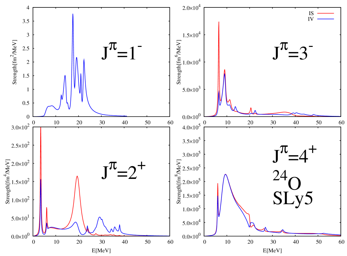
Figure 20: (Color online) The RPA strength functions in ²⁴O obtained with the present continuum RPA.

Nucleus	hole states[MeV]		particle states[MeV]
24O	1s$\frac{1}{2}$	-39.2	1d$\frac{3}{2}$	-1.3
	2s$\frac{1}{2}$	-5.3
	1p$\frac{1}{2}$	-17.2
	1p$\frac{3}{2}$	-22.0
	1d$\frac{5}{2}$	-7.5

Table 7: Skyrme Hartree-Fock single-particle energies for ²⁴O with the interaction SLy5. Hole and particle states at negative energies are displayed.

In Fig. 21, we display our results for the level density of ²⁴O. Before entering into some detail, we discuss the main emerging features and compare with what is known experimentally. In our calculation, the 1d_3/2 and 2s_1/2 states have a marked quasiparticle character, namely they are associated with a single narrow peak. It makes sense, therefore, to compare the experimental value of the gap with the HF and HF-PVC results for the energy difference between the 1d_3/2 and 2s_1/2 states, that is, 4.0 and 4.6 MeV respectively. The HF-PVC result is in good agreement with the experimental value of 4.86 MeV. In heavy nuclei, as a rule, the PVC shrinks the single-particle gap and increases the effective mass (cf. the previous subsection), but this is not the case in light nuclei due to the specific effect of having only low angular momentum occupied states (as already noticed in Ref. colo10 ). In the present case, while the PVC pushes the 1d_3/2 orbital closer to the Fermi energy (-2.5 MeV compared to the HF value of -1.3 MeV), the 2s_1/2 hole state is pushed further from it (-7.1 MeV compared to the HF value of -5.3 MeV).

The peak energies of the other orbitals obtained by using HF-PVC (HF) read 2.4 MeV (4.3 MeV) for 1f_7/2, and -8.3 MeV (-7.5 MeV) for 1d_5/2. The net effect of PVC is a shift down of the states. The absolute value of the energies is expected to depend on the choice of the effective force. Skyrme forces, as other mean-field frameworks, tend to predict larger binding in light neutron-rich nuclei as compared with the experimental findings, as it is clearly testified by the fact that ²⁸O turns out to be bound in many of these models. In the present case, the 1d_3/2 state is bound while it should be a resonant state. We can nonetheless look at relative energy differences. The known states in ²³O taken from Ref. Shi07 are, in addition to the 1/2⁺ ground-state, a 5/2⁺ state at 2.79 MeV and a 3/2⁺ at 4.04 MeV (leaving aside the state at 5.34 whose character is not clear, being either 3/2^- or 7/2^-). These are states that can decay to the ²²O ground state. In our calculation we can identify states below the energy threshold for this kind of decay: in particular the first 5/2⁺ state lies at 1.2 MeV in our calculation.

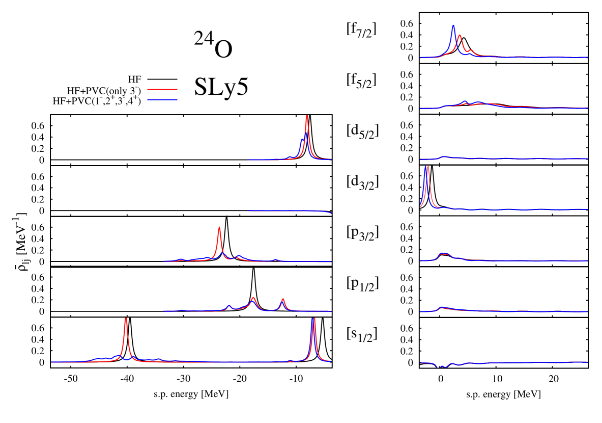
Figure 21: (Color online) The same as Fig. 7 in the case of ²⁴O. In this case not only 2⁺, 3^- and 4⁺ phonons but 1^- phonons as well are considered in the case of the full PVC result (blue curve).

We now discuss, the couplings that produce fragmentation of most of the single-particle strength distributions. At variance with the state 2s_1/2, the state 1s_1/2 is strongly fragmented. This fragmentation is chiefly caused by the configurations 1d${}_{5/2}^{-1}\otimes\ 2^{+}$ and $(1\rm p_{1/2})^{-1},\ (1\rm p_{3/2})^{-1}\otimes 1^{-}$. By inspecting the energy difference, we can assume that the IVGQR and IVGDR play the main role for the fragmentation. The state $(1\rm p_{1/2})^{-1}$ is fragmented due to the coupling with the configuration $(1\rm d_{5/2})^{-1}\otimes 3^{-}$: we expect that the ISGOR and IVGOR play the main role by considering the energy matching. $(2\rm s_{1/2})^{-1}\otimes 1^{-}$ can also contribute to the fragmentation, yet to a minor extent. The main configuration giving rise to the fragmentation of the state $(1\rm p_{3/2})^{-1}$ is the configuration $(1\rm d_{5/2})^{-1}\otimes 1^{-}$. Here, due to the energy difference between the hole states $(1\rm p_{3/2})^{-1}$ and $(1\rm d_{5/2})^{-1}$, the dipole excitations around $14$ MeV do play the main role. In the case of the fragmentation of the $(1\rm d_{5/2})^{-1}$ state, the configuration $(2\rm s_{1/2})^{-1}\otimes 2^{+}$ is the most important one, and the low-lying $2^{+}$ state at 3.4 MeV is the most relevant. Finally, the energy shift of the state $1\rm f_{7/2}$ is mostly caused by the coupling with the configuration $1\rm d_{3/2}\otimes 3^{-}$.

24O
Holes				Particles
	$S_{lj}(^{24}$O)				$S_{lj}(^{24}$O)
$J^{\pi}$	Exp.	Theory		$J^{\pi}$	Exp.	Theory
s1/2	—	0.81		d3/2	—	0.83
d5/2	—	0.78

Table 8: The same as Table 3 for ²⁴O.

Last but not least, we come back to the point raised above, namely that the (quasi-particle-like) states around the Fermi energy, 1d_3/2 and 2s_1/2, are quite pure (see also Table 8). In our calculation, there are not optimal energy matching of those states with other configurations due to the scarcity of low-lying collective excitations and large gaps between single-particle state. More generally, in our calculations the coupling of neutron states is mainly with the proton component of the phonon states (due to the dominance of the neutron-proton interaction). Therefore, neutron states on neutron-rich nuclei are expected to be more pure because proton excitations are pushed at higher energy as the neutron excess increases. Recently, other calculations of the spectroscopic factors in light nuclei within the coupled-cluster approach have become available in Ref. jensen (see also the critical discussion in Ref. hagen ).

IV Summary

The idea that single-particle strength is not systematically pure in atomic nuclei, and that coupling with other degrees of freedom is quite relevant, is an old idea in nuclear physics. Phenomenological calculations based on particle-vibration coupling (PVC) for spherical nuclei have been performed for several deacades, and they have been quite instrumental to point out some of the limitations of the pure mean-field approach (like, e.g., the enhancement of the effective mass around the Fermi energy). Microscopic PVC calculations based on the consistent use of an effective Hamiltonian, have become available only recently.

None of the mentioned calculations, to our knowledge, takes proper care of the continuum. In our work, for the first time, we have implemented a scheme based on coordinate-space representation in which the single-particle states, the vibrations, and their coupling are calculated with proper inclusion of the continuum. This is of special interest if weakly-bound nuclei close to the drip lines are to be studied. However, also in well-bound nuclei the present approach present advantages in the sense that resonant states can be properly studied. Transfer to the continuum has been the subject of several experimental studies.

In stable nuclei we obtain results that are in overall agreement with previous studies. We can, at the same time, better describe the fragmentation of the single-particle strength. The shifts of the single-particle states around the Fermi energy, with respect to the HF values, are relatively large (in keeping also with the fact that we cannot restrict our coupling to collective states only). We obtain an overall agreement with experiment in ²⁰⁸Pb, while in the case of ⁴⁰Ca our results point to the need of re-fitting the Skyrme interaction that has been devised to work at the mean-field level and not beyond it.

We have also applied our model to a neutron-rich nucleus, namely ²⁴O. This is a double-magic nucleus, and there are few low-lying states. Because of this, and also since the neutron states energy would be more affected by coupling with protons, the neutron single-particle strength around the Fermi energy is quite pure (i.e., spectroscopic factors are rather close to one). While this is in agreement with some experimental findings, certainly more detailed spectroscopic studies are needed to extract a global trend and a firm understanding.

Appendix A Hartree-Fock Green’s function

As it is stated in the main text, it is necessary to use the causal Green’s function for the Dyson equation because this equation is based on the use of the Wick’s theorem, and the Wick’s theorem applies only to time-ordered products. On the other hand, the continuum HF Green’s function is given in the form of a retarded function. So we need to compute the causal Green’s function starting from the retarded Green’s function in order to use the continuum HF Green’s function in the Dyson equation.

The causal HF Green’s function is defined by

$$iG_{0}^{C}(\mbox{\boldmath$r$}\sigma t,\mbox{\boldmath$r$}^{\prime}\sigma^{\prime}t^{\prime}) \equiv \langle\Psi_{0}|\mbox{T}\{\hat{\psi}(\mbox{\boldmath$r$}\sigma t)\hat{\psi}^{\dagger}(\mbox{\boldmath$r$}^{\prime}\sigma^{\prime}t^{\prime})\}|\Psi_{0}\rangle$$

$$= \theta(t-t^{\prime})\langle\Psi_{0}|\hat{\psi}(\mbox{\boldmath$r$}\sigma t)\hat{\psi}^{\dagger}(\mbox{\boldmath$r$}^{\prime}\sigma^{\prime}t^{\prime})|\Psi_{0}\rangle-\theta(t^{\prime}-t)\langle\Psi_{0}|\hat{\psi}^{\dagger}(\mbox{\boldmath$r$}^{\prime}\sigma^{\prime}t^{\prime})\hat{\psi}(\mbox{\boldmath$r$}\sigma t)|\Psi_{0}\rangle.$$

The retarded Green’s function is instead defined by

$$iG^{R}_{0}(\mbox{\boldmath$r$}\sigma t,\mbox{\boldmath$r$}^{\prime}\sigma^{\prime}t^{\prime}) \equiv \theta(t-t^{\prime})\langle\Psi_{0}|\{\hat{\psi}(\mbox{\boldmath$r$}\sigma t),\hat{\psi}^{\dagger}(\mbox{\boldmath$r$}^{\prime}\sigma^{\prime}t^{\prime})\}|\Psi_{0}\rangle.$$ (28)

From these two definitions, and using $\theta(t^{\prime}-t)=1-\theta(t-t^{\prime})$, we can find that

$$iG^{C}_{0}(\mbox{\boldmath$r$}\sigma t,\mbox{\boldmath$r$}^{\prime}\sigma^{\prime}t^{\prime})=iG^{R}_{0}(\mbox{\boldmath$r$}\sigma t,\mbox{\boldmath$r$}^{\prime}\sigma^{\prime}t^{\prime})-\sum_{h}e^{-\frac{i}{\hbar}e_{h}(t-t^{\prime})}\phi_{h}^{*}(\mbox{\boldmath$r$}^{\prime}\sigma^{\prime})\phi_{h}(\mbox{\boldmath$r$}\sigma)$$ (29)

The Fourier transform of Eq. (29) is expressed as

$$G^{C}_{0}(\mbox{\boldmath$r$}\sigma,\mbox{\boldmath$r$}^{\prime}\sigma^{\prime};\omega) = G^{R}_{0}(\mbox{\boldmath$r$}\sigma,\mbox{\boldmath$r$}^{\prime}\sigma^{\prime};\omega)+\sum_{h}\frac{2i\eta}{(\omega-e_{h})^{2}+\eta^{2}}\phi_{h}(\mbox{\boldmath$r$}\sigma)\phi_{h}^{*}(\mbox{\boldmath$r$}^{\prime}\sigma^{\prime})$$ (31)

(in the limit $$\eta\to 0$$)

$$\to G^{R}_{0}(\mbox{\boldmath$r$}\sigma,\mbox{\boldmath$r$}^{\prime}\sigma^{\prime};\omega)+2\pi i\sum_{h}\delta(\omega-e_{h})\phi_{h}(\mbox{\boldmath$r$}\sigma)\phi_{h}^{*}(\mbox{\boldmath$r$}^{\prime}\sigma^{\prime})$$ (32)

The continuum HF Green’s function $G_{0,lj}$ given by Eq. (15) is regular for the complex energy $E$. So the retarded Green’s function with a smearing width $\eta$ is expressed as

$$G^{R}_{0,lj}(rr^{\prime},\omega)=G_{0,lj}(rr^{\prime};\omega+i\eta),$$ (33)

where $\omega$ is the real part of the complex energy. Then the continuum causal Green’s function can be expressed by

$$G^{C}_{0,lj}(rr^{\prime},\omega)=G_{0,lj}(rr^{\prime};\omega+i\eta)+\sum_{n_{h}l_{h}j_{h}}\frac{2i\eta}{(\omega-e_{n_{h}l_{h}j_{h}})^{2}+\eta^{2}}\phi_{n_{h}l_{h}j_{h}}(r)\phi_{n_{h}l_{h}j_{h}}(r^{\prime}).$$ (34)

Appendix B Unperturbed response function

In general, the RPA theory can be formulated in two ways. One is based on the causal function, while another one on the retarded function. Both formulations give the same results for the physical part of the spectrum, namely for positive excitation energy. However, a complete RPA basis must include negative energy states and the two aforementioned formulations are different for negative energies.

In order to construct the self-energy function of Eq. (7), we need to consider the RPA response function not only in the positive energy domain but also in the negative energy domain due to the required energy integration. So we cannot use the retarded RPA response function for the self-energy function. The RPA equation for the response function is given by $R=R_{0}+R_{0}\kappa R$ in any of the representations, $R_{0}$ being the unperturbed response function, and $R$ the RPA response function. In order to obtain the causal RPA response function by solving this equation, the causal unperturbed response function should be used.

Normally the continuum (Q)RPA is formulated by using retarded functions within the linear response theory. The continuum HF(B) Green’s function is used to build the (retarded) unperturbed response function sagawa ; matsuo1 . It is therefore necessary to know how to convert the retarded unperturbed response function to the causal function in the continuum RPA formalism. We show it in the present Appendix.

The causal and retarded response function in RPA are defined by

$$iR_{0}^{C}(\mbox{\boldmath$r$}t,\mbox{\boldmath$r$}^{\prime}t^{\prime}) = \langle\Psi_{0}|\mbox{T}\{\delta\hat{\rho}(\mbox{\boldmath$r$}t)\delta\hat{\rho}(\mbox{\boldmath$r$}^{\prime}t^{\prime})\}|\Psi_{0}\rangle$$ (35)

$$= \theta(t-t^{\prime})\langle\Psi_{0}|\delta\hat{\rho}(\mbox{\boldmath$r$}t)\delta\hat{\rho}(\mbox{\boldmath$r$}^{\prime}t^{\prime})|\Psi_{0}\rangle+\theta(t^{\prime}-t)\langle\Psi_{0}|\delta\hat{\rho}(\mbox{\boldmath$r$}^{\prime}t^{\prime})\delta\hat{\rho}(\mbox{\boldmath$r$}t)|\Psi_{0}\rangle$$ (36)

$$iR_{0}^{R}(\mbox{\boldmath$r$}t,\mbox{\boldmath$r$}^{\prime}t^{\prime}) = \theta(t-t^{\prime})\langle\Psi_{0}|[\delta\hat{\rho}(\mbox{\boldmath$r$}t),\delta\hat{\rho}(\mbox{\boldmath$r$}^{\prime}t^{\prime})]|\Psi_{0}\rangle,$$ (37)

respectively (here $|\Psi_{0}\rangle$ is the HF ground state). From these definitions, one can find the relation between them as follows,

$$iR_{0}^{C}(\mbox{\boldmath$r$}t,\mbox{\boldmath$r$}^{\prime}t^{\prime}) = iR_{0}^{R}(\mbox{\boldmath$r$}t,\mbox{\boldmath$r$}^{\prime}t^{\prime})+\langle\Psi_{0}|\delta\hat{\rho}(\mbox{\boldmath$r$}t)\delta\hat{\rho}(\mbox{\boldmath$r$}^{\prime}t^{\prime})|\Psi_{0}\rangle$$ (38)

$$= iR_{0}^{R}(\mbox{\boldmath$r$}t,\mbox{\boldmath$r$}^{\prime}t^{\prime})-\sum_{hh^{\prime}}e^{i(e_{h}-e_{h^{\prime}})(t-t^{\prime})}\phi_{h}^{*}(\mbox{\boldmath$r$})\phi_{h^{\prime}}(\mbox{\boldmath$r$})\phi_{h^{\prime}}^{*}(\mbox{\boldmath$r$}^{\prime})\phi_{h}(\mbox{\boldmath$r$}^{\prime}).$$ (39)

The Fourier transformation of the latter equation gives

$$R_{0}^{C}(\mbox{\boldmath$r$}\mbox{\boldmath$r$}^{\prime};\omega) = R_{0}^{R}(\mbox{\boldmath$r$}\mbox{\boldmath$r$}^{\prime};\omega)-\sum_{hh^{\prime}}\frac{2i\eta}{(\omega-e_{h^{\prime}}+e_{h})^{2}+\eta^{2}}\phi_{h}^{*}(\mbox{\boldmath$r$})\phi_{h^{\prime}}(\mbox{\boldmath$r$})\phi_{h^{\prime}}^{*}(\mbox{\boldmath$r$}^{\prime})\phi_{h}(\mbox{\boldmath$r$}^{\prime})w$$ (41)

$$(\mbox{in the limit of }\eta\to 0)$$

$$\to R_{0}^{R}(\mbox{\boldmath$r$}\mbox{\boldmath$r$}^{\prime};\omega)-2\pi i\sum_{hh^{\prime}}\delta(\omega-e_{h^{\prime}}+e_{h})\phi_{h}^{*}(\mbox{\boldmath$r$})\phi_{h^{\prime}}(\mbox{\boldmath$r$})\phi_{h^{\prime}}^{*}(\mbox{\boldmath$r$}^{\prime})\phi_{h}(\mbox{\boldmath$r$}^{\prime}),$$ (42)

where $R_{0}^{R}(\mbox{\boldmath$r$}\mbox{\boldmath$r$}^{\prime};\omega)$ can be expressed by means of the retarded HF Green’s function as

$$R_{0}^{R}(\mbox{\boldmath$r$}\mbox{\boldmath$r$}^{\prime};\omega) = \sum_{h}\phi_{h}^{*}(\mbox{\boldmath$r$})G_{0}^{R}(\mbox{\boldmath$r$}\mbox{\boldmath$r$}^{\prime};\omega+e_{h})\phi_{h}(\mbox{\boldmath$r$}^{\prime})+\phi_{h}^{*}(\mbox{\boldmath$r$}^{\prime})G_{0}^{R*}(\mbox{\boldmath$r$}\mbox{\boldmath$r$}^{\prime};-\omega+e_{h})\phi_{h}(\mbox{\boldmath$r$}).$$ (43)

In the continuum RPA formalism, the continuum HF Green’s function is used as $G^{R}_{0}$ in Eq. (43).

Appendix C Spectral representation of the Green’s function and the response function

Here we show the spectral representations of the HF Green’s function and the RPA response function (both causal and retarded). The difference will appear in the sign of the imaginary part $\eta$. Actually this is very important to obtain the proper self-energy function by using the contour integration, because this sign differencee produce changes in the position of the poles of the Green’s function and of the response function on the complex energy plane (this fact is connected with the fact that the Wick’s theorem can be applied only for the causal function, as already mentioned).

$$G^{C}_{0}(\mbox{\boldmath$r$}\sigma,\mbox{\boldmath$r$}^{\prime}\sigma^{\prime};\omega) =\sum_{h}\frac{\phi_{h}(\mbox{\boldmath$r$}\sigma)\phi^{*}_{h}(\mbox{\boldmath$r$}^{\prime}\sigma^{\prime})}{\omega-e_{h}-i\eta}+\sum_{p}\frac{\phi_{p}(\mbox{\boldmath$r$}\sigma)\phi^{*}_{p}(\mbox{\boldmath$r$}^{\prime}\sigma^{\prime})}{\omega-e_{p}+i\eta}$$ (44)

$$G^{R}_{0}(\mbox{\boldmath$r$}\sigma,\mbox{\boldmath$r$}^{\prime}\sigma^{\prime};\omega) =\sum_{h}\frac{\phi_{h}(\mbox{\boldmath$r$}\sigma)\phi^{*}_{h}(\mbox{\boldmath$r$}^{\prime}\sigma^{\prime})}{\omega-e_{h}+i\eta}+\sum_{p}\frac{\phi_{p}(\mbox{\boldmath$r$}\sigma)\phi^{*}_{p}(\mbox{\boldmath$r$}^{\prime}\sigma^{\prime})}{\omega-e_{p}+i\eta}$$ (45)

$$R_{C}(\mbox{\boldmath$r$}\mbox{\boldmath$r$}^{\prime};\omega) =\sum_{\nu}\frac{\langle 0|\hat{\rho}(\mbox{\boldmath$r$})|\nu\rangle\langle\nu|\hat{\rho}(\mbox{\boldmath$r$}^{\prime})|0\rangle}{\omega-E_{\nu}+i\eta}-\frac{\langle 0|\hat{\rho}(\mbox{\boldmath$r$}^{\prime})|\nu\rangle\langle\nu|\hat{\rho}(\mbox{\boldmath$r$})|0\rangle}{\omega+E_{\nu}-i\eta}$$

$$R_{R}(\mbox{\boldmath$r$}\mbox{\boldmath$r$}^{\prime};\omega) =\sum_{\nu}\frac{\langle 0|\hat{\rho}(\mbox{\boldmath$r$})|\nu\rangle\langle\nu|\hat{\rho}(\mbox{\boldmath$r$}^{\prime})|0\rangle}{\omega-E_{\nu}+i\eta}-\frac{\langle 0|\hat{\rho}(\mbox{\boldmath$r$}^{\prime})|\nu\rangle\langle\nu|\hat{\rho}(\mbox{\boldmath$r$})|0\rangle}{\omega+E_{\nu}+i\eta}$$ (47)

Appendix D Spectral representation of the self-energy function

The self-energy function in the space-time representation is defined by Eq. (4). If we insert the HF and the RPA results in this definition, then the self-energy function can be expressed as

$$\Sigma(\mbox{\boldmath$r$}_{1}\sigma_{1}t_{1},\mbox{\boldmath$r$}_{2}\sigma_{2}t_{2}) = \kappa(\mbox{\boldmath$r$}_{1})G_{0}(\mbox{\boldmath$r$}_{1}\sigma_{1}t_{1},\mbox{\boldmath$r$}_{2}\sigma_{2}t_{2})\kappa(\mbox{\boldmath$r$}_{2})iR(\mbox{\boldmath$r$}_{1}t_{1}\mbox{\boldmath$r$}_{2}t_{2})$$ (49)

$$= \frac{1}{i}\theta(t_{1}-t_{2})\sum_{p,\nu}e^{-i(E_{\nu}+e_{p})(t_{1}-t_{2})}\kappa(\mbox{\boldmath$r$}_{1})\delta\rho_{\nu}(\mbox{\boldmath$r$}_{1})\phi_{p}(\mbox{\boldmath$r$}_{1}\sigma_{1})\phi_{p}^{*}(\mbox{\boldmath$r$}_{2}\sigma_{2})\delta\rho_{\nu}^{*}(\mbox{\boldmath$r$}_{2})\kappa(\mbox{\boldmath$r$}_{2})$$

$$-\frac{1}{i}\theta(t_{2}-t_{1})\sum_{h,\nu}e^{+i(E_{\nu}-e_{h})(t_{1}-t_{2})}\kappa(\mbox{\boldmath$r$}_{1})\delta\rho_{\nu}^{*}(\mbox{\boldmath$r$}_{1})\phi_{h}^{*}(\mbox{\boldmath$r$}_{1}\sigma_{1})\phi_{h}(\mbox{\boldmath$r$}_{2}\sigma_{2})\delta\rho_{\nu}(\mbox{\boldmath$r$}_{2})\kappa(\mbox{\boldmath$r$}_{2})$$

The Fouriter transform of Eq. (49) gives

$$\Sigma(\mbox{\boldmath$r$}\sigma,\mbox{\boldmath$r$}^{\prime}\sigma^{\prime};\omega) = \sum_{h,\nu}\frac{\phi_{h}(\mbox{\boldmath$r$}\sigma)\delta\rho^{*}_{\nu}(\mbox{\boldmath$r$})\kappa(\mbox{\boldmath$r$})\phi_{h}^{*}(\mbox{\boldmath$r$}^{\prime}\sigma^{\prime})\delta\rho_{\nu}(\mbox{\boldmath$r$}^{\prime})\kappa(\mbox{\boldmath$r$}^{\prime})}{\omega-e_{h}+E_{\nu}-i\eta}$$ (50)

$$\hskip 28.45274pt+\sum_{p,\nu}\frac{\phi_{p}(\mbox{\boldmath$r$}\sigma)\delta\rho_{\nu}(\mbox{\boldmath$r$})\kappa(\mbox{\boldmath$r$})\phi_{p}^{*}(\mbox{\boldmath$r$}^{\prime}\sigma^{\prime})\delta\rho^{*}_{\nu}(\mbox{\boldmath$r$}^{\prime})\kappa(\mbox{\boldmath$r$}^{\prime})}{\omega-e_{p}-E_{\nu}+i\eta}$$

Appendix E Residual interaction within the Landau-Migdal approximation

Here we show the explicit expression of the residual interaction within the so-called Landau-Migdal approximation. This residual force is used in the self-energy function [Eq. (13)].

$$\kappa_{qq^{\prime}}(r) = \frac{\partial h_{q}}{\partial\rho_{q^{\prime}}}(r)=\frac{\delta^{2}E}{\delta\rho_{q}\delta\rho_{q^{\prime}}}\hskip 28.45274pt\mbox{where $q,p$}$$ (58)

$$= \left\{\begin{array}[]{cl}(q=q^{\prime})&\displaystyle{\frac{t_{0}}{2}(1-x_{0})}\\ &\displaystyle{+\frac{t_{3}}{12}\rho^{\gamma}\Big{[}(\gamma+2)(\gamma+1)(1+\frac{x_{3}}{2})-(x_{3}+\frac{1}{2})\left(2+4\gamma\frac{\rho_{q}}{\rho}+\gamma(\gamma-1)\sum_{\alpha}\left(\frac{\rho_{\alpha}}{\rho}\right)^{2}\right)\Big{]}}\\ &\displaystyle{+\frac{1}{4}\left(t_{1}(1-x_{1})+3t_{2}(1+x_{2})\right)k_{F}^{2}}\\ &\\ (q\neq q^{\prime})&\displaystyle{t_{0}(1+\frac{x_{0}}{2})}\\ &\displaystyle{+\frac{t_{3}}{12}\rho^{\gamma}\Big{[}(\gamma+2)(\gamma+1)(1+\frac{x_{3}}{2})-(x_{3}+\frac{1}{2})\left(2\gamma+\gamma(\gamma-1)\sum_{\alpha}\left(\frac{\rho_{\alpha}}{\rho}\right)^{2}\right)\Big{]}}\\ &\displaystyle{+\frac{1}{2}\left(t_{1}(1+\frac{x_{1}}{2})+t_{2}(1+\frac{x_{2}}{2})\right)k_{F}^{2}}\end{array}\right.$$

References

- (1) P. F. Bortignon, G. Colò, H. Sagawa, J. Phys. G 37, 064013 (2010).
- (2) M. Stoitsov, M. Kortelainen, S. K. Bogner, T. Duguet, R. J. Furnstahl, B. Gebremariam, and N. Schunck, Phys. Rev. C 82, 054307 (2010).
- (3) A. Bohr, B. R. Mottelson, Nuclear Structure. Vol. II (W.A. Benjamin, New York, 1971).
- (4) C. Mahaux, P. F. Bortignon, R. A. Broglia, C. H. Dasso, Phys. Rep. 120, 1 (1985).
- (5) F. Barranco, R. A. Broglia, G. Gori, E. Vigezzi, P. F. Bortignon, and J. Terasaki, Phys. Rev. Lett. 83, 2147 (1999).
- (6) A. V. Avdeenkov and S. P. Kamerdjev, JETP Lett. 69, 669 (1999).
- (7) A. Pastore, F. Barranco, R. A. Broglia, and E. Vigezzi, Phys. Rev. C78, 024315 (2008).
- (8) A. Idini, F. Barranco, R.A. Broglia and E. Vigezzi, Phys. Rev. C 85, 014331 (2012).
- (9) K. Hebeler, T. Duguet, T. Lesinski, and A. Schwenk, Phys. Rev. C 80, 044321 (2019).
- (10) M. Baldo, U. Lombardo, S. S. Pankratov, and E. E. Saperstein, J. Phys. G: Nucl. Part. Phys. 37, 064016 (2010).
- (11) V. Somà, T. Duguet and C. Barbieri, Phys. Rev C 84, 024312 (2012).
- (12) H. Hergert and R. Roth, Phys. Rev. C 80, 024312 (2009).
- (13) G. Colò, H. Sagawa, P. F. Bortignon, Phys. Rev. C82, 064307 (2010).
- (14) E. Litvinova, P. Ring, Phys. Rev. C73, 044328 (2006).
- (15) E. V. Litvinova and A. V. Afanasjev, Phys. Rev. C84, 014305 (2011).
- (16) G. Colò, P. F. Bortignon and R. A. Broglia, Nucl. Phys. A649, 335c (1999).
- (17) M. Matsuo, Nucl. Phys. A696, 371 (2001).
- (18) K. Mizuyama, M. Matsuo, and Y. Serizawa, Phys. Rev. C79, 024313 (2009).
- (19) G. F. Bertsch and S. F. Tsai, Phys. Rep. 18, 125 (1975).
- (20) S. Shlomo and G. F. Bertsch, Nucl. Phys. A 243, 507 (1975).
- (21) K. F. Liu and N. Van Giai, Phys. Lett. B 65, 23 (1976).
- (22) A. L. Fetter, J. D. Walecka, Quantum Theory of Many-Particle Systems (McGraw-Hill, New York, 1971).
- (23) R. D. Mattuck, A Guide to Feynman Diagrams in the Many-Body Problem (Dover Publications, New York, 1992).
- (24) H. Sagawa, Prog. Theor. Phys. Suppl. 142, 1 (2001).
- (25) S. Shlomo, Nucl. Phys. A539, 17 (1992).
- (26) E. Chabanat, P. Bonche, P. Haensel, J. Meyer and R. Schaeffer, Nucl. Phys. A643, 441 (1998).
- (27) K. Moghrabi, M. Grasso, G. Colò and N. Van Giai, Phys. Rev. Lett. 105, 262501 (2010); K. Moghrabi, M. Grasso, X. Roca-Maza, and G. Colò, Phys. Rev. C85, 044323 (2012).
- (28) T. Kibédi and R.H. Spear, Atomic Data and Nuclear Data Tables 80, 35 (2002).
- (29) J.A. Cameron and B. Singh, Nuclear Data Sheets 102, 293 (2004).
- (30) B. Singh and J.A. Cameron, Nuclear Data Sheets 107, 225 (2006).
- (31) J.A. Cameron and B. Singh, Nuclear Data Sheets 94, 429 (2001).
- (32) R. Satchler, Direct nuclear reactions (Oxford University Press, Oxford, 1983).
- (33) F.J. Eckle, H. Lenske, G. Eckle, G. Graw, R. Hertenberger, H. Kader, H.J. Maier, F. Merz, H. Nann, P. Schiemenz and H.H. Wolter, Nucl. Phys. A506, 159 (1990).
- (34) M.N. Harakeh, A. van der Woude, Giant resonances. Fundamental High-Frequency Modes of Nuclear Excitation (Oxford University Press, Oxford, 2001).
- (35) S. Kamerdzhiev, J. Speth and G. Tertychny, Phys. Rep. 393, 1 (2004).
- (36) S. Raman, C.W. Nestor and P. Tikkanen, Atomic Data and Nuclear Data Tables 78, 1 (2001).
- (37) F.G. Kondev and S. Lalkovski, Nuclear Data Sheets 112, 707 (2011).
- (38) M.J. Martin, Nuclear Data Sheets 63, 723 (1991).
- (39) G.J. Kramer, H.P. Block and L. Lapikás, Nucl. Phys. A679, 267 (2001).
- (40) W.H. Dickhoff and D. Van Neck, Many-Body Exposed ! (World Scientific, Singapore, 2005).
- (41) R.J. Furnstahl and H.W. Hammer, Phys. Lett. B531, 203 (2002).
- (42) B.K. Jennings (2011), arXiv:1102.3721.
- (43) B.A. Brown and W.A. Richter, Phys. Rev. C74, 034315 (2004)
- (44) Y. Utsuno, T. Otsuka, T. Misuzaki and M. Honma, Phys. Rev. C60, 054315 (1999)
- (45) T. Otsuka et al., Phys. Rev. Lett. 87, 082502 (2001).
- (46) C.R. Hoffman et al., Phys. Rev. Lett. 100, 152502 (2008).
- (47) C.R. Hoffman et al., Phys. Lett. B672, 17 (2009).
- (48) A. Gade et al., Phys. Rev. C77, 044306 (2008).
- (49) M. Stanoiou et al., Phys. Rev, C69, 034312 (2004).
- (50) K. Mizuyama and G. Colò, Phys. Rev. C85, 024307 (2012).
- (51) A. Schiller et al., Phys. Rev. Lett. 99, 112501 (2007).
- (52) Ø. Jensen, G. Hagen, M. Hjorth-Jensen, B.A. Brown, and A. Gade, Phys. Rev. Lett. 107, 032501 (2011).
- (53) T. Duguet and G. Hagen, Phys. Rev. C85, 034330 (2012).