Modeling the irregularities of solar cycle using flux transport dynamo models

Abstract

The sunspot number varies roughly periodically with time. However the individual cycle durations and the amplitudes are found to vary in an irregular manner. It is observed that the stronger cycles are having shorter rise times and vice versa. This leads to an important effect know as the Waldmeier effect. Another important feature of the solar cycle irregularity are the grand minima during which the activity level is strongly reduced. We explore whether these solar cycle irregularities can be studied with the help of the flux transport dynamo model of the solar cycle. We show that with a suitable stochastic fluctuations in a regular dynamo model, we are able to reproduce many irregular features of the solar cycle including the Waldmeier effect and the grand minimum. However, we get all these results only if the value of the turbulent diffusivity in the convection zone is reasonably high.

1 INTRODUCTION

Although the sunspot number varies periodically with time with an average period of 11 year, the individual cycle period (length) and also the strength (amplitude) vary in a random way. It is observed that the stronger cycles have shorter periods and vice versa. This leads to an important feature of solar cycle known as Waldmeier effect. It says that there is an anti-correlation between the rise time and the peak sunspot number. We call this as WE1. Now instead of rise time if we consider the rise rate then we get very tight positive correlation between the rise rate and the peak sunspot number. We call this as WE2.

Another important aspect of solar activity are the grand minima. These are the periods of strongly reduced activity. A best example of these is the Maunder minimum during during 1645–1715. It was not an artifact of few observations, but a real phenomenon (Hoyt & Schatten 1996). From the study of the cosmogenic isotope ¹⁴C data in tree rings, Usoskin et al. (2007) reported that there are $27$ grand minimum during last $11,000$ years.

2 METHODOLOGY AND RESULTS

We want to model these irregularities of solar cycle using flux transport dynamo model (Choudhuri et al. 1995; Dikpati & Charbonneau 1999; Chatterjee et al. 2004). In this model, the turbulent diffusivity is an important ingredient which is not properly constrained. Therefore several groups use different value of diffusivity and this leads to two kinds of flux transport dynamo model – high diffusivity model and low diffusivity model. In the earlier model, the value of diffusivity usually used is $\sim 10^{12}-10^{13}$ cm² s^-1 (see also Jiang et al. 2007 and Yeates et al. 2008 for details), whereas in the latter model, it is $\sim 10^{10}-10^{11}$ cm² s^-1. We mention that the mixing length theory gives the value of diffusivity as $\sim 10^{12}$ cm² s^-1. Another important flux transport agent in this model is the meridional circulation. Only since 1990’s we have some observational data of meridional circulation near the surface and therefore we do not know whether the meridional circulation varied largely with solar cycle in past or not. However if the flux transport dynamo is the correct dynamo for the solar cycle, then one can consider the solar cycle period variation as the variation for the meridional circulation because the cycle period is strongly determined by the strength of the meridional circulation in this model. Now the periods of the solar cycle indeed had much variation in past, then we can easily say that the meridional circulation had significant variation with the solar cycle. Therefore the main sources of randomness in the flux transport dynamo model are the stochastic fluctuations in Babcock–Leighton process of generating poloidal field and the stochastic fluctuations in the meridional circulation. In this paper we explore the effects of fluctuations of the latter.

2.1 Modeling last $23$ solar cycles

We model last $23$ cycles by fitting the periods with variable meridional circulation in a high diffusivity model based on Chatterjee et al. (2004) model. The solid line in Fig. 1(a) shows the variation of the amplitude of meridional circulation $v_{0}$ used to model the periods of the cycles. Note that we did not try to match the periods of each cycles accurately which is bit difficult. We change $v_{0}$ between two cycles and not during a cycle. In addition, we do not change $v_{0}$ if the period difference between two successive cycles is less than $5\%$ of the average period.

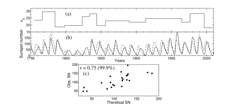
Figure 1: (a) Variation of amplitudes of meridional circulation $v_{0}$ (in m s^-1) with time (in yr). The solid line is the variation of $v_{0}$ used to match the theoretical periods with the observed periods. (b) Variation of theoretical sunspot number (dashed line) and observed sunspot number (solid line) with time. (c) Scatter diagram showing peak theoretical sunspot number and peak observed sunspot number. The linear correlation coefficients and the corresponding significance levels are given on the plot.

In Fig. 1(b), we show the theoretical sunspot series (eruptions) by dashed line along with the observed sunspot series by solid line. The theoretical sunspot series has been multiplied by a factor to match the observed value. It is very interesting to see that most of the amplitudes of the theoretical sunspot cycle have been matched with the observed sunspot cycle. Therefore, we have found a significant correlation between these two (see Fig. 1(c)). This study suggests that a major part of the fluctuations of the amplitude of the solar cycle may come from the fluctuations of the meridional circulation. This is a very important result of this analysis.

Now we explain the physics of this result based on Yeates et al. (2008). Toroidal field in the flux transport model, is generated by the stretching of the poloidal field in the tachocline. The production of this toroidal field is more if the poloidal field remains in the tachocline for longer time and vice versa. However, the poloidal field diffuses during its transport through the convection zone. As a result, if the diffusivity is very high, then much of the poloidal field diffuses away and very less amount of it reaches the tachocline to induct toroidal field. Therefore, when we decrease $v_{0}$ in high diffusivity model to match the period of a longer cycle, the poloidal field gets more time to diffuse during its transport through the convection zone. This ultimately leads to a lesser generation of toroidal field and hence the cycle becomes weaker. On the other hand, when we increase the value of $v_{0}$ to match the period of a shorter cycle, the poloidal field does not get much time to diffuse in the convection zone. Hence it produces stronger toroidal field and the cycle becomes stronger. Consequently, we get weaker amplitudes for longer periods and vice versa. However, this is not the case in low diffusivity model because in this model the diffusive decay of the fields are not much important. As a result, the slower meridional circulation means that the poloidal field remains in the tachocline for longer time and therefore it produces more toroidal field, giving rise to a strong cycle. Therefore, we do not get a correct correlation between the amplitudes of theoretical sunspot number and that of observed sunspot number when repeat the same analysis in low diffusivity model based on Dikpati & Charbonneau (1999) model.

2.2 Modeling Waldmeier effect

We study the Waldmeier effect using flux transport dynamo model. We have seen that the stochastic fluctuations in the Babcock–Leighton process and the stochastic fluctuations in the meridional circulation are the two main sources of irregularities in this model. Therefore, to study Waldmeier effect we first introduce suitable stochastic fluctuations in the poloidal field source term of Babcock–Leighton process. We see that this study cannot reproduce WE1 (Fig. 2(a)). However it reproduces WE2 (Fig. 2(b)).

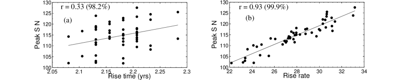
Figure 2: Theoretical plots of WE1 (a) and WE2 (b) obtained by introducing fluctuations in the poloidal field at the minima.

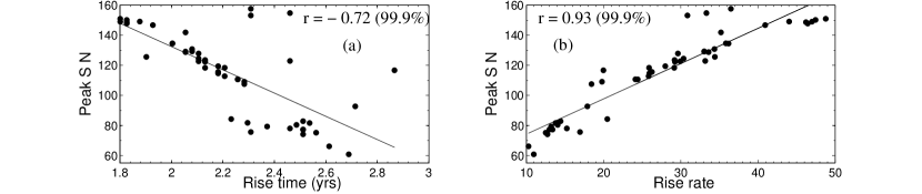
Figure 3: Theoretical plots of WE1 and WE2 obtained by introducing fluctuations in the meridional circulation.

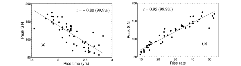
Figure 4: Theoretical plots of WE1 and WE2 obtained by introducing fluctuations in both the poloidal field generation and the meridional circulation.

Next we introduce stochastic fluctuations in the meridional circulation. Fig. 3 shows this result. Interestingly, we see that it reproduces not only WE2, but also WE1 (see Fig. 3(a)).

Finally we introduce stochastic fluctuations in both the poloidal field source term and the meridional circulation. We see that both WE1 and WE2 are remarkably reproduced in this case (see Fig. 4). We repeat the same study in low diffusivity model based on Dikpati & Charbonneau (1999) model. However in this case we are failed to reproduce WE1, only WE2 is reproduced. The details of this work can be found in Karak & Choudhuri (2011).

2.3 Modeling Maunder-like grand minimum

We have realized that the meridional circulation is important in modeling many aspects of solar cycle. Therefore we check whether a large decrease of the meridional circulation leads to a Maunder-like grand minimum. To answer this question, we decrease $v_{0}$ to a very low value in both the hemispheres. We have done this in the decaying phase of the last sunspot cycle before Maunder minimum. We keep $v_{0}$ at low value for around 1 yr and then we again increase it to the usual value but at different rates in two hemispheres. In northern hemisphere, $v_{0}$ is increased at slightly lower rate than southern hemisphere.

Figure 5: (a) The solid and dashed line show the variations of $v_{0}$ (in m s^-1) in northern and southern hemispheres with time. (b) The butterfly diagram. (c) The dashed and dotted lines show the sunspot numbers in southern and northern hemispheres, whereas the solid line is the total sunspot number. (d) Variation of energy density of toroidal field at latitude 15^∘ at the bottom of the convection zone.

In Fig. 5, we show the theoretical results covering the Maunder minimum episode. Fig. 5(a), shows the maximum amplitude of meridional circulation $v_{0}$ varied over this period in two hemispheres. In Fig. 5(b), we show the butterfly diagram of sunspot numbers, whereas in Fig. 5(c), we show the variation of total sunspot number along with the individual sunspot numbers in two hemispheres (see the caption). In order to facilitate comparison with observational data, we have taken the beginning of the year to be 1635. Note that our theoretical results reproduce the sudden initiation and the gradual recovery, the North-South asymmetry of sunspot number observed in the last phase of Maunder minimum and the cyclic oscillation of solar cycle found in cosmogenic isotope data.

We also mention that if we reduce the poloidal field to a very low value at the beginning of the Maunder minimum then also we can reproduce Maunder-like grand minimum (Choudhuri & Karak 2009). However in both the cases, either we need to reduce the meridional circulation or the poloidal field at the beginning of the Maunder minimum. However if we reduce the poloidal field little bit, then one can reproduce Maunder-like grand minimum at a moderate value of meridional circulation. The details of this study can be found in Karak (2010).

We have shown that with a suitable stochastic fluctuations in the meridional circulation, we are able to reproduce many important irregular features of solar cycle including Waldmeier effect and Maunder like grand minimum. However we are failed to reproduce these results in low diffusivity model. Therefore this study along with some earlier studies (Chatterjee, Nandy & Choudhuri 2004; Chatterjee & Choudhuri 2006; Goel & Choudhuri 2009; Jiang, Chatterjee & Choudhuri 2007; Karak 2010; Karak & Choudhuri 2011; Karak & Choudhuri 2012) supports the high diffusivity model for solar cycle.

Acknowledgements: I thank Prof. Arnab Rai Choudhuri for stimulating discussion and suggestion. I also thank the conference organizers for giving me the opportunity to present my work.

References

- (1) Chatterjee, P., Nandy, D., & Choudhuri, A. R. 2004, A&A, 427, 1019
- (2) Choudhuri, A. R., Chatterjee, P., & Jiang, J., 2007, Phys. Rev. Lett., 98, 1103
- (3) Choudhuri, A. R., & Karak, B. B. 2009, RAA 9, 953
- (4) Choudhuri, A. R., Schüssler, M., & Dikpati, M. 1995, A&A, 303, L29
- (5) Dikpati, M., & Charbonneau, P. 1999, ApJ, 518, 508
- (6) Jiang, J., Chatterjee, P., & Choudhuri, A. R. 2007, MNRAS, 381, 1527
- (7) Hoyt, D. V., & Schatten, K. H., 1996, Sol. Phys., 165, 181
- (8) Karak, B. B. 2010, ApJ, 724, 1021
- (9) Karak, B. B., & Choudhuri, A. R. 2011, MNRAS, 410, 1503
- (10) Karak, B. B., & Choudhuri, A. R. 2012, Sol. Phys., 278:137
- (11) Usoskin, I. G., Solanki, S. K., & Kovaltsov, G. A. 2007, A&A, 471, 301
- (12) Yeates, A. R., Nandy, D., & Mackay, D. H. 2008, ApJ, 673, 544