Interacting viscous matter with a dark energy fluid

Abstract

We study a cosmological model composed of a dark energy fluid interacting with a viscous matter fluid in a spatially flat Universe. The matter component represents the baryon and dark matter and it is taken into account, through a bulk viscosity, the irreversible process that the matter fluid undergoes because of the accelerated expansion of the universe. The bulk viscous coefficient is assumed to be proportional to the Hubble parameter. The radiation component is also taken into account in the model. The model is constrained using the type Ia supernova observations, the shift parameter of the CMB, the acoustic peak of the BAO and the Hubble expansion rate, to constrain the values of the barotropic index of dark energy and the bulk viscous coefficient. It is found that the bulk viscosity is constrained to be negligible (around zero) from the observations and that the barotropic index for the dark energy to be negative and close to zero too, indicating a phantom energy.

1 Introduction

In the last years, the type Ia supernovae (SNe Ia) observations have given a strong evidence of a present accelerated expansion epoch of the Universe (see for instance Riess et al. (1998); Perlmutter et al. (1999); Amanullah et al. (2010) and references therein).

Several models have been proposed to explain this recent acceleration, one of the most successful one is the so-called $\Lambda$ Cold Dark Matter ($\Lambda$CDM) that proposes the existence of a new kind of component in the Universe called “dark energy” with a behavior of a cosmological constant and that constitutes $\sim 73\%$ of the total content of matter-energy in the Universe today, in addition to a dark matter component filling the Universe in a $\sim 23\%$ Amanullah et al. (2010).

However, this model faces several strong problems, one of them is the huge discrepancy between its predicted and observed value for the dark energy density (of about 120 orders of magnitude) Weinberg (1989); Padmanabhan (2003); Carroll (2001), another one is the so-called the “cosmic coincidence problem”: the model predicts that we are living in a moment when the matter density in the universe is of the same order of magnitude than the dark energy density Steinhardt et al. (1999).

On the other hand, cosmological models with interacting dark components have been studied by several authors, because it is expected that the two dominant components (dark energy and matter) interact each other in some way. It has been found that these models are promising mechanisms to solve the $\Lambda$CDM problems (see Chimento et al. (2000); Kremer and Sobreiro (2011) and references therein).

In addition, it has been known since several years ago before the discovery of the present acceleration that a bulk viscous fluid can produce an accelerating cosmology (although it was originally proposed in the context of an inflationary period in the early universe) Heller and Klimek (1975); Barrow (1986); Padmanabhan and Chitre (1987); Gron (1990); Maartens (1995); Zimdahl (1996).

So, it is natural to think of the bulk viscous pressure as one of the possible mechanism that can accelerate the universe today (see for instance Cataldo et al. (2005); Colistete et al. (2007); Avelino and Nucamendi (2009, 2010); Hipólito-Ricaldi et al. (2010); Montiel and Breton (2011)). However, this idea faces the problem of that it is necessary to propose a viable mechanism for the origin of the bulk viscosity, although in this sense some proposals have been already suggested Zimdahl (2000); Mathews et al. (2008).

In the present work, following the idea of Kremer et al (2011) Kremer and Sobreiro (2011) and using the SNe Ia, the shift parameter $R$ of the cosmic microwave background radiation (CMB), the baryon acoustic oscillation (BAO) and the Hubble expansion rate $H(z)$ data, we test an interacting dark sector model taking into account dissipative process through a bulk viscosity in the matter (baryon and dark matter) component, where the interaction term is written in terms of the barotropic index of the dark energy fluid.

In section 1 we present the characteristics of the model and the main equations, in section 2 we explain the cosmological probes used to constrain the model and in section 3 we give our conclusions.

2 Interacting dark fluids with bulk viscosity

We study a cosmological model in a spatially flat FRW universe, composed of three fluids: radiation, matter and a dark energy fluid components. It is assumed the matter component as a pressureless fluid, representing the baryon and dark matter, with a bulk viscosity and interacting with the dark energy fluid.

The Friedmann constraint and the conservation equations can be written as

$$H^{2} =\frac{8\pi G}{3}\left(\rho_{\rm r}+\rho_{\rm m}+\rho_{\rm de}\right),$$ (1)

$$0 =\dot{\rho}_{\rm r}+4H\rho_{\rm r},$$ (2)

$$0 =\dot{\rho}_{\rm m}+\dot{\rho}_{\rm de}+3H\left(\rho_{\rm m}+\rho_{\rm de}+p_{\rm m}+p_{\rm de}-3H\zeta\right),$$ (3)

where $(\rho_{\rm r},\rho_{\rm m},\rho_{\rm de})$ are the densities of the radiation, matter and dark fluid components respectively, and $(p_{\rm r},p_{\rm m},p_{\rm de})$ are their corresponding pressures. The equation (3) arises from assuming the interaction between the matter and dark fluid components. The term $-3H\zeta$ corresponds to the bulk viscous pressure of the matter fluid, where $\zeta$ is the bulk viscous coefficient.

The immediate solution of the conservation equation (2) is

$$\rho_{\rm r}(a)=\rho_{\rm r0}/a^{4},$$ (4)

where $a$ is the scale factor and the subscript zero labels the present values for the densities.

On the other hand, following the idea of Kremer and Sobreiro Kremer and Sobreiro (2011), the conservation equation (3) can be decoupled as

$$\dot{\rho}_{\rm m}+3H\gamma^{e}_{\rm m}\rho_{\rm m}=0,$$ (5)

$$\dot{\rho}_{\rm de}+3H\gamma^{e}_{\rm de}\rho_{\rm de}=0,$$ (6)

where it was defined the effective barotropic indexes $\gamma^{e}_{\rm m}$ and $\gamma^{e}_{\rm de}$ so that they are related as

$$\gamma^{e}_{\rm m}=\gamma_{\rm m}+\frac{\gamma_{\rm de}-\gamma^{e}_{\rm de}}{r}-\frac{3H\zeta}{\rho_{\rm m}},$$ (7)

with $r\equiv\rho_{\rm m}/\rho_{\rm de}$ corresponds to the ratio between the matter to dark energy densities and $p_{i}=(\gamma_{i}-1)\rho_{i}$ with $\gamma_{i}$ is the usual constant barotropic indexes of the equation of state.

We consider a bulk viscous coefficient $\zeta$ proportional to the total matter-energy density $\rho_{\rm t}=\rho_{\rm r}+\rho_{\rm m}+\rho_{\rm de}$, as

$$\zeta=\frac{\zeta_{0}}{\sqrt{24\pi G}}\rho^{1/2}_{\rm t},$$ (8)

with $\zeta_{0}$ a dimensionless constant. This parametrization corresponds to a bulk viscosity proportional to the expansion rate of the Universe, i.e., to the Hubble parameter [see eq. (1)].

Following Kremer and Sobreiro (2011) and Chimento et al. (2009), we assume that the effective barotropic index for the dark energy is given as

$$\gamma^{e}_{\rm de}=\gamma_{\rm de}+\zeta_{0}.$$ (9)

So, using (7) and (9), the effective conservation equations (5) and (6) can be rewritten as

$$\dot{\rho}_{\rm m}+3H\gamma_{\rm m}\rho_{\rm m} =3H\rho_{\rm de}\zeta_{0}+9H^{2}\zeta,$$ (10)

$$\dot{\rho}_{\rm de}+3H\gamma_{\rm de}\rho_{\rm de} =-3H\rho_{\rm de}\zeta_{0},$$ (11)

where it can be identified the interacting term $Q\equiv 3H\rho_{\rm de}\zeta_{0}$.

Using the expression (9), the solution of the conservation equation (6) becomes

$$\rho_{\rm de}(a)=\rho_{\rm de0}/a^{3(\gamma_{\rm de}+\zeta_{0})}.$$ (12)

On the other hand, with the eqs. (8) and (9) we can express the equation (7) as

$$\gamma^{e}_{\rm m}=\gamma_{\rm m}-\frac{\zeta_{0}}{\rho_{\rm m}}\left(\rho_{\rm de}+\frac{3H^{2}}{8\pi G}\right),$$ (13)

that using the Friedmann constraint (1) we arrive to

$$\gamma^{e}_{\rm m}=\gamma_{\rm m}-\frac{\zeta_{0}}{\rho_{\rm m}}\left(\rho_{\rm r}+\rho_{\rm m}+2\rho_{\rm de}\right).$$ (14)

Inserting the eqs. (4) and (12) at (14) we obtain

$$\gamma^{e}_{\rm m}=\gamma_{\rm m}-\frac{\zeta_{0}}{\rho_{\rm m}}\left(\frac{\rho_{\rm r0}}{a^{4}}+2\frac{\rho_{\rm de0}}{a^{3(\gamma_{\rm de}+\zeta_{0})}}+\rho_{\rm m}\right).$$ (15)

With this, the eq. (6) for the matter density becomes

$$\dot{\rho}_{\rm m}+3H\gamma_{\rm m}\rho_{\rm m}-3H\zeta\left(\frac{\rho_{\rm r0}}{a^{4}}+2\frac{\rho_{\rm de0}}{a^{3(\gamma_{\rm de}+\zeta_{0})}}+\rho_{\rm m}\right)=0.$$ (16)

Dividing to (16) by the present critical density $\rho_{\rm crit}^{0}\equiv 3H^{2}_{0}/(8\pi G)$ with $H_{0}$ the Hubble constant, and defining the dimensionless parameter densities $\Omega_{i0}\equiv\rho_{i0}/\rho^{0}_{\rm crit}$, the eq. (16) becomes

$$\frac{d\hat{\Omega}_{\rm m}}{da}+\frac{3}{a}\left[\hat{\Omega}_{\rm m}(\gamma_{\rm m}-\zeta_{0})-\zeta_{0}\left(\frac{\Omega_{\rm r0}}{a^{4}}+\frac{2\Omega_{\rm de0}}{a^{3(\gamma_{\rm de}+\zeta_{0})}}\right)\right]=0,$$ (17)

or in terms of the redshift $z$ with the help of the relation $a=1/(1+z)$,

$$(1+z)\frac{d\hat{\Omega}_{\rm m}}{dz}-3\left[\hat{\Omega}_{\rm m}(\gamma_{\rm m}-\zeta_{0})-\zeta_{0}\left(\Omega_{\rm r0}(1+z)^{4}+2\Omega_{\rm de0}(1+z)^{3(\gamma_{\rm de}+\zeta_{0})}\right)\right]=0,$$ (18)

where it has been defined $\hat{\Omega}_{\rm m}\equiv\rho_{\rm m}/\rho^{0}_{\rm crit}$. The analytical solution of this ordinary differential equation (ODE) for $\hat{\Omega}_{\rm m}(z)$ is

$$\hat{\Omega}_{\rm m}(z)= [(1+z)^{-3\zeta_{0}}[2(1+z)^{3(\gamma_{\rm de}+2\zeta_{0})}\zeta_{0}(4-3\gamma_{\rm m}+3\zeta_{0})(\Omega_{\rm m0}+\Omega_{\rm r0}-1)-$$ (19)

$$-3(1+z)^{4+3\zeta_{0}}\zeta_{0}(\gamma_{\rm de}-\gamma_{\rm m}+2\zeta_{0})\Omega_{\rm r0}+$$

$$(1+z)^{3\gamma_{\rm m}}((4-3\gamma_{\rm m}+3\zeta_{0})(2\zeta_{0}+(\gamma_{\rm de}-\gamma_{\rm m})\Omega_{\rm m0})+$$

$$+(3\gamma_{\rm de}+3\gamma_{\rm m}-8)\zeta_{0}\Omega_{\rm r0})]]/$$

$$\left((\gamma_{\rm de}-\gamma_{\rm m}+2\zeta_{0})(4-3\gamma_{\rm m}+3\zeta_{0})\right).$$

So, using the solution (19), the Hubble parameter (1) can be written as

$$E^{2}(z)=\Omega_{\rm r0}(1+z)^{4}+\Omega_{\rm de0}(1+z)^{3(\gamma_{\rm de}+\zeta_{0})}+\hat{\Omega}_{\rm m}(z),$$ (20)

where $E(z)\equiv H(z)/H_{0}$. In the following we will assume $\gamma_{\rm m}=0$, i.e., the matter as a pressureless fluid.

3 Cosmological probes

We compare the model with the following cosmological probes that measure the expansion history of the Universe, to constrain the values of $(\zeta_{0},\gamma_{\rm de})$.

3.0.1 Type Ia Supernovae

We use the type Ia supernovae (SNe Ia) of the “Union2” data set (2010) from the Supernova Cosmology Project (SCP) composed of 557 SNe Ia Amanullah et al. (2010). The luminosity distance $d_{L}$ in a spatially flat Universe is defined as

$$d_{L}(z,\zeta_{0},\gamma_{\rm de},H_{0})=\frac{c(1+z)}{H_{0}}\int_{0}^{z}\frac{dz^{\prime}}{E(z^{\prime},\zeta_{0},\gamma_{\rm de})},$$ (21)

where “$c$” corresponds to the speed of light in units of km/sec. The theoretical distance moduli $\mu^{t}$ for the k-th supernova at a distance $z_{k}$ given by

$$\mu^{t}(z,\zeta_{0},\gamma_{\rm de},H_{0})=5\log\left[\frac{d_{L}(z,\zeta_{0},\gamma_{\rm de},H_{0})}{\rm Mpc}\right]+25.$$ (22)

So, the $\chi^{2}$ function is defined as

$$\chi^{2}_{\rm SNe}(\zeta_{0},\gamma_{\rm de},H_{0})\equiv\sum_{k=1}^{n}\left(\frac{\mu^{t}(z_{k},\zeta_{0},\gamma_{\rm de},H_{0})-\mu_{k}}{\sigm ạ_{k}}\right)^{2},$$ (23)

where $\mu_{k}$ is the observed distance moduli of the k-th supernova, with a standard deviation of $\sigm ạ_{k}$ in its measurement, and $n=557$.

3.0.2 Cosmic Microwave Background Radiation

We use the WMAP 7-years distance priors release shown in table 9 of Komatsu et al. (2011), composed of the shift parameter $R$, the acoustic scale $l_{A}$ and the redshift of decoupling $z_{*}$.

The shift parameter $R$ is defined as

$$R=H_{0}\frac{\sqrt{\Omega_{\rm m0}}}{c}(1+z_{*})D_{A}(z_{*}),$$ (24)

where $D_{A}$ is the proper angular diameter distance given by (for a spatially flat Universe)

$$D_{A}(z)=\frac{c}{(1+z)H_{0}}\int^{z}_{0}\frac{dz^{\prime}}{E(z^{\prime},\zeta_{0},\gamma_{\rm de})}.$$ (25)

With $R$ we can defined a $\chi^{2}$ function as

$$\chi^{2}_{\rm R-CMB}(\zeta_{0},\gamma_{\rm de},H_{0})\equiv\left(\frac{R(\zeta_{0},\gamma_{\rm de},H_{0})-R_{\rm obs}}{\sigma_{R}}\right)^{2},$$ (26)

where $R_{\rm obs}=1.725$ is the “observed” value of the shift parameter and $\sigma_{R}=0.018$ the standard deviation of the measurement (cf. table 9 of Komatsu et al. (2011)).

The acoustic scale $l_{A}$ is defined as

$$l_{A}\equiv(1+z_{*})\frac{\pi D_{A}(z_{*})}{r_{s}(z_{*})},$$ (27)

where $r_{s}(z_{*})$ corresponds to the comoving sound horizon at the decoupling epoch of photons, $z_{*}$, given by

$$r_{s}(z)=\frac{c}{\sqrt{3}}\int_{0}^{1/(1+z)}\frac{da}{a^{2}H(a)\sqrt{1+(3\Omega_{\rm b0}/4\Omega_{\gamma 0})a}},$$ (28)

where we use $\Omega_{\gamma 0}=2.469\times 10^{-5}h^{-2}$ the radiation, and $\Omega_{\rm b0}=0.02255h^{-2}$ the baryon matter component, as reported by Komatsu et al. 2010 Komatsu et al. (2011). For $z_{*}$ we use the fitting formula proposed by Hu and Sugiyama Hu and Sugiyama (1996)

$$z_{*}=1048\left[1+0.00124(\Omega_{\rm b0}h^{2})^{-0.738}\right]\left[1+g_{1}(\Omega_{\rm m0}h^{2})^{g_{2}}\right],$$ (29)

where

$$g_{1}=\frac{0.0783(\Omega_{\rm b0}h^{2})^{-0.238}}{1+39.5(\Omega_{\rm b0}h^{2})^{0.763}},\;\;\;\;\;g_{2}=\frac{0.560}{1+21.1(\Omega_{\rm b0}h^{2})^{1.81}}.$$ (30)

The $\chi^{2}$ function using the three values $(l_{A},R,z_{*})$ is defined as

$$\chi^{2}_{\rm CMB}(\zeta_{0},\gamma_{\rm de},H_{0})=\sum_{i,j=1}^{3}(x_{i}-d_{i})(C^{-1})_{ij}(x_{j}-d_{j}),$$ (31)

where $x_{i}\equiv(l_{A},R,z_{*})$ are the predicted values by the model and $d_{i}\equiv(l_{A}=302.09,R=1.725,z_{*}=1091.3)$ are the observed ones and $C^{-1}_{ij}$ is the inverse covariance matrix Komatsu et al. (2011)

$$C^{-1}=\begin{pmatrix}2.305&29.698&-1.333\\ 29.698&6825.27&-113.180\\ 1.333&113.180&3.414\end{pmatrix}.$$ (32)

3.0.3 Baryon Acoustic Oscillations

We use the baryon acoustic oscillation (BAO) data from the SDSS 7-years release Percival et al. (2010). The distance ratio $d_{z}$ at $z=0.275$ is defined as

$$d_{0.275}\equiv\frac{r_{s}(z_{d})}{D_{V}(0.275)},$$ (33)

where $z_{d}$ is the redshift at the baryon drag epoch computed from the following fitting formula Eisenstein and Hu (1998)

$$z_{d} =1291\frac{(\Omega_{m0}h^{2})^{0.251}}{1+0.659(\Omega_{m0}h^{2})^{0.828}}\left[1+b_{1}(\Omega_{m0}h^{2})^{b_{2}}\right],$$ (34)

$$b_{1} =0.313(\Omega_{m0}h^{2})^{-0.419}\left[1+0.607(\Omega_{m0}h^{2})^{0.674}\right],$$ (35)

$$b_{2} =0.238(\Omega_{m0}h^{2})^{0.223}.$$ (36)

For a flat Universe, $D_{V}(z)$ is defined as

$$D_{V}(z)=c\left[\left(\int_{0}^{z}\frac{dz^{\prime}}{H(z^{\prime})}\right)^{2}\frac{z}{H(z)}\right]^{1/3},$$ (37)

contains the information of the visual distortion of a spherical object due the non Euclidianity of the FRW spacetime.

The $d_{0.275}$ contains the information of the other two pivots, $d_{0.2}$ and $d_{0.35}$ usually used for other authors, with a precision of $0.04\%$ Percival et al. (2010).

The $\chi^{2}$ function for BAO is defined as

$$\chi^{2}_{\rm BAO}(\zeta_{0},\gamma_{\rm de},H_{0})\equiv\left(\frac{d_{0.275}-d_{0.275}^{\rm obs}}{\sigma_{d}}\right)^{2},$$ (38)

where $d_{0.275}^{\rm obs}=0.139$ is the “observed” value and $\sigma_{d}=0.0037$ the standard deviation of the measurement Percival et al. (2010).

3.0.4 Hubble expansion rate

For the Hubble parameter we use 13 available data, 11 comes from the table 2 of Stern et al. (2010) Stern et al. (2010) and the 2 following data from Gaztanaga et al. 2010 Gaztanaga et al. (2009): $H(z=0.24)=79.69\pm 2.32$ and $H(z=0.43)=86.45\pm 3.27$ km/s/Mpc. For the present value of the Hubble parameter we take that reported by Riess et al 2011 Riess et al. (2011) $H(z=0)\equiv H_{0}=73.8\pm 2.4$ km/s/Mpc. The $\chi^{2}$ function is defined as

$$\chi^{2}_{\rm H}(\zeta_{0},\gamma_{\rm de},H_{0})=\sum_{i}^{13}\left(\frac{H(z_{i},\zeta_{0},\gamma_{\rm de})-H_{i}^{\rm obs}}{\sigma_{H}}\right)^{2},$$ (39)

where $H(z_{i})$ is the theoretical value predicted by the model and $H_{i}^{\rm obs}$ is the observed value.

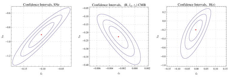
Figure 1: Confidence intervals for $(\zeta_{0},\gamma_{\rm de})$. The left panel corresponds to the constraint using the SNe Ia “Union2” data set. The central panel, using the $(R,l_{A},z_{*})$ data from the CMB and the left panel to the Hubble parameter $H(z)$. It was assumed a value of $H_{0}=73.8$ km/s/Mpc as suggested by Riess et al. (2011). The best estimated values and the $\chi^{2}$ minimum values are shown in table 1. The contours correspond to 63.8%, 95% and 99% of confidence level.

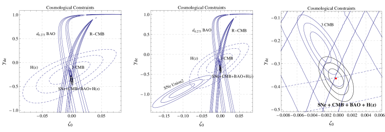
Figure 2: Confidence intervals (CI) together for $(\zeta_{0},\gamma_{\rm de})$. They correspond to the constraints when it is used the SNe Ia dataset, the $d_{0.275}$ BAO probe (see eq. [38]), the shift parameter $R$ of the CMB (see eq. [26]), the three $(R,l_{A},z_{*})$ data from the CMB (see eq. [31]), the Hubble parameter $H(z)$ (see eq. [39]), and the joint “SNe + CMB + BAO + $H(z)$” (black contours). It was assumed a value of $H_{0}=73.8$ km/s/Mpc as suggested by Riess et al. (2011). The contours correspond to 63.8%, 95% and 99% of confidence level.

3.0.5 Local Second Law of Thermodynamics

The law of generation of local entropy in a fluid on a FRW space–time can be written as Weinberg (1972); Misner and Wheeler (1973)

$$T\,\nabla_{\nu}s^{\nu}=\zeta(\nabla_{\nu}u^{\nu})^{2}=9H^{2}\zeta,$$ (40)

where $T$ is the temperature and $\nabla_{\nu}s^{\nu}$ is the rate of entropy production in a unit volume. With this, the second law of the thermodynamics can be written as

$$T\nabla_{\nu}s^{\nu}\geq 0,$$ (41)

so, from the expression (40), it simply implies that $\zeta\geq 0$.

For the present model this inequality becomes (see eq. [8])

$$\zeta_{0}\geq 0.$$ (42)

Probe	$\zeta_{0}$	$\gamma_{\rm de}$	$\chi^{2}_{{\rm min}}$	$\chi^{2}_{{\rm d.o.f.}}$
SNe Ia	$-0.102\pm 0.022$	$-0.904\pm 0.11$	$590.69$	1.06
$(R,l_{A},z_{*})$ CMB	$-0.0025\pm 0.001$	$-0.226\pm 0.04$	1.01	1.01
$H(z)$	$-0.003\pm 0.022$	$-0.199^{+0.14}_{-0.16}$	$8.049$	$0.731$
SNe Ia + CMB + BAO + $H(z)$	$-0.00035\pm 0.0007$	$-0.363\pm 0.028$	635.78	1.06

Table 1: Best estimated values of the dimensionless coefficients $\zeta_{0}$ and $\gamma_{\rm de}$. Figures 1 and 2 show the confidence intervals.

4 Conclusions

It has been studied a cosmological model composed of a bulk viscous matter fluid interacting with a dark energy fluid. The model is compared with cosmological observations to estimate and constrain the values of the bulk viscous coefficient $\zeta_{0}$ proportional to the Hubble parameter, and the barotropic index of the dark energy $\gamma_{\rm de}$. It is also used the local second law of thermodynamics (LSLT), that states $\zeta_{0}>0$, as a criterion for the allowed values for $\zeta_{0}$.

It is found that using the combined SNe + CMB + BAO + $H(z)$ data sets, the best estimated value of $\zeta_{0}$ is negative (implying a violation of the LSLT) and very close to zero. The confidence intervals constrain the values of $\zeta_{0}$ to be very around to zero, $-0.003<\zeta_{0}<0.0025$, with a 99% of confidence level. We interpret these results as an indication that the cosmological data prefer a model with a practically null bulk viscosity. Since in the present model the interacting term is proportional to the bulk viscosity, this implies also a negligible interaction between the dark components.

On the other hand, it is found negatives values of $\gamma_{\rm de}$ with a 99% of confidence level, corresponding to a phantom dark energy.

It may be an indicative of the phantom energy as a preferred mechanism by the cosmological observations (in combination with the LSLT) to explain the accelerated expansion of the Universe, instead of the bulk viscous mechanism.

References

• Riess et al. (1998) A. G. Riess, et al., Astron.J. 116, 1009–1038 (1998), astro-ph/9805201.
• Perlmutter et al. (1999) S. Perlmutter, et al., Astrophys.J. 517, 565–586 (1999), the Supernova Cosmology Project, astro-ph/9812133.
• Amanullah et al. (2010) R. Amanullah, C. Lidman, D. Rubin, G. Aldering, P. Astier, et al., Astrophys.J. 716, 712–738 (2010), 1004.1711.
• Weinberg (1989) S. Weinberg, Rev. Mod. Phys. 61, 1–23 (1989), URL http://link.aps.org/doi/10.1103/RevModPhys.61.1.
• Padmanabhan (2003) T. Padmanabhan, Phys.Rept. 380, 235–320 (2003), hep-th/0212290.
• Carroll (2001) S. M. Carroll, Living Rev.Rel. 4, 1 (2001), astro-ph/0004075.
• Steinhardt et al. (1999) P. J. Steinhardt, L.-M. Wang, and I. Zlatev, Phys.Rev. D59, 123504 (1999), astro-ph/9812313.
• Chimento et al. (2000) L. P. Chimento, A. S. Jakubi, and D. Pavón, Phys. Rev. D 62, 063508 (2000), URL http://link.aps.org/doi/10.1103/PhysRevD.62.063508.
• Kremer and Sobreiro (2011) G. M. Kremer, and O. A. Sobreiro (2011), 1109.5068.
• Heller and Klimek (1975) M. Heller, and Z. Klimek, Astrophysics and Space Science 33, L37–L39 (1975).
• Barrow (1986) J. D. Barrow, Physics Letters B 180, 335–339 (1986), ISSN 0370-2693, URL http://www.sciencedirect.com/science/article/pii/037026938691%1986.
• Padmanabhan and Chitre (1987) T. Padmanabhan, and S. Chitre, Physics Letters A 120, 433–436 (1987), ISSN 0375-9601, URL http://www.sciencedirect.com/science/article/pii/037596018790%1046.
• Gron (1990) O. Gron, Astrophys. Space Sci. 173, 191–225 (1990).
• Maartens (1995) R. Maartens, Classical and Quantum Gravity 12, 1455 (1995), URL http://stacks.iop.org/0264-9381/12/i=6/a=011.
• Zimdahl (1996) W. Zimdahl, Phys. Rev. D 53, 5483–5493 (1996), URL http://link.aps.org/doi/10.1103/PhysRevD.53.5483.
• Cataldo et al. (2005) M. Cataldo, N. Cruz, and S. Lepe, Phys.Lett. B619, 5–10 (2005), hep-th/0506153.
• Colistete et al. (2007) R. Colistete, J. Fabris, J. Tossa, and W. Zimdahl, Phys.Rev. D76, 103516 (2007), 0706.4086.
• Avelino and Nucamendi (2009) A. Avelino, and U. Nucamendi, JCAP 0904, 006 (2009), 0811.3253.
• Avelino and Nucamendi (2010) A. Avelino, and U. Nucamendi, JCAP 1008, 009 (2010), 1002.3605.
• Hipólito-Ricaldi et al. (2010) W. S. Hipólito-Ricaldi, H. E. S. Velten, and W. Zimdahl, Phys. Rev. D 82, 063507 (2010), URL http://link.aps.org/doi/10.1103/PhysRevD.82.063507.
• Montiel and Breton (2011) A. Montiel, and N. Breton, JCAP 1108, 023 (2011), 1107.0271.
• Zimdahl (2000) W. Zimdahl, Phys.Rev. D61, 083511 (2000), astro-ph/9910483.
• Mathews et al. (2008) G. Mathews, N. Lan, and C. Kolda, Phys.Rev. D78, 043525 (2008), 0801.0853.
• Chimento et al. (2009) L. P. Chimento, M. I. Forte, and G. M. Kremer, Gen.Rel.Grav. 41, 1125–1137 (2009), 0711.2646.
• Komatsu et al. (2011) E. Komatsu, et al., Astrophys.J.Suppl. 192, 18 (2011), 1001.4538.
• Hu and Sugiyama (1996) W. Hu, and N. Sugiyama, Astrophys.J. 471, 542–570 (1996), revised version, astro-ph/9510117.
• Percival et al. (2010) W. J. Percival, et al., Mon.Not.Roy.Astron.Soc. 401, 2148–2168 (2010), 21 pages, 15 figures, 0907.1660.
• Eisenstein and Hu (1998) D. J. Eisenstein, and W. Hu, Astrophys.J. 496, 605 (1998), astro-ph/9709112.
• Stern et al. (2010) D. Stern, R. Jimenez, L. Verde, M. Kamionkowski, and S. A. Stanford, JCAP 1002, 008 (2010), 0907.3149.
• Gaztanaga et al. (2009) E. Gaztanaga, A. Cabre, and L. Hui, Mon.Not.Roy.Astron.Soc. 399, 1663–1680 (2009), 0807.3551.
• Riess et al. (2011) A. G. Riess, L. Macri, S. Casertano, H. Lampeitl, H. C. Ferguson, et al., Astrophys.J. 730, 119 (2011), 1103.2976.
• Weinberg (1972) S. Weinberg, Gravitation and Cosmology: principles and applications of the general theory of relativity, John Wiley & Sons Inc, New York, USA, 1972.
• Misner and Wheeler (1973) C. W. Misner, and J. A. Wheeler, Gravitation, W. H. Freeman and Company, USA, 1973.