Exact results with the Kotliar-Ruckenstein slave-boson representation

Abstract

Radial slave boson representations have the particular advantage that the expectation values of their respective fields are finite even without the formal introduction of spurious Bose condensates for each of the bosonic fields. The expectation values of the radial (real) fields are in fact to be interpreted as the density of empty or singly occupied sites. Whereas the radial representation of the Barnes slave bosons has been investigated before, a setup for the functional integral of radial bosonic fields in the more physical Kotliar-Ruckenstein representation has not been accomplished to date. We implement a path integral procedure with suitable renormalization factors for a strongly correlated two-site model which allows to control the formal steps in the intricate evaluation, as the results for the partition function and the expectation values are known from exact diagonalization for such a minimal single impurity Anderson model. The partition function is shown to be a trace over a product of matrices local in time and therefore can be calculated analytically. Eventually, we establish the scheme for the evaluation of correlation functions and thermodynamic properties.

1 Introduction

Application-oriented, fundamental properties of correlated electronic systems have become numerous in recent years, in particular for transition metal oxides: high-T_c superconductivity (see, e.g., [1, 2]), colossal magnetoresistance (see, e.g.,[3]), transparent conducting oxides (see, e.g.,[4]), high capacitance heterostructures [5] or large thermopower (see, e.g.,[6]), to quote a few. In addition, they also entail fascinating phenomena such as superconductivity at the interface of two insulators [7], peculiar magnetism in low dimensional systems [8], high temperature ferromagnetism in vanadate superlattices [9], all of them providing a strong challenge to investigate these systems from the theory side. Yet, it is fair to say that current theoretical approaches meet with severe difficulties when studying the models which describe these systems. Indeed, the tool, which is best mastered (perturbation theory), badly fails when the Coulomb interaction, both local and non-local, is sufficiently strong, thereby calling for alternative approaches. The introduction of generalized coherent states [10] in a constrained Fock space allows for the setup of a well-defined functional integral for strong Coulomb interaction [11] but these path integrals are difficult to handle on account of the non-trivial Berry phases. An appealing scheme, which is rather based on canonical fermionic and bosonic fields, the slave boson representation of local states, was introduced by Barnes to tackle the single impurity Anderson model (SIAM) [12]. Later the slave boson approach has been extended to a whole series of models [13, 14, 15, 16, 17, 18, 20, 21, 19] (for a review see [22]) .

Notably, Kroha et al. [23] developed a scheme which guarantees local gauge invariance in a conserving approximation and allows for Fermi liquid as well as non-Fermi liquid behavior for the investigated multi-channel Anderson impurity problem. In a different approach towards local gauge invariance, Read and Newns demonstrated that the phase of the slave boson field may be gauged away, at the price of introducing a time dependent constraint [24]. By doing so the slave boson is reduced to a radial slave boson field. Such fields do not possess dynamics on their own, but only through their coupling to the fermions. The radial representation has not been intensively investigated, and the corresponding literature mostly focuses on the Barnes representation of the SIAM [25, 26].

Besides, there seem to be (infinitely) many slave boson representations to a particular model. This has been shown to be of advantage by Kotliar and Ruckenstein when investigating the Hubbard model [14], as they devised their representation in such a way that the Gutzwiller approximation is recovered in a paramagnetic saddle-point approximation. This approach is exact in the large degeneracy limit [17, 27] and obeys a variational principle in the limit of large spatial dimensions where the Gutzwiller approximation and the Gutzwiller wave function are identical [28]. Extensions [16, 17, 18, 20] have been applied successfully to a number of problems [29, 30], all of them making use of a specific representation of the kinetic energy operator. As the suggested operator takes an involved form, which is only defined through a corresponding series expansion, it could not yet be proven to comply to the normal ordering procedure, and therefore deserves further study. This is the aim of this paper. The correctness of various representations of the kinetic energy operator and interaction terms will be judged by the exact evaluation of the resulting functional integral representation of the partition function. We then illustrate the calculation of the expectation value of the radial slave boson fields. Being intrinsically phase stiff these fields do not average to zero, in contrast to canonical bosonic fields. Therefore their finite expectation value is by no means related to a Bose condensate.

2 Gauge symmetry and radial slave boson representation

We investigate an exactly soluble model, the simplified single impurity Anderson model enriched by a non-local Coulomb interaction term. The hamiltonian reads:

$${\mathcal{H}}=\sum_{\sigma}\left(\epsilon_{\rm c}c^{\dagger}_{\sigma}c^{\phantom{\dagger}}_{\sigma}+\epsilon_{\rm a}a^{\dagger}_{\sigma}a^{\phantom{\dagger}}_{\sigma}+V\left(c^{\dagger}_{\sigma}a^{\phantom{\dagger}}_{\sigma}+{\rm h.c.}\right)\right)+Ua^{\dagger}_{\uparrow}a^{\phantom{\dagger}}_{\uparrow}a^{\dagger}_{\downarrow}a^{\phantom{\dagger}}_{\downarrow}+In_{\rm a}n_{\rm c}$$ (1)

which is defined on two sites. The one-body terms involve the operators $c^{\dagger}_{\sigma}$ ($c^{\phantom{\dagger}}_{\sigma}$) and $a^{\dagger}_{\sigma}$ ($a^{\phantom{\dagger}}_{\sigma}$). They represent the creation (annihilation) of “band” and “impurity” electrons, with spin projection $\sigma$. The energies $\epsilon_{\rm c}$ and $\epsilon_{\rm a}$ are the band and impurity energy levels, respectively, while the hybridization energy is $V$. Regarding the two-body terms, $I$ represents the non-local Coulomb interaction and $U$ is the on-site repulsion. It is the largest energy scale in the model and it will be set to infinity as in the standard infinite-$U$ SIAM. Standard perturbation theory in the interaction may not be considered for this problem. While this model may be solved by means of exact diagonalization [21], we here investigate it by means of a Kotliar and Ruckenstein slave boson representation. There, the local physical electron operator $a_{\sigma}$ for the impurity site is rewritten as a product of the auxiliary fermionic fields $f_{\sigma}$ and auxiliary bosonic fields $e$, $p_{\sigma}$ and $d$, representing the empty, singly occupied and the doubly occupied site, respectively. The partition function reads for $U\rightarrow\infty$:

$${\mathcal{Z}} = \int_{-\pi/\beta}^{\pi/\beta}\frac{\beta d\lambda^{(1)}}{2\pi}\prod_{\sigma}\int_{-\pi/\beta}^{\pi/\beta}\frac{\beta d\lambda^{(2)}_{\sigma}}{2\pi}\int\prod_{\sigma}D[c^{\phantom{\dagger}}_{\sigma},c^{\dagger}_{\sigma}]D[f^{\phantom{\dagger}}_{\sigma},f^{\dagger}_{\sigma}]\int D[e,e^{\dagger}]\int\prod_{\sigma}D[p^{\phantom{\dagger}}_{\sigma},p^{\dagger}_{\sigma}]$$ (2)

$$\times e^{-\int_{0}^{\beta}d\tau{\mathcal{L}}(\tau)}$$

with the Lagrangian

$${\mathcal{L}}(\tau)={\mathcal{L}}_{f}(\tau)+{\mathcal{L}}_{b}(\tau)+{\mathcal{L}}_{V}(\tau)+{\mathcal{L}}_{\mathnormal{I}}(\tau)$$ (3)

consisting of

$${\mathcal{L}}_{f}(\tau) = \sum_{\sigma}f^{\dagger}_{\sigma}(\tau)\left(\partial_{\tau}-\mu+i\lambda^{(2)}_{\sigma}\right)f^{\phantom{\dagger}}_{\sigma}(\tau)$$

$${\mathcal{L}}_{b}(\tau) = e^{\dagger}(\tau)\left(\partial_{\tau}+i\lambda^{(1)}\right)e(\tau)+\sum_{\sigma}p^{\dagger}_{\sigma}(\tau)\left(\partial_{\tau}+i\lambda^{(1)}-i\lambda^{(2)}_{\sigma}\right)p^{\phantom{\dagger}}_{\sigma}(\tau)-i\lambda^{(1)}$$

$${\mathcal{L}}_{V}(\tau) = V\sum_{\sigma}\left(e^{\dagger}(\tau)p^{\phantom{\dagger}}_{\sigma}(\tau)f^{\phantom{\dagger}}_{\sigma}(\tau)c^{\dagger}_{\sigma}(\tau)+e(\tau)p^{\dagger}_{\sigma}(\tau)f^{\dagger}_{\sigma}(\tau)c^{\phantom{\dagger}}_{\sigma}(\tau)\right)$$

$${\mathcal{L}}_{\mathnormal{I}}(\tau) = I\left(1-e^{\dagger}(\tau)e(\tau)\right)\sum_{\sigma}c^{\dagger}_{\sigma}(\tau)c^{\phantom{\dagger}}_{\sigma}(\tau)\;.$$ (4)

The first two contributions entail the dynamics of the auxiliary fields, together with the constraints, specific to the Kotliar and Ruckenstein setup. The hybridization and the non-local Coulomb interaction are represented by the last two terms. Here, the slave bosons $e$ ($p_{\sigma}$) refer to empty (singly occupied) sites, respectively. They are subject to the constraints

$$e^{\dagger}e+\sum_{\sigma}p^{\dagger}_{\sigma}p^{\phantom{\dagger}}_{\sigma} = 1$$

$$f^{\dagger}_{\sigma}f^{\phantom{\dagger}}_{\sigma}-p^{\dagger}_{\sigma}p^{\phantom{\dagger}}_{\sigma} = 0\;\;\;\;\;\;\;\;\;\;\sigma=\uparrow,\downarrow\;.$$ (5)

They are enforced by the Lagrange multipliers $\lambda^{(1)}$, resp. $\lambda^{(2)}_{\sigma}$. The Lagrangian, Eq. (3), possesses a $U(1)\times U(1)\times U(1)$ gauge symmetry group. Indeed, performing the gauge transformation of the fermionic fields

$$f^{\phantom{\dagger}}_{\sigma}(\tau)\longrightarrow e^{-i\chi_{\sigma}(\tau)}f^{\phantom{\dagger}}_{\sigma}(\tau)$$ (6)

and expressing the bosonic fields in amplitude and phase variables as

$$e(\tau) = \sqrt{R_{e}(\tau)}e^{i\theta(\tau)}$$

$$p^{\phantom{\dagger}}_{\sigma}(\tau) = \sqrt{R_{\sigma}(\tau)}e^{i(\chi_{\sigma}(\tau)+\theta(\tau))}$$ (7)

allows to gauge away the phases of the three slave boson fields provided one introduces the three time dependent constraints:

$$\alpha(\tau) \equiv i\left(\lambda^{(1)}+\partial_{\tau}\theta(\tau)\right)$$

$$\beta_{\sigma}(\tau) \equiv i\left(\lambda^{(2)}_{\sigma}-\partial_{\tau}\chi_{\sigma}(\tau)\right).$$ (8)

We here introduced the radial slave boson fields in the continuum limit following, e. g., Refs. [24]. When dealing with discretized time steps special care has to be taken. Extending the procedure introduced in Ref. [25] for Barnes slave bosons to the Kotliar and Ruckenstein representation one obtains the partition function as:

$${\mathcal{Z}} = \lim_{N\rightarrow\infty}\lim_{\eta\rightarrow 0^{+}}\lim_{\Omega\rightarrow\infty}\left(\prod_{n=1}^{N}\int_{-\Omega}^{\Omega}\frac{\delta d\alpha_{n}}{2\pi}\int_{-\Omega}^{\Omega}\frac{\delta d\beta_{\uparrow n}}{2\pi}\int_{-\Omega}^{\Omega}\frac{\delta d\beta_{\downarrow n}}{2\pi}\int_{-\eta}^{\infty}dR_{e,n}\int_{-\eta}^{\infty}dR_{\uparrow,n}\int_{-\eta}^{\infty}dR_{\downarrow,n}\right)$$ (9)

$$\times e^{-S_{b}}{\mathcal{Z}_{f}}$$

where $R_{e,n}$ ($R_{\sigma,n}$) corresponds to the amplitude of the above complex $e_{n}$ ($p_{\sigma,n}$) bosonic variable, $\delta\equiv\beta/N$, and

$$S_{b} = i\delta\sum_{n=1}^{N}\left[\alpha_{n}\left(R_{e,n}+R_{\uparrow,n}+R_{\downarrow,n}-1\right)-\sum_{\sigma}\beta_{\sigma n}R_{\sigma,n}\right]$$

$${\mathcal{Z}_{f}} = \int\prod_{\sigma}D[c^{\phantom{\dagger}}_{\sigma},c^{\dagger}_{\sigma}]D[f^{\phantom{\dagger}}_{\sigma},f^{\dagger}_{\sigma}]e^{-S_{f}}.$$ (10)

The fermionic contribution to the action is bi-linear in the fermionic fields. It is given by

$$S_{f} = \sum_{n=1}^{N}\sum_{\sigma}\left\{f^{\dagger}_{n,\sigma}\left[f_{n,\sigma}-f_{n-1,\sigma}\left[1-\delta\left(\epsilon_{\rm a}+i\beta_{\sigma n}-\mu\right)\right]\right]\right.$$ (11)

$$\left.+c^{\dagger}_{n,\sigma}\left[c_{n,\sigma}-c_{n-1,\sigma}\left[1-\delta\left(\epsilon_{\rm c}-\mu+I(1-y_{\sigma n}^{2})\right)\right]\right]\right.$$

$$\left.+V\delta\left(\bar{z}_{n,\sigma}f^{\dagger}_{n,\sigma}c_{n-1,\sigma}+z_{n,\sigma}c^{\dagger}_{n,\sigma}f_{n-1,\sigma}\right)\right\}\;.$$

Hence the fermions not only experience fluctuating magnetic fields, but the hybridization is effectively fluctuating as well. As several forms for the operators $y_{\sigma n}$ and $z_{\sigma n}$ may be considered we postpone their actual definition. While there is little intuition linked with the evaluation of Eqs. (9)–(11) the partition function may be cast in the particularly suggestive form

$${\mathcal{Z}}=\lim_{\Omega\rightarrow\infty}\lim_{N\rightarrow\infty}\lim_{\eta\rightarrow 0^{+}}{\mathcal{P}}{\mathcal{Z}_{f}}$$ (12)

namely as a projection of the auxiliary fermion partition function. Here we introduced

$${\mathcal{P}}=\prod_{n=1}^{N}{\mathcal{P}}_{n}$$ (13)

with

$${\mathcal{P}}_{n} = \int_{-\Omega}^{\Omega}\frac{\delta d\alpha_{n}}{2\pi}\int_{-\Omega}^{\Omega}\frac{\delta d\beta_{\uparrow n}}{2\pi}\int_{-\Omega}^{\Omega}\frac{\delta d\beta_{\downarrow n}}{2\pi}\int_{-\eta}^{\infty}dR_{e,n}\int_{-\eta}^{\infty}dR_{\uparrow,n}\int_{-\eta}^{\infty}dR_{\downarrow,n}$$ (14)

$$\times e^{-i\delta\left(\alpha_{n}(R_{e,n}+R_{\uparrow,n}+R_{\downarrow,n}-1)-\sum_{\sigma}\beta_{\sigma n}R_{\sigma,n}\right)}$$

which is defined on one time step only. Having written the projection operator in the simple form Eq. (13) helps to evaluate the partition function Eq. (12). Nevertheless this may not be straightforwardly achieved as the auxiliary fermion partition function consists of all up-spin and down-spin world lines describing fermions in fluctuating fields. Yet, in Ref. [26], it has been shown that all these world lines may be re-summed when expressing ${\mathcal{Z}_{f}}$ in the form:

$${\mathcal{Z}_{f}}=\left(\mbox{Tr}\prod_{n=1}^{N}{\mathcal{K}}_{\uparrow n}\right)\cdot\left(\mbox{Tr}\prod_{n=1}^{N}{\mathcal{K}}_{\downarrow n}\right)=\mbox{Tr}\left(\prod_{n=1}^{N}{\mathcal{K}}_{\uparrow n}\otimes{\mathcal{K}}_{\downarrow n}\right)$$ (15)

where the time steps are apparently not mixed. The re-writing of the fermionic determinant Eq. (15) from the action in Eq. (11) may be gained by direct calculation and yields a convenient form to perform the exact projection onto the physical Hilbert space. The matrices ${\mathcal{K}}_{\sigma n}$ read:

$${\mathcal{K}}_{\sigma n}=\left(\begin{array}[]{cccc}1&{}\hfil&{}\hfil&{}\hfil\\ {}\hfil&\Lambda_{\sigma n}&\delta V\bar{z}_{\sigma n}&{}\hfil\\ {}\hfil&\delta Vz_{\sigma n}&L_{\sigma n}&{}\hfil\\ {}\hfil&{}\hfil&{}\hfil&\Lambda_{\sigma n}L_{\sigma n}\end{array}\right)\;.$$ (16)

We introduced the short-hand notations:

$$\Lambda_{\sigma n} = e^{-\delta\left(\epsilon_{\rm c}-\mu+I(1-y^{2}_{\sigma n})\right)}\equiv L_{\rm c}e^{-\delta I(1-y^{2}_{\sigma n})}$$

$$L_{\sigma n} = e^{-\delta\left(\epsilon_{\rm a}-\mu+i\beta_{\sigma n}\right)}\equiv L_{\rm a}e^{-i\delta\beta_{\sigma n}}.$$ (17)

At this stage we are ready to test various forms that may be taken by the fields $z_{\sigma n}$, $\bar{z}_{\sigma n}$, and $y_{\sigma n}$. Let us first concentrate on $z_{\sigma n}$ and $\bar{z}_{\sigma n}$. In the standard Barnes representation they are both given by $\sqrt{R_{e,n}}$, even though, in Cartesian gauge, they should be replaced correctly by $e^{\dagger}$ (translated by $e^{*}_{n}$) and $e^{\phantom{\dagger}}$ (translated by $e^{\phantom{*}}_{n-1}$), respectively (see Ref. [25]). In the Kotliar and Ruckenstein representation the operator form for $z_{\sigma}$ is $z_{\sigma}=e^{\dagger}p^{\phantom{\dagger}}_{\sigma}+p^{\dagger}_{-\sigma}d^{\phantom{\dagger}}$ ($d\rightarrow 0$ in the limit $U\rightarrow\infty$). In accordance with the above result for the Barnes representation one would naturally suggest:

$$z_{\sigma n} = \sqrt{R_{\sigma,n-1}R_{e,n}}$$

$$\bar{z}_{\sigma n} = \sqrt{R_{e,n}R_{\sigma,n+1}}$$ (18)

This forms respects the assignment that when an electron hops onto the impurity its occupancy changes from empty ($\sqrt{R_{e,n}}$) to singly occupied ($\sqrt{R_{\sigma,n+1}}$), while when the electron leaves the impurity its occupancy changes from singly occupied ($\sqrt{R_{\sigma,n-1}}$) to empty ($\sqrt{R_{e,n}}$). Of course, the assumption Eq. (2) needs to be verified explicitly, for instance by computing the partition function Eqs. (12–15). However an exact evaluation turns cumbersome since several time steps are involved in the matrices ${\mathcal{K}}_{\sigma n}$ and a large number of world lines need to be summed up. Yet, second order perturbation theory in $V$ may be carried out, with the result that the correct answer is in fact obtained with the assignments Eq. (2) up to terms that vanish in the thermodynamic limit. Though encouraging, this result does not prove the correctness of the representation Eq. (2) and, at least, higher orders in $V$ should be considered. But, as infinite order seems to be beyond reach, we here follow another route.

Let us note that, in their original paper, Kotliar and Ruckenstein used a different form for the $z$-operator. In operator form, for finite $U$, it reads:

$$z^{\phantom{\dagger}}_{\sigma} = e^{\dagger}\left(1-p^{\dagger}_{\sigma}p^{\phantom{\dagger}}_{\sigma}-d^{\dagger}d^{\phantom{\dagger}}\right)^{-\frac{1}{2}}\left(1-e^{\dagger}e^{\phantom{\dagger}}-p^{\dagger}_{-\sigma}p^{\phantom{\dagger}}_{-\sigma}\right)^{-\frac{1}{2}}p^{\phantom{\dagger}}_{\sigma}$$ (19)

$$+ p^{\dagger}_{-\sigma}\left(1-p^{\dagger}_{\sigma}p^{\phantom{\dagger}}_{\sigma}-d^{\dagger}d^{\phantom{\dagger}}\right)^{-\frac{1}{2}}\left(1-e^{\dagger}e^{\phantom{\dagger}}-p^{\dagger}_{-\sigma}p^{\phantom{\dagger}}_{-\sigma}\right)^{-\frac{1}{2}}d^{\phantom{\dagger}}$$

In the limit $U\rightarrow\infty$, $d\rightarrow 0$. Introducing radial slave boson fields, Eq. (19)—jointly with the corresponding expression for $z^{{\dagger}}_{\sigma}$—may be transformed into:

$$\bar{z}_{\sigma n}=z_{\sigma n}=\sqrt{\frac{R_{e,n}}{1-R_{\sigma,n}}}$$ (20)

Regarding the hole density that is represented by $y_{\sigma n}^{2}$, a natural translation is:

$$y_{\sigma n}=\sqrt{R_{e,n}}$$ (21)

With this form the time steps are neither mixed in the projection operator Eq. (13) nor in the fermion partition function Eq. (15). Hence one may write the partition function as

$${\mathcal{Z}}=\mbox{Tr}(k^{N})$$ (22)

with $k={\mathcal{P}}_{n}\cdot{\mathcal{K}}_{n\uparrow}\otimes{\mathcal{K}}_{n\downarrow}$ where $k$ is $n$-independent, respecting the translational invariance in time of the model. Therefore we need to project the entries of this matrix. Explicitly, the action of this projection on the various contributions entering Eq. (15) are found to be:

$$\begin{array}[]{@{}lll@{}}{\mathcal{P}}_{n}\cdot 1=1&{\mathcal{P}}_{n}\cdot\Lambda_{\sigma n}\Lambda_{-\sigma n}=L_{\rm c}^{2}&{\mathcal{P}}_{n}\cdot L_{\sigma n}=L_{\rm a}\\ {\mathcal{P}}_{n}\cdot z_{\sigma n}=1&{\mathcal{P}}_{n}\cdot\Lambda_{\sigma n}z_{-\sigma n}=L_{\rm c}&{\mathcal{P}}_{n}\cdot L_{\sigma n}z_{-\sigma n}=0\\ {\mathcal{P}}_{n}\cdot y_{\sigma n}=1&{\mathcal{P}}_{n}\cdot\Lambda_{\sigma n}L_{-\sigma n}=L_{\rm c}L_{\rm a}e^{-\delta I}&{\mathcal{P}}_{n}\cdot L_{\sigma n}L_{-\sigma n}=0\\ {\mathcal{P}}_{n}\cdot\Lambda_{\sigma n}=L_{\rm c}&{\mathcal{P}}_{n}\cdot\Lambda_{\sigma n}\Lambda_{-\sigma n}L_{-\sigma n}=L_{\rm c}^{2}L_{\rm a}e^{-2\delta I}&{\mathcal{P}}_{n}\cdot L_{\sigma n}\Lambda_{\sigma n}=L_{\rm c}L_{\rm a}e^{-\delta I}\end{array}$$ (23)

where $L_{\rm c}$, $L_{\rm a}$, and $L_{\sigma n}$ are defined through the relations in Eq. (2). We obtain

$$k = \left(\begin{array}[]{c}1\end{array}\right)\oplus\left(\begin{array}[]{cc}L_{\rm c}&\delta V\\ \delta V&L_{\rm a}\end{array}\right)\oplus\left(\begin{array}[]{cc}L_{\rm c}&\delta V\\ \delta V&L_{\rm a}\end{array}\right)\oplus\left(\begin{array}[]{c}L_{\rm c}L_{\rm a}e^{-\delta I}\end{array}\right)\oplus\left(\begin{array}[]{c}L_{\rm c}L_{\rm a}e^{-\delta I}\end{array}\right)$$ (31)

$$\oplus \left(\begin{array}[]{ccc}L_{\rm c}^{2}&L_{\rm c}\delta V&L_{\rm c}\delta V\\ L_{\rm c}\delta V&L_{\rm c}L_{\rm a}e^{-\delta I}&0\\ L_{\rm c}\delta V&0&L_{\rm c}L_{\rm a}e^{-\delta I}\end{array}\right)\oplus\left(\begin{array}[]{c}L_{\rm c}^{2}L_{\rm a}e^{-2\delta I}\end{array}\right)\oplus\left(\begin{array}[]{c}L_{\rm c}^{2}L_{\rm a}e^{-2\delta I}\end{array}\right)$$ (37)

where the direct sum ($\oplus$) relates to the block-diagonal form of $k$ that follows from labeling its rows according to: $(1_{\uparrow},1_{\downarrow})\rightarrow 1,\ (1_{\uparrow},2_{\downarrow})\rightarrow 2,\ (1_{\uparrow},3_{\downarrow})\rightarrow 3,\ (1_{\uparrow},4_{\downarrow})\rightarrow 6,\ (2_{\uparrow},1_{\downarrow})\rightarrow 4,\ (2_{\uparrow},2_{\downarrow})\rightarrow 8,\ (2_{\uparrow},3_{\downarrow})\rightarrow 9,\ (2_{\uparrow},4_{\downarrow})\rightarrow 11,\ (3_{\uparrow},1_{\downarrow})\rightarrow 5,\ (3_{\uparrow},2_{\downarrow})\rightarrow 10,\ (4_{\uparrow},1_{\downarrow})\rightarrow 7,\ (4_{\uparrow},2_{\downarrow})\rightarrow 12$, with $i_{\uparrow}$ ($i_{\downarrow}$) labeling the rows of ${\mathcal{K}}_{n\uparrow}$ (${\mathcal{K}}_{n\downarrow}$) [31]. Such a $k$ matrix can be established for a larger cluster, too.

When expanded to lowest order in $\delta$, the blocks of $k$ may be diagonalized. It is then easily seen that they may be written as $e^{-\delta(E_{\alpha}-\mu N_{\alpha})}$ with $E_{\alpha}$ the eigenvalues of the Hamiltonian Eq. (1). In particular, in the two-particle sector, the eigenvalues

$$E^{(s)}_{\pm}=\frac{1}{2}\left(3\epsilon_{\rm c}+\epsilon_{\rm a}+I\pm\sqrt{(\epsilon_{\rm c}-\epsilon_{\rm a}-I)^{2}+8V^{2}}\right)$$ (38)

correspond to the singlet states, and the three-fold degenerate eigenvalue

$$E^{(t)}=\epsilon_{\rm c}+\epsilon_{\rm a}+I$$ (39)

corresponds to the triplet states. This exact evaluation of the partition function allows us to conclude that the functional integral representation of this SIAM, Eqs. (9–11), together with Eq. (21) is correct.

Should we use

$$y_{\sigma n} = \sqrt{\frac{R_{e,n}}{1+\epsilon-R_{\sigma,n}}}$$

$$z_{\sigma n} = \sqrt{\frac{R_{e,n}}{1-R_{\sigma n}}}$$ (40)

with $\epsilon=0^{+}$, instead of Eq. (21), leads us to the same conclusion.

In contrast, when using

$$y_{\sigma n}=\sqrt{\frac{R_{e,n}}{1-R_{\sigma n}}}\;,$$ (41)

one encounters ill-defined integrals with the evaluation of ${\mathcal{P}}_{n}\cdot L_{\sigma n}\Lambda_{\sigma n}$. Consequently this form of little use. Therefore, while various forms for $y$ and $z$ yield the correct $k$-matrix, Eq. (31), they nevertheless need to be carefully verified. They are equivalent on the operator level, but their respective field representation involves a discrete time dependence and the time steps have to be tuned meticulously so as to render the functional integrals finite.

Moreover, while there is no preferred form for $y$ and $z$ when computing the path integral exactly, their precise choice makes a difference on the level of the saddle-point evaluation [29, 30] (for a recent comparison, see Refs. [32, 21]). These seemingly formal properties ensure that the approach captures characteristic features of strongly correlated electrons as the suppression of the quasiparticle weight and the Mott-Hubbard/Brinkman-Rice transition [33] to an insulating state at half filling with increasing on-site Coulomb interaction. In fact, the Kotliar-Ruckenstein approach has been impressively successful when compared to numerical simulations: ground state energies [29] and charge structure factors show excellent agreement [34].

3 Expectation values, correlation functions, and thermodynamics

Having gauged away the phases of the slave boson fields leaves us with the amplitudes of the slave boson fields that are gauge-invariant quantities. In contrast to ordinary Bose fields, the expectation values of which typically vanish due to phase fluctuations, radial slave boson fields are generically characterized by finite expectation values that cannot be “nullified” by phase fluctuations. Indeed, they are intrinsically phase stiff.

In order to illustrate the above let us determine $\langle R_{\sigma,1}\rangle$. According to the above it is given by a specific projection of the fermionic determinant, namely:

$${\mathcal{Z}}\langle R_{\sigma,1}\rangle = {\mathcal{P}}R_{\sigma,1}\mbox{Tr}\left(\prod_{n=1}^{N}{\mathcal{K}}_{\uparrow n}\otimes{\mathcal{K}}_{\downarrow n}\right)$$ (42)

$$\equiv \mbox{Tr}\left(k_{\sigma}k^{N-1}\right)$$

with

$$k_{\uparrow} = \left(\begin{array}[]{c}0\end{array}\right)\oplus\left(\begin{array}[]{cc}0&0\\ 0&0\end{array}\right)\oplus\left(\begin{array}[]{cc}0&0\\ 0&L_{\rm a}\end{array}\right)\oplus\left(\begin{array}[]{c}0\end{array}\right)\oplus\left(\begin{array}[]{c}L_{\rm c}L_{\rm a}e^{-\delta I}\end{array}\right)$$ (50)

$$\oplus \left(\begin{array}[]{ccc}0&0&0\\ 0&0&0\\ 0&0&L_{\rm c}L_{\rm a}e^{-\delta I}\end{array}\right)\oplus\left(\begin{array}[]{c}0\end{array}\right)\oplus\left(\begin{array}[]{c}L_{\rm c}^{2}L_{\rm a}e^{-2\delta I}\end{array}\right)$$ (56)

and

$$k_{\downarrow} = \left(\begin{array}[]{c}0\end{array}\right)\oplus\left(\begin{array}[]{cc}0&0\\ 0&L_{\rm a}\end{array}\right)\oplus\left(\begin{array}[]{cc}0&0\\ 0&0\end{array}\right)\oplus\left(\begin{array}[]{c}L_{\rm c}L_{\rm a}e^{-\delta I}\end{array}\right)\oplus\left(\begin{array}[]{c}0\end{array}\right)$$ (64)

$$\oplus \left(\begin{array}[]{ccc}0&0&0\\ 0&L_{\rm c}L_{\rm a}e^{-\delta I}&0\\ 0&0&0\end{array}\right)\oplus\left(\begin{array}[]{c}L_{\rm c}^{2}L_{\rm a}e^{-2\delta I}\end{array}\right)\oplus\left(\begin{array}[]{c}0\end{array}\right)$$ (70)

Carrying out the algebra (at $T=0$) yields:

$$\langle R_{\sigma,1}\rangle = \left(1-\frac{2V^{2}}{\Delta^{2}+4V^{2}+\Delta\sqrt{\Delta^{2}+4V^{2}}}\right)\delta_{{\mathcal{N}},1}$$ (71)

$$+ \left(1-\frac{4V^{2}}{(\Delta-I)^{2}+8V^{2}+(\Delta-I)\sqrt{(\Delta-I)^{2}+8V^{2}}}\right)\delta_{{\mathcal{N}},2}+\delta_{{\mathcal{N}},3}$$

where ${\mathcal{N}}$ is the number of electrons in the system, and $\Delta\equiv\epsilon_{\rm c}-\epsilon_{\rm a}$. Therefore $\langle R_{\sigma,1}\rangle$ arises as a specific projection of the fermionic determinant. It is non-vanishing for finite values of the particle number, $V$ and $\Delta$, thereby putting the above conjecture on firm grounds.

Regarding the correlation functions they may be easily obtained from the above steps. For instance, the charge autocorrelation function reads:

$${\mathcal{Z}}\langle(R_{\uparrow,1}+R_{\downarrow,1})(R_{\uparrow,m}+R_{\downarrow,m})\rangle=\mbox{Tr}\left((k_{\uparrow}+k_{\downarrow})k^{m-2}(k_{\uparrow}+k_{\downarrow})k^{N-m}\right)$$ (72)

Again, it is obtained as a specific projection of the fermionic determinant. This holds true for the spin autocorrelation function as well.

With all the energy eigenvalues correctly reproduced, thermodynamics can be carried through. Remarkably, the specific heat $C_{{\mathcal{N}}=2}$ only depends on $\Delta-I$. For example, for $\Delta-I<0$, it exhibits a Schottky-like shape for a two-level system, consisting of the levels $E^{(s)}_{+}$ and $E^{(t)}$ if the single particle state with $\epsilon_{\rm a}$ is only thermally occupied and correlations play only a minor role. For $\Delta-I>0$ the specific heat peak is controlled by $(E^{(t)}-E^{(s)}_{-})$, it sharpens significantly, but also a weak high-temperature structure at $T\propto(E^{(s)}_{+}-E^{(s)}_{-})$ is observed (upper right of Fig. 1). In the latter regime, correlations play a dominant role as the single particle state with $\epsilon_{\rm a}$ is occupied.

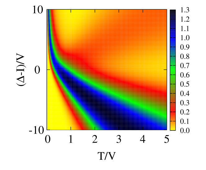
Figure 1: (online colour at www.ann-phys.org) Specific heat $C_{{\mathcal{N}}=2}$ of the two-site infinite-$U$ SIAM cluster with nearest neighbor repulsion $I$ and level splitting $\Delta=\epsilon_{\rm c}-\epsilon_{\rm a}$. The density plot of $C_{{\mathcal{N}}=2}$ visualizes the evolution of the specific heat peak with $\Delta-I$.

4 Summary

Summarizing, we have revisited the Kotliar and Ruckenstein slave boson representation for the $U=\infty$ single impurity Anderson model. It backs on the introduction of three complex slave boson fields, subject to three constraints. The $U(1)\times U(1)\times U(1)$ gauge symmetry of this representation allows to gauge away the phases of all three slave boson fields in the continuum limit. We then implemented a path integral procedure involving radial slave boson fields defined for discrete time steps. The correctness of several Kotliar and Ruckenstein renormalization factors has been verified through the exact evaluation of the partition function and expectation values for a strongly interacting two-site model. In particular, the expectation value of the radial slave boson fields was shown to be finite, and does not refer to the introduction of spurious Bose condensates. On the contrary they directly represent the density of empty or singly occupied sites. Correlation functions and thermodynamics can be correctly captured in this framework. Non-local Coulomb interaction can be taken into account as well, paving the way for calculations in the lattice case. For this purpose suitably modified k-matrices, which enter the partition function Eq. (22), have to be identified.

Acknowledgments.  R.F. is grateful for the warm hospitality at the EKM of Augsburg University where part of this work has been done, and to the Région Basse-Normandie and the Ministère de la Recherche for financial support. This work was supported by the Deutsche Forschungsgemeinschaft through TRR 80 (T.K.). Especially, we would like to thank Ulrich Eckern for his support and encouragement to pursue our work over so many years. It is a great pleasure to dedicate this paper to him on the occasion of his 60th birthday.

References

• [1] A. P. Malozemoff, J. Mannhart, and D. Scalapino, Phys. Today 58, 41 (2005).
• [2] J. G. Bednorz and K. A. Müller, Z. Physik B 64, 189 (1986); B. Raveau, C. Michel, M. Hervieu, and D. Groult, Crystal Chemistry of High-Tc Superconducting Copper Oxides, Springer Series in Material Science 15, Springer-Verlag Berlin, Heidelberg, New York (1991).
• [3] R. von Helmolt, J. Wecker, B. Holzapfel, L. Schultz, and K. Samwer, Phys. Rev. Lett. 71, 2331 (1993); Y. Tomioka, A. Asamitsu, Y. Moritomo, H. Kuwahara, and Y. Tokura, Phys. Rev. Lett. 74, 5108 (1995); B. Raveau, A. Maignan, and V. Caignaert, J. Solid State Chem. 117, 424 (1995); A. Maignan, C. Simon, V. Caignaert, and B. Raveau, Solid State Commun. 96, 623 (1995).
• [4] H. Kawazoe, H. Yasakuwa, H. Hyodo, M. Kurota, H. Yanagi, and H. Hosono, Nature 389, 939 (1997).
• [5] L. Li, C. Richter, S. Paetel, T. Kopp, J. Mannhart, and R.C. Ashoori, Science 332, 825 (2011).
• [6] H. Ohta et al, Nature Mat. 6, 129 (2007); R. Frésard, S. Hébert, A. Maignan, L. Pi, and J. Hejtmanek, Phys. Lett. A 303, 223 (2002); A. Maignan, C. Martin, R. Frésard, V. Eyert, E. Guilmeau, S. Hébert, M. Poienar, and D. Pelloquin, Solid State Commun. 149, 962 (2009).
• [7] N. Reyren, S. Thiel, A. D. Caviglia, L. Fitting Kourkoutis, G. Hammerl, C. Richter, C. W. Schneider, T. Kopp, A.-S. Rüetschi, D. Jaccard, M. Gabay, D. A. Muller, J.-M. Triscone, and J. Mannhart, Science 317, 1196 (2007).
• [8] V. Eyert, U. Schwingenschlögl, C. Hackenberger, T. Kopp, R. Frésard, and U. Eckern, Prog. Solid State Chem. 36, 156 (2008).
• [9] U. Lüders, W. C. Sheets, A. David, W. Prellier, and R. Frésard, Phys. Rev. B 80, 241102(R) (2009).
• [10] A. Perelomov, Commun. Math. Phys. 26, 222 (1972).
• [11] E. Tüngler and T. Kopp, Nucl. Phys. B 443, 516 (1995).
• [12] S. E. Barnes, J. Phys. F 6, 1375 (1976); ibid. 7, 2637 (1977).
• [13] P. Coleman, Phys. Rev. B 29, 3035 (1984).
• [14] G. Kotliar and A. E. Ruckenstein, Phys. Rev. Lett. 57, 1362 (1986).
• [15] T. Kopp, F.J. Seco, S. Schiller, P. Wölfle, Phys. Rev. B 38, 11835 (1988).
• [16] T. C. Li, P. Wölfle, and P. J. Hirschfeld, Phys. Rev. B 40, 6817 (1989).
• [17] R. Frésard and P. Wölfle, Int. J. of Mod. Phys. B 6, 685 (1992); ibid. 6, 3087 (1992).
• [18] R. Frésard and G. Kotliar, Phys. Rev. B 56, 12 909 (1997).
• [19] N. Pavlenko and T. Kopp, Phys. Rev. B. 72, 174516 (2005).
• [20] F. Lechermann, A. Georges, G. Kotliar, and O. Parcollet, Phys. Rev. B 76, 155102 (2007).
• [21] R. Frésard and T. Kopp, Phys. Rev. B. 78, 073108 (2008).
• [22] R. Frésard, J. Kroha, and P. Wölfle, Theoretical Methods for Strongly Correlated Systems, A. Avella and F. Mancini (eds.), Springer Series in Solid-State Sciences 171, 65-101, DOI 10.1007/978-3-642-21831-6_3, Springer-Verlag Berlin Heidelberg (2012).
• [23] J. Kroha, P.J. Hirschfeld, K.A. Muttalib, and P. Wölfle, Solid State Commun. 83, 1003 (1992); J. Kroha, P. Wölfle, and T.A. Costi, Phys. Rev. Lett. 79, 261 (1997); J. Kroha and P. Wölfle, Acta Phys. Pol. B 29, 3781 (1998); S. Kirchner and J. Kroha, J. Low Temp. Phys. 126, 1233 (2002).
• [24] N. Read, D. M. Newns, J. Phys. C 16, L1055 (1983); ibid. 3273 (1983); D. M. Newns and N. Read, Adv. in Physics 36, 799 (1987).
• [25] R. Frésard and T. Kopp, Nucl. Phys. B 594, 769 (2001).
• [26] R. Frésard, H. Ouerdane, and T. Kopp, Nucl. Phys. B 785, 286 (2007).
• [27] S. Florens, A. Georges, G. Kotliar, and O. Parcollet, Phys. Rev. B 66, 205102 (2002).
• [28] W. Metzner and D. Vollhardt, Phys. Rev. Lett. 62, 324 (1989); W. Metzner, Z. Phys. B 77 253 (1989); W. Metzner and D. Vollhardt, Phys. Rev. B 37, 7382 (1988).
• [29] L. Lilly, A. Muramatsu, and W. Hanke, Phys. Rev. Lett. 65, 1379 (1990); R. Frésard, M. Dzierzawa, and P. Wölfle, Europhys. Lett. 15, 325 (1991).
• [30] R. Frésard and P. Wölfle, J. Phys.: Condens. Matter 4, 3625 (1992); B. Möller, K. Doll, and R. Frésard, J. Phys.: Condens. Matter 5 4847 (1993); G. Seibold, E. Sigmund, and V. Hizhnyakov, Phys. Rev. B 57, 6937 (1998); G. Seibold, Phys. Rev. B 58, 15520 (1998); G. Kotliar, E. Lange, and M. J. Rozenberg, Phys. Rev. Lett. 84, 5180 (2000); R. Frésard and M. Lamboley, J. Low Temp. Phys. 126, 1091 (2002); Q. Yuan and T. Kopp, Phys. Rev. B 65, 085102 (2002); P. Korbel, W. Wojcik, A. Klejnberg, J. Spałek, M. Acquarone, and M. Lavagna, Eur. Phys. J. B 32, 315 (2003); L. F. Feiner and A. M. Oleś, Phys. Rev. B 71, 144422 (2005); M. Raczkowski, R. Frésard, and A. M. Oleś, Phys. Rev. B 73, 174525 (2006); M. Raczkowski, R. Frésard, and A. M. Oleś, Europhys. Lett. 76, 128 (2006); J. Lorenzana and G. Seibold, Low Temp. Phys. 32, 320 (2006); N. Pavlenko and T. Kopp, Phys. Rev. Lett. 97, 187001 (2006); A. Rüegg, S. Pilgram, and M. Sigrist, Phys. Rev. B 75, 195117 (2007); F. Lechermann, Phys. Rev. Lett. 102, 046403 (2009); A. Isidori and M. Capone, Phys. Rev. B 80, 115120 (2009).
• [31] In Eq. (31) we discarded the remaining $4\times 4$ block that vanishes.
• [32] R. Frésard, H. Ouerdane, and T. Kopp, EPL 82, 31001 (2008).
• [33] W.F. Brinkman and T.M. Rice, Phys. Rev. B 2, 4302 (1970).
• [34] W. Zimmermann, R. Frésard, and P. Wölfle, Phys. Rev. B 56, 10 097 (1997).