Geometrical defects in two-dimensional melting of many-particle Yukawa systems

Abstract

We perform Langevin dynamics simulations and use polygon construction method to investigate two-dimensional (2D) melting and freezing transitions in many-particle Yukawa systems. 2D melting transitions can be characterized as proliferation of geometrical defects — non-triangular polygons, obtained by removing unusually long bonds in the triangulation of particle positions. A 2D liquid is characterized by the temperature-independent number of quadrilaterals and linearly increasing number of pentagons. We analyse specific types of vertices, classified by the type and distribution of polygons surrounding them, and determine temperature dependencies of their concentrations. Critical points in a solid-liquid transition are followed by the peaks in the abundances of certain types of vertices.

I Introduction

For a few decades melting and freezing transitions in two-dimensional many-particle systems have been investigated in a variety of experimental and computational studies, without reaching a definite conclusion regarding its nature. According to the most widely accepted Kosterlitz-Thouless-Halperin-Nelson-Young (KTHNY) theory, melting of a single two-dimensional (2D) crystal occurs via two continuous phase transitions, first from a solid to hexatic phase, and then from the hexatic to an isotropic fluid Nelson ; Young . The theory also predicts, what it is proliferation of unbound topological defects — dislocations and then free disclinations — what plays a crucial role in 2D phase transitions and breaks positional and orientational order. Some experiments and theoretical studies, however, suggest a first-order grain-boundary-induced melting scenario in polycrystalline systems Nosenko ; Chui .

Although in 2D a true crystalline order can not survive at finite temperatures $kT>0$ Mermin ; Hohenberg , a quasi-long range translational order is observed at the conditions of strong coupling, for example, in complex plasma layers Knapek or charged colloidal suspensions Murray . Over the years a broad range of empirical criteria was developed to accurately determine melting and crystallization points Wang . Perhaps one of the most famous examples is the Lindemann criterion, which has been applied extensively in three-dimensional melting and freezing, while its generalized version has been used in some studies of two-dimensional transitions Bedanov . Other methods frequently make use of topological defect fractions, bond orientational order parameters, orientational and positional correlation functions as well as Einstein frequencies Hartman1 . In a recent work, a polygon construction method by Glaser and Clark Glaser1 ; Glaser2 ; Lansac was employed to characterize transitions in a rapidly heated and cooled two-dimensional complex plasma experiment Suranga .

Systems of strongly correlated particles in complex plasmas are of particularly high importance in the experimental studies of phase transitions. Complex plasma usually consists of polymer microparticles immersed in a weakly ionized gas, where distinct dust grains are known to interact through the Yukawa (Debye-Hückel) interaction Konopka . Convenient time and length scales of these systems allow for the direct optical observation of collective many-particle phenomena as well as accurate measurements of individual particle positions by the means of video microscopy Morfill ; Chu ; Thomas0 .

In a recent experiment, the phenomenon of superheating was observed in a solid state of two-dimensional complex plasma Feng . It was demonstrated, that during a rapid heating process, the concentration of defects can stay low and complex plasma can retain the properties of a solid even at the temperatures above a melting point. The same experimental results were later analysed by the method of geometrical defects Suranga , originally developed by Glaser and Clark, which we use in the current work.

Geometrical defects in a polygon construction method are identified by removing unusually long bonds in the triangulation map of particle positions, so that resulting polygons have three or more sides. It was shown, that this method provides great sensitivity and unveils some interesting features, undetectable by the conventional analysis of topological defects Suranga . As another measure of disorder, the abundance of different kinds of vertices, grouped according to the type and order of the adjacent polygons, was suggested in the same work.

In the present contribution we report numerical studies of two-dimensional melting and crystallization in strongly coupled Yukawa systems. Langevin dynamics simulations are performed to simulate gradual heating and cooling. Critical points are determined employing orientational order parameters and topological defect fractions. However, the main motivation behind the current work is to present the method of geometrical defects and vertex fractions in the polygon construction as a sensitive tool to analyse the order-disorder transitions and characterize the state of a 2D system. Furthermore, our findings resolve the issue of the prominent peaks in the temperature-dependencies of certain types of vertex concentrations Suranga , by showing, that peaks correspond to the critical points in the initial and final stages of the order-disorder phase transition.

In the following section we briefly describe the model system and simulation methods, as well as essential tools used in the analysis of phase transitions. Main results of the simulations and numerical analysis are presented in Section III, while Section IV summarizes the article.

II Simulation

II.1 Model system

A widely used approximation to describe interactions between particles in complex plasmas is the Yukawa inter-particle potential Konopka

$$V_{ij}=Q^{2}(4\pi\varepsilon_{0}r_{ij})^{-1}\exp(-r_{ij}/\lambda_{\rm D}).$$ (1)

Here $Q$ is the charge of a particle, $r_{ij}$ is the distance between particles $i$ and $j$, $\lambda_{\rm D}$ stands for the Debye length, which accounts for the screening of the interaction by other plasma species.

Strongly coupled many-particle systems with Yukawa interactions are fully characterized by two dimensionless parameters, namely the coupling strength $\Gamma=Q^{2}/(4\pi\varepsilon_{0}bk_{\rm B}T)$ and screening parameter $\kappa=b/\lambda_{\rm D}$, where $b$ is the two-dimensional Wigner-Seitz radius Kalman . In the simulations presented here we set the screening strength to the constant value of $\kappa=2$.

As a scale of length in our numerical simulations it is convenient to choose the Wigner-Seitz radius $b$, which is directly related to the areal number concentration of particles, $n=1/(\pi b^{2})$. Therefore, the corresponding scale of energy is $\epsilon=Q^{2}/(4\pi\varepsilon_{0}b)$ and time is scaled according to the value of an inverse plasma frequency

$$\omega_{0}^{-1}=\left(\frac{Q^{2}}{4\pi\varepsilon_{0}mb^{3}}\right)^{-1/2}.$$ (2)

The model system consists of $N=2430$ identical particles in a 2D rectangular box of area $85.71\times 89.07$, interacting via the Yukawa potential. Periodic boundary conditions are applied and, since the inter-particle potential is short-ranged, the cut-off distance is set to $r_{\rm c}=8$. Only particle pairs separated by less than $r_{\rm c}$ are taken into account in the force calculation.

We study order-disorder transitions in the model system by performing Langevin dynamics simulations with slow changes of temperature. Particle positions are updated according to the dimensionless Langevin equation

$$\mathbf{\ddot{r}}_{i}=-\nabla_{i}V(\mathbf{r}_{1},\dotsc,\mathbf{r}_{N})-\mu\mathbf{\dot{r}}_{i}+\mathbf{f}_{i},$$ (3)

where $\mathbf{f}_{i}$ represents a randomly fluctuating Brownian force. In a thermodynamic equilibrium $\left<\mathbf{f}_{i}(t)\right>=0$, while the friction coefficient $\mu$ is related to the Gaussian noise $\mathbf{f}_{i}(t)$ by the fluctuation-dissipation theorem Gunsteren

$$\left<{\rm f}_{i}(t){\rm f}_{j}(t^{\prime})\right>=2\mu kT_{\rm ref}\delta_{ij}\delta(t-t^{\prime}),$$ (4)

where $i,\,j\in\{1,\dotsc,N\}$ and $kT_{\rm ref}$ is the desired target temperature in the units of $\epsilon$. In our simulations we use $\mu=0.2$. The Langevin equation is integrated numerically employing an impulse method of integration Skeel .

II.2 Analysis

A common way of analysing the structure of 2D many-particle systems is calculation of a Delaunay triangulation, which yields a network of bonds connecting each particle with its nearest neighbours. A coordination number can be assigned to each particle, which is a number of the triangulation bonds between the particle and its closest neighbours. The coordination number of a particle in a perfect hexagonal lattice is always equal to six. Topological defects are identified as particles with a different coordination number, usually five or seven.

Two most common defect types are the disclination (a single particle with a non-sixfold coordination) and the dislocation (two connected particles with five and seven closest neighbours) Radzvilavicius . Quite frequently defects organize themselves in lengthy chains or grain boundaries, indicating a polycrystalline structure of the system. As an alternative, a Voronoi construction is sometimes used in the context of 2D dusty plasmas, where defects are identified as non-six-sided polygons Nosenko ; Feng2 ; Thomas ; Feng3 .

To quantify the abundance of topological defects, we use the defect fraction $\rm DF$, which is defined as a number of vertices with a coordination number other than six, normalized to the total number of particles $N$ Feng3 .

The polygon construction is a different way of characterizing defects in 2D systems Glaser1 ; Glaser2 ; Suranga and helps to identify empty volumes in 2D liquids Bernal . The authors of Glaser1 analysed bond-angle and bond-length probability distributions in dense 2D liquids. It was shown, that disordered regions of a liquid exhibit multiple peaks in a bond-angle probability distribution, with extra peaks corresponding to the square lattice. At the same time, triangularly-oriented clusters had a single peak and well expressed triangular order. The structure of a two-dimensional system therefore was described as a square-triangular tiling containing numerous tiling faults.

A triangle, which is the only kind of polygon in the initial triangulation of particle positions, is considered as a non-defective entity. To identify geometrical defects, certain bonds are removed from the triangulation map, so that two polygons sharing a common bond are merged into one. Two possible approaches for the selection of bonds were suggested: either use a bond-length threshold, or identify a bond that is opposite to the unusually large angle between a pair of adjoining bonds. In our analysis we follow the authors of Glaser1 ; Suranga and use the critical bond-angle of $\alpha=75^{\circ}$.

The construction of a polygon map is illustrated in Figure 1. The first panel (a) shows the 2D triangulation map of particle positions, where most of the particles are connected with six closest neighbours. Some vertices, however, have five or seven bonds and are marked by small triangles and squares. These particles are considered as topological defects and are all the part of a lengthy grain boundary. Triangulation bonds marked by bold lines are facing bond-angles larger than the critical value of $\alpha=75^{\circ}$ and therefore are selected for removal. The resultant polygon map is presented in the second panel (b). Geometrical defects are identified as non-triangular polygons, that is, quadrilaterals and pentagons. Although the defects appear in a close vicinity of the grain boundary, there is no one-to-one correspondence between the polygons and topological defects.

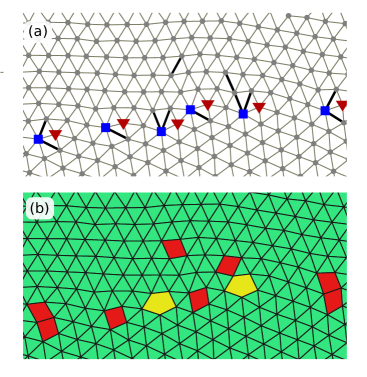
Figure 1: Triangulation map of a polycrystalline 2D Yukawa solid, with topological defects marked as squares and triangles (a). By removing the bonds facing unusually large angles (marked by bold lines), the polygon construction (b) is obtained. In general there is no one-to-one correspondence between topological and geometrical defects.

The polygon construction contains geometrical information about bond lengths and angles, as well as topological information about the nearest-neighbour connections. The method has also the advantage of providing a gradation in the severity of geometrical defects. Quadrilaterals are the least severe, while pentagons and hexagons are more severe and indicate large excess volumes. Topological defects, on the other hand, provide only a binary measure of local orientational disorder, that is, at the specific location of a vertex, there either is a defect, or there is not.

The gradation of defects in the polygon method allows for a greater sensitivity identifying and classifying disorder Suranga . To characterize the state of our model system and the abundance of geometrical defects we use four distinct order parameters $P_{n}=N_{n}/(2N)$ ($n=3,\,4,\,5,\,6$), defined as the number of polygons with $n$ sides $N_{n}$, normalized to the doubled number of particles $2N$.

Figure 2 provides a classification scheme for vertices, according to the configuration of polygons arranged around them. The abundance of different vertex types serves as another way to characterize disorder and identify the manner in which polygons cluster together. In a perfect crystal, one would observe only vertices of type A. In a regular square-triangular tiling, only vertices of types A–D are allowed Glaser1 . Types J and K correspond to the topological disclinations, while a vertex L features a severe pentagonal defect. To quantify the abundance of different vertex types, we calculate fractions $X_{\rm Y}$, defined as the number of vertices of a certain type $\rm Y$ normalized to the total number of particles in the polygon construction.

Unexpected spikes in the time dependencies of parameters $X_{\rm E}$ and $X_{\rm F}$ were detected in the analysis of the recent super-heating experiment Suranga , suggesting that some of the vertices might be metastable or exist only in a narrow range of temperatures. One of the goals of our work is to resolve this issue.

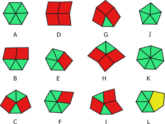
Figure 2: Twelve types of vertices, frequently observed in the polygon construction of 2D Yukawa systems. Vertices are classified by the number and relative distribution of polygons around a vertex.

Phase transitions in two-dimensional systems are usually identified by the sudden change in orientational or translational order parameters. The local orientational order parameter for a particle $j$ is defined as Strandburg

$$\psi_{6j}=\frac{1}{N_{j}}\sum_{k=1}^{N_{j}}{\rm exp}(6i\theta_{jk}),$$ (5)

where $\theta_{jk}$ is the angle between the bond connecting particles $j$ and $k$ and some fixed direction. $N_{j}$ is the coordination number of the particle $j$. The magnitude $\lvert\psi_{6j}\rvert$ is close to unity for a particle inside a hexagonal lattice but is small close to the domain walls (grain boundaries) or in a liquid. On the other hand, the value of a complex argument $\arg(\psi_{6j})$ represents the angular orientation of a neighbourhood or entire domain.

The parameter $\psi_{6}=\lvert\left\langle\psi_{6j}\right\rangle\rvert$, that is, a magnitude of the averaged complex orientational order parameter, defines the overall orientational order of the system. In polycrystalline solids, however, complex numbers $\psi_{6j}$ corresponding to the particles from different domains, tend to cancel in the averaging process. Therefore, $\psi_{6}$ approaches very small values in the limit of an infinite sample size. Another parameter can be used in such cases, namely $\psi_{\lvert 6\rvert}=\left\langle\lvert\psi_{6j}\rvert\right\rangle$, which represents the average local orientational order of the whole system Wang .

III Results

We start our simulations with a defect-free lattice in a strongly-coupled state and the temperature of $kT=10^{-7}$. The system is then slowly heated over the period of time of $\Delta t=240\,000$, until the temperature of $kT=0.005$ is reached. The stage of steady cooling then follows, restoring the temperature to its initial value (see, for example, Figure 8-e). The chosen rate of heating is low enough to reach the equilibrium at each step of the simulation outside the region of a fast order-disorder transition. Therefore, lower rates of heating and cooling would not substantially change the qualitative results of our numerical experiments, except in the close vicinity of the transition, which we discuss later.

The peak temperature is chosen to be well above the melting point, as found by the previous studies Hartman1 ; Hartman2 . The actual kinetic temperature of the system is calculated from observed particle velocities, $kT=\langle v_{i}^{2}\rangle/2$ and is found to fluctuate around the prescribed values of $kT_{\rm ref}$, with the fluctuations being proportional to the temperature. We keep track of the order parameters and defect fractions throughout the whole cycle. In this section we first investigate the orientational order of the 2D system, and then turn to the defects and polygons.

The initial values of both orientational order parameters $\psi_{6}$ and $\psi_{\lvert 6\rvert}$ are very close to unity, as Figure 3 shows, and correspond to the defect-free hexagonal lattice. The system exhibits a sudden loss of orientational order in the temperature range of $kT=0.0025\text{--}0.0027$ (the corresponding coupling parameter values are $\Gamma=370\text{--}400$), which is the signature of a melting phase transition. Our observations are in a fair agreement with Hartman1 ; Hartman2 , where phase transitions in two similar 2D systems were observed near the values of $\Gamma=384$ and $\Gamma=415$. At the end of the heating phase $\psi_{6}$ drops below $0.1$ and $\psi_{\lvert 6\rvert}$ to the value of approximately $0.5$.

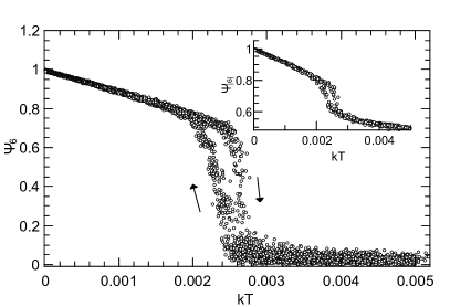
Figure 3: Averaged orientational order parameters $\psi_{6}$ and $\psi_{\lvert 6\rvert}$ of a 2D Yukawa system during the heating and cooling simulation cycle.

As the temperature is gradually lowered, a 2D Yukawa liquid freezes back to the hexagonal lattice. However, the evolution of the order parameters does not follow exactly the same path as in the case of melting and hysteresis is observed (Figure 3). $\psi_{6}$ stays low until the temperature of $kT=0.0024$ is reached, which is lower than the melting point. Changes in $\psi_{\lvert 6\rvert}$ also occur at somewhat lower temperatures and are not as abrupt as in the case of melting. As we show later, the effect of hysteresis is most likely a result of the finite rate of heating and cooling.

The concentration of topological defects during the stage of slow heating exhibits a similar trend, with a weak temperature dependence before and after the transition, see Figure 4. A sudden proliferation of defects is observed in the range of $kT\approx 0.0025\text{--}0.0027$. Changes in the defect concentration during the gradual cooling are not as abrupt and occur at somewhat lower temperatures, $kT\approx 0.0024\text{--}0.0022$.

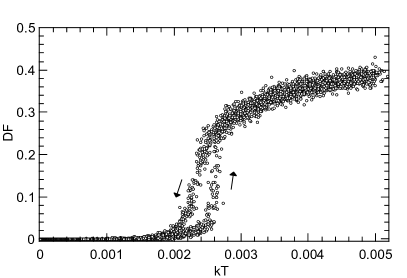
Figure 4: Topological defect fraction $\rm DF$ as a function of the kinetic temperature $kT$.

Four typical snapshots of particle positions during the transition are shown in Figure 5. Here triangles correspond to the particles with only five nearest neighbours, while squares mark positions of vertices with seven triangulation bonds. In a solid phase (Figure 5-a), defects mostly appear as quartets, composed of two disclinations with five bonds and two vertices with seven neighbours. Alternatively, this four-defect complex can be treated as a bound pair of two dislocations. Apparently, this kind of topological fault does not significantly change either positional or orientational order. Larger defect complexes, consisting of more than four defective vertices emerge before the melting transition.

As it is illustrated in the second panel of the figure, during the melting transition (e.g. $kT=0.0026$) defect complexes grow and spread. However, as it can be seen in Figure 5-b, large defect-free patches still exist, suggesting, that the transition from a defect-free lattice to the disordered state is not homogeneous. Bound dislocations are still found in the ordered patches, however are seldom seen. While some disclinations and dislocations are present, they are clearly not the main cause of the loss of order; most of these defects appear as parts of larger regions of condensed defect groups and chains. This observation supports the theory of grain-boundary induced melting Nosenko ; Chui ; Quinn , or possibly the coexistence of hexatic and liquid states, as described in Qi . Further investigations of larger systems would be needed to unambiguously determine the mechanism of the melting transition.

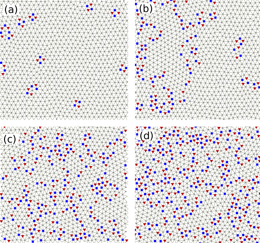
Figure 5: Typical arrangements of topological defects during the melting transition of a 2D Yukawa system. Triangles here represent particles with five closest neighbours, while squares mark vertices with the coordination number equal to seven. The corresponding temperatures are $kT=0.00245$ (a), $0.0026$ (b), $0.0027$ (c) and $0.0045$ (d).

Finally, at the end of the transition — Figure 5-c — topological defects form large inter-connected complexes, destroying orientational order completely. Free dislocations and disclinations can still be occasionally found in the larger groups of defects. The distribution of defects becomes homogeneous in a high-temperature liquid (Figure 5-d).

As the system is slowly cooled, defect complexes and large defect-free regions can still be found at the temperatures as low as $kT=0.0022$, together with some free dislocations. At lower temperatures, however, these complexes tend to shrink and rearrange, eventually leaving only bound and free dislocations as well as interstitial particles. The final configuration corresponds to the nearly perfect triangular lattice with a few free dislocations, leading to the low defect concentration and values of the orientational order parameter close to unity.

Previous studies of similar systems Schweigert suggest that the effect of hysteresis might be caused by the finite rate of heating and cooling. We test this hypothesis by analysing the evolution of topological defect fraction at the constant prescribed temperature of $kT_{\rm ref}=0.00243$, starting from either liquid or solid initial state. According to Figure 6, at this temperature the system slowly switches between high and low values of the order parameter, corresponding to the defect configurations depicted in parts (a) and (c) of Figure 5. Therefore, there is a range of temperatures, in which ordered and disordered states are unstable and have approximately the same probabilities to be observed, as reported in Schweigert ; Morf , and no hysteresis should occur in the limit of infinite simulation time.

Figure 6: Time series for the topological defect fraction $\rm DF$ at the prescribed temperature of $kT_{\rm ref}=0.00243$.

Let us now turn to the analysis of the polygon construction. The initial defect-free lattice corresponds to a triangular tiling. Therefore, the triangle is the only type of polygon present in the original configuration. As the system is continuously heated, quadrilaterals and occasional pentagons appear. As it can be seen in Figure 7, quadrilateral defects tend to cluster together, forming long chains or “ladders” in a solid phase (a) or larger patches of a distorted square lattice in a liquid (c). Defect-free zones are still present during the initial stage of solid-liquid transition, e.g. at the temperature of $kT=0.0026$ as depicted in Figure 7-b. Solitary hexagons appear much later and are most abundant in the high-temperature Yukawa liquid (d).

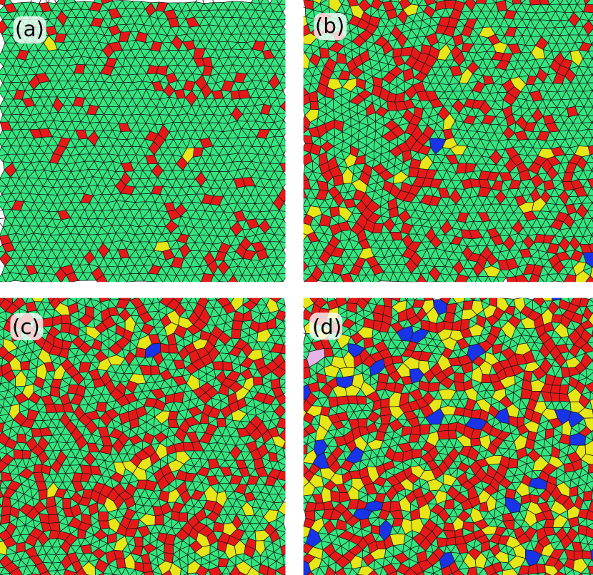
Figure 7: Typical arrangements of geometrical defects during the gradual heating stage in a 2D Yukawa system: solid phase at $t=45\,002$ (a), configurations during (b) and right after (c) the solid-liquid transition and high-temperature liquid phase at $t=120\,000$ (d). The corresponding temperatures are $kT=0.0018$ (a), $0.0026$ (b), $0.0027$ (c) and $0.0045$ (d).

The quadrilateral is a first type of geometrical defect to appear in a low-temperature solid, first seen near the temperature of $kT=5\cdot 10^{-4}$. This is as expected, since the quadrilateral is the least severe geometrical defect. Also it is the most abundant type of defect in both solid and liquid states. The parameter $P_{4}$, defined as a number of quadrilateral defects normalized to $2N$, increases steadily as the temperature rises during early stages of heating. As it is demonstrated in the second panel of Figure 8, the proliferation rate gets significantly higher as the temperature reaches the value of $kT=0.0025$ and the melting transition begins. The rapid transition ends at around $kT=0.0027$, where the order parameter fluctuates around the value of $P_{4}=0.20$.

The abundance of quadrilateral defects in the two-dimensional Yukawa liquid does not change significantly as the temperature is further increased. Therefore, we suggest, that a 2D liquid right after the phase transition can be characterized by the temperature-independent value of the quadrilateral order parameter close to $P_{4}=0.20\pm 0.01$. These observations are illustrated in Figure 8 as time series for the order parameter (b) and temperature $kT$ (e).

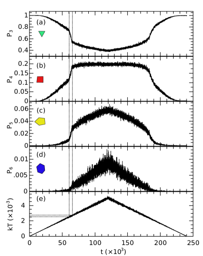
Figure 8: Time series for order parameters $P_{3}$ (a), $P_{4}$ (b), $P_{5}$ (c) and $P_{6}$ (d), characterizing the abundances of triangles, quadrilaterals, pentagons and hexagons in the polygon construction of the 2D Yukawa system. Time series of the kinetic temperature $kT$ is presented in the last panel (e). Two vertical lines mark the beginning and ending points of the melting transition.

Occasional pentagonal defects are first spotted at the temperature of nearly $kT=0.001$. The most significant proliferation of these defects takes place in the range of $kT=0.0025\text{--}0.0027$, where the value of a pentagonal order parameter changes from $P_{5}=0.01$ to $P_{5}=0.03$. After the melting transition, $P_{5}$ increases almost linearly with the temperature, at a constant rate. We may conclude, that in the context of pentagonal defects, the liquid state can be characterized by values of the order parameter $P_{5}>0.03$ and a steady growth in a number of pentagons.

In our simulations we observe only a relatively small number of hexagonal defects, with the highest value of an order parameter close to $P_{6}\approx 0.012$. Although the time and temperature dependencies of $P_{6}$ are rather noisy (see Figure 8-d), some general observations can still be made. The most noticeable spread of hexagons starts at about $kT=0.0025$, which roughly coincides with the start of the melting transition. Afterwards, $P_{6}$ seems to increase steadily.

Geometrical defects arrange themselves around the particles in a variety of ways. Some of the most frequent are classified in Figure 2 as vertex types A to L Glaser1 ; Suranga . In a perfect triangular lattice, one would observe only the type A, where six triangles join forming a hexagon. In a liquid, where quadrilaterals tend to form interconnected complexes and “ladders” (Figure 7), the number of vertices B, D, G and H is expected to increase.

As we can see, the arrangement of polygons with respect to a certain vertex can be used as an indicator of disorder throughout melting or freezing transitions. Therefore, we further investigate the evolution of vertex fractions $X_{\rm Y}=N_{\rm Y}/N$, defined as the ratio of a number of vertices for a certain vertex type $N_{\rm Y}$ to the total number of particles $N$.

Vertices E and F are the first to appear when the defect-free system is slowly heated. Just as the quadrilateral defects, these vertices are first observed at the temperature of $kT\approx 5\cdot 10^{-4}$. Both vertex types E and F contain a single quadrilateral and four or five triangles, and are created by removing an inner (E) or outer (F) bond from a vertex type A. Therefore, the abundances of vertices E and F have essentially identical time and temperature dependencies (third panel of Figure 9).

As the temperature rises, the order parameter $X_{\rm E}$ grows until the critical value of $kT\approx 0.0025$ and the fraction of $X_{\rm E}\approx 0.175$ is reached. As a matter of fact, it is approximately the same temperature that marks the start of the rapid melting transition, i.e. the sudden loss of orientational order, the rapid growth in a number of topological defects, squares and pentagons. As geometrical defects proliferate further at higher temperatures, the number of vertices E and F monotonically diminishes.

Vertex types B and C both contain two quadrilaterals and three triangles, but differ in the order they are arranged around a vertex. Two quadrilaterals of a vertex type B share a common edge (Figure 2), while in a vertex C they are separated by a triangle or two. Vertex concentrations $X_{\rm B}$ and $X_{\rm C}$ depart from zero significantly around $kT=0.001$ and grow further with the kinetic temperature. The order parameter $X_{\rm B}$ reaches its highest value of $0.14$ at the temperature of $kT\approx 0.0027$, which coincides with the final transition to the liquid phase (Figure 9). Approximately the same is true for the vertex fraction of the type C, which reaches its highest value $X_{\rm C}\approx 0.12$ close to the temperature of $kT\approx 0.0027$. As the 2D liquid is heated further, the concentrations of vertices B and C decreases.

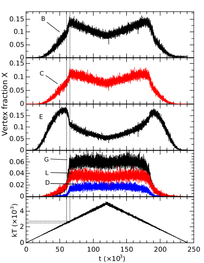
Figure 9: Time series for vertex fractions of vertex types B-L and the temperature $kT$. The time dependence of a vertex fraction $X_{\rm F}$ is virtually identical to the one for vertex E and therefore is not shown here. Vertical lines mark the beginning and ending points of the rapid order-disorder transition.

Vertex fractions for types D, G, H, L and I all share similar time and temperature dependencies (fourth panel of Figure 9). They all feature a steady growth before the temperature of $kT=0.0025$ is reached, rapid change throughout the melting transition and a weak temperature dependence in a liquid state. Right after the transition, that is, temperatures above $kT=0.0027$, the vertex fraction D stays close to a value of $X_{\rm D}=0.017$, while those for other types fluctuate around $X_{\rm G}=0.060$, $X_{\rm H}=0.035$, $X_{\rm I}=0.030$, $X_{\rm L}=0.039$.

A few interesting results were obtained in the recent work Suranga , where the evolution of geometrical defects and vertex fractions in a laser-heated complex plasma was studied. It should be noted, though, that the goal of the study was to investigate solid super-heating and not the temperature dependencies of order parameters. The authors did not have a chance to vary the temperature of a system gradually and a heating source was turned on and off abruptly.

First, quadrilateral and pentagonal order parameters in a liquid state of the experimental system were found to be $P_{4}\approx 0.19$ and $P_{5}\approx 0.05$. These values fully agree with and support the results of our simulations. Secondly, the authors of Suranga observed sudden spikes in the abundances of vertex types F and E at the times when the heating source was abruptly turned on and off. Whether it is a signature of vertex metastability or a specific temperature dependence remained unclear. In the view of our simulation results and, specifically Figure 9, we conclude that the reason behind the spikes is an intrinsic temperature dependence of vertex fractions B, C, E and F, with spikes corresponding to the temperatures lower than the final kinetic temperature of a liquid.

Just as in the case of the orientational parameters and topological defect fractions, an evolution of order parameters $P$ and vertex fractions $X$ during the slow crystallization does not exactly duplicate the behaviour throughout the heating phase. For example, a peak in the time dependence of the vertex fraction E corresponds to the temperature of $kT\approx 0.0022$, as opposed to the temperature of $kT\approx 0.0025$ in the case melting. Critical values of $X_{\rm B}$ and $X_{\rm C}$ are also slightly shifted to lower temperatures. In a final configuration after the crystallization, there are seven quadrilateral defects and a corresponding small fraction of vertices B and E (Figure 9).

We have repeated our simulations starting with polycrystalline configurations, obtained from a rapidly cooled 2D Yukawa liquid. The evolution of order parameters throughout the initial heating phase turned out to be slightly configuration-dependent. For example, in a few cases orientational order parameters increased as the polycrystalline solid was heated, while at the same time topological defects diminished. This can be explained by the melting of grain boundaries and simultaneous merging of crystalline domains. Nevertheless, the point of a final transition to the liquid phase was found to be the same as in the case of the hexagonal initial configuration, that is, $kT\approx 0.0027$. Therefore, most of the results presented here would also hold for the melting of a polycrystalline solid.

IV Summary

In this contribution we report the results of Langevin dynamics simulations, performed to investigate two-dimensional melting and crystallization transitions in many particle Yukawa systems, such as those found in complex plasma experiments. To characterize the state of a system, we use a polygon construction method, in which unusually long bonds are deleted from the triangulation map of particle positions. Geometrical defects are identified as non-triangular polygons, while vertices are classified according to the type and order of polygons surrounding them. We also make use of a topological defect fraction and orientational order parameters as conventional tools to analyse phase transitions.

In our simulations of the system with the constant value of screening strength ($\kappa=2$), the solid-to-liquid phase transition takes place in the coupling parameter range of $\Gamma\approx 400\text{--}370$, where rapid changes in order parameters and defect fractions are detected. The orientational and translational order is destroyed by the non-homogeneous growth of large defect complexes and chains, contrary to the KTHNY theory of two dimensional melting, which predicts the emergence of isolated dislocations and disclinations.

To quantify the disorder, we use polygonal order parameters $P$, that is, the normalized number of geometrical defects of a certain kind. It turns out, that a liquid phase can be characterized by the temperature-independent value of a quadrilateral order parameter of $P_{4}\approx 0.20$. In the context of pentagonal defects, the liquid state is characterized by the value of $P_{5}>0.03$.

Concentrations of vertices containing three or more quadrilaterals (D, G, H and I) show only a weak dependence on the temperature in the liquid state, showing the tendency for quadrilaterals to cluster together. Temperature dependencies of vertex fractions of the types B, C, E and F all feature well expressed peaks at the beginning (E, F) or final stages (B, C) of the solid-liquid transition with a very similar behaviour during the recrystallization.

References

- (1) D. R. Nelson and B. I. Halperin, Phys. Rev. B 19, 2457 (1979)
- (2) A. P. Young, Phys. Rev. B 19, 1855 (1979)
- (3) V. Nosenko, S. K. Zhdanov, A. V. Ivlev, C. A. Knapek, and G. E. Morfill, Phys. Rev. Lett. 103, 015001 (2009)
- (4) S. T. Chui, Phys. Rev. Lett. 48, 933 (1982)
- (5) N. D. Mermin, Phys. Rev. 176, 250 (1968)
- (6) P. C. Hohenberg, Phys. Rev. 158, 383 (1967)
- (7) C. A. Knapek, D. Samsonov, S. Zhdanov, U. Konopka, and G. E. Morfill, Phys. Rev. Lett. 98, 015004 (2007)
- (8) C. A. Murray and D. H. Van Winkle, Phys. Rev. Lett. 58, 1200 (1987)
- (9) Z. Wang, A. M. Alsayed, A. G. Yodh, and Y. Han, J. Chem. Phys. 132, 154501 (2010)
- (10) V. M. Bedanov, G. V. Gadiyak, and Y. E. Lozovik, Phys. Lett. A 109, 289 (1985)
- (11) P. Hartmann, Z. Donkó, P. M. Bakshi, G. J. Kalman, and S. Kyrkos, IEEE Trans. Plasma Sci. 35, 332 (2007)
- (12) M. A. Glaser and N. A. Clark, Phys. Rev. A 41, 4585 (1990)
- (13) M. A. Glaser and N. A. Clark, Adv. Chem. Phys. 83, 543 (1993)
- (14) Y. Lansac, M. A. Glaser, and N. A. Clark, Phys. Rev. E 73, 041501 (2006)
- (15) W. D. Suranga Ruhunusiri, J. Goree, Yan Feng, and Bin Liu, Phys. Rev. E 83, 066402 (2011)
- (16) U. Konopka, G. E. Morfill, and L. Ratke, Phys. Rev. Lett. 84, 891 (2000).
- (17) G. E. Morfill and A. V. Ivlev, Rev. Mod. Phys. 81, 1353 (2009)
- (18) J. H. Chu and Lin I, Phys. Rev. Lett. 72, 4009 (1994)
- (19) H. Thomas, G. E. Morfill, V. Demmel, J. Goree, B. Feuerbacher, and D. Möhlmann, Phys. Rev. Lett. 73, 652 (1994)
- (20) Y. Feng, J. Goree, and B. Liu, Phys. Rev. Lett. 100, 205007 (2008)
- (21) G. J. Kalman, P. Hartmann, Z. Donkó, and M. Rosenberg, Phys. Rev. Lett. 92, 065001 (2004)
- (22) W. F. van Gunsteren and H. J. C. Berendsen, Mol. Phys. 45, 637 (1982)
- (23) R. D. Skeel and J. A. Izaguirre, Mol. Phys. 100, 3885 (2002)
- (24) A. Radzvilavicius, E. Anisimovas, J. Phys.: Condens. Matter 23, 385301 (2011)
- (25) Y. Feng, J. Goree, and B. Liu, Phys. Rev. Lett. 104, 165003 (2010)
- (26) H. M. Thomas and G. E. Morfill, Nature (London) 379, 806 (1996)
- (27) Y. Feng, B. Liu, and J. Goree, Phys. Rev. E 78, 026415 (2008)
- (28) J. D. Bernal, Nature (London) 185, 68 (1960)
- (29) K. J. Strandburg, Rev. Mod. Phys. 60, 161 (1988)
- (30) P. Hartmann, G. J. Kalman, Z. Donkó, and K. Kutasi, Phys. Rev. E 72, 026409 (2005)
- (31) I. V. Schweigert, V. A. Schweigert, and F. M. Peeters, Phys. Rev. B 60, 14665 (1999).
- (32) R.H. Morf, Phys. Rev. Lett. 43, 931 (1979).
- (33) R. A. Quinn and J. Goree, Phys. Rev. E. 64, 051404 (2001).
- (34) W. K. Qi, S. M. Qin, X. Y. Zhao, and Y. Chen, J. Phys.: Condens. Matter 20, 245102 (2008)