Entangling homogeneously broadened matter qubits in the weak-coupling cavity-QED regime

Abstract

In distributed quantum information processing, flying photons entangle matter qubits confined in cavities. However, when a matter qubit is homogeneously broadened, the strong-coupling regime of cavity QED is typically required, which is hard to realize in actual experimental setups. Here, we show that a high-fidelity entanglement operation is possible even in the weak-coupling regime in which dampings (dephasing, spontaneous emission, and cavity leakage) overwhelm the coherent coupling between a qubit and the cavity. Our proposal enables distributed quantum information processing to be performed using much less demanding technology than previously.

Distributed architecture is a promising approach for realizing scalable quantum computation Cirac et al. (1999); Barrett and Kok (2005); Lim et al. (2005); Browne et al. (2003); Bose et al. (1999); Feng et al. (2003). Elementary nodes composed of a few qubits are networked to achieve scalable quantum computation. The node separation can potentially suppress decoherence induced by uncontrollable interactions between qubits. Moreover, since the nodes are spatially separated, individual qubits can be easily addressed by the optical field.

A critical operation for realizing distributed quantum computation is the entanglement operation (EO) Cirac et al. (1999); Barrett and Kok (2005); Lim et al. (2005); Browne et al. (2003); Bose et al. (1999); Feng et al. (2003); Ladd et al. (2006); Van Loock et al. (2006); Azuma et al. (2009). To construct an entire network, qubits in distant nodes have to be coupled by EOs. Most EOs are based on photon interference, and the successful execution of an EO can be heralded by detecting a photon at the target port. This approach has been experimentally demonstrated using an ion trap system Moehring et al. (2007). If the EO fails, the two qubits involved should be initialized, which risks destroying the entanglement of other qubits generated by previous EOs. Although EOs typically have such probabilistic properties, previous studies have revealed that only polynomial steps are required to construct large entangled states Barrett and Kok (2005); Nielsen (2004); Duan and Raussendorf (2005); Gross et al. (2006); Matsuzaki et al. (2010), such as a cluster state Raussendorf and Briegel (2001). Moreover, by introducing a quantum memory to each node, EOs can be repeatedly performed until they are successful without destroying prior entanglement Benjamin et al. (2006).

EOs involve optical excitations of matter qubits. However, the excited states are inherently noisy and significantly degrade the target entanglement. For example, nitrogen vacancy (NV) centers in diamond have promising properties such as a long coherence time at room temperature and optical addressability. Entanglement between an NV center and an emitted photon has been demonstrated at a low temperature of about 7 K Togan et al. (2010). However, at room temperature, this otherwise attractive system suffers from strong environmental dephasing originating from interactions with phonons when the system is optically excited. Consequently, it acquires a large homogeneous broadening of the order of THz Fu et al. (2009). Therefore, in such an approach, NV centers can be used for distributed quantum computation only at low temperatures.

One way to overcome homogeneous broadening is to employ high-Q cavities. Previous theoretical proposals of EOs require strong coupling between a matter qubit and the cavity when the matter qubit has large homogeneous broadening Childress et al. (2005); Matsuzaki et al. (2011a, b). However, despite rapid advances in cavity fabrication technology, it is still very difficult to experimentally generate strong coupling between a matter qubit and a high-Q cavity. To realize distributed quantum computation, it is thus essential to examine the possibility of performing an EO in the weak-coupling regime of cavity QED, where damping parameters such as the pure dephasing rate, the spontaneous emission rate, and the cavity decay rate overwhelm the coherent coupling between the cavity and the qubit.

Here, we report that high-fidelity entanglement can be generated between homogeneously broadened matter qubits even in the weak-coupling regime of cavity QED. Remarkably, both spontaneous emission of the qubit and detuning between the photon and the qubit suppress environmental noise even for low-Q cavities, and enable distributed quantum computation to be performed using much less demanding technology than previously. Moreover, since appropriate use of detuning has the potential to overcome the huge homogeneous broadening that is the main obstacle in using NV centers at high temperatures, our analysis provides the possibility of using NV centers for EOs at much higher temperatures than those of current experiments Togan et al. (2010); Sipahigil et al. (2011).

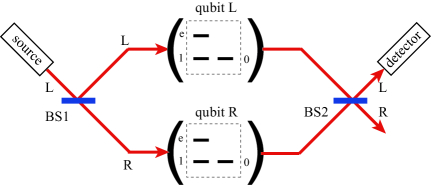
Figure 1: Schematic view of the optical circuit. A single photon is split by a beam splitter (BS1) and is sent to cavities that confine matter qubits with an L-type structure. After interacting with the matter qubits, the photon is combined by another beam splitter (BS2). When the photon reaches the target port and the detector clicks, entanglement is generated between the remote matter qubits.

An outline of the proposed scheme is as follows. The matter qubit is the two ground states ($|0\rangle$ and $|1\rangle$) of an L-type three-level system confined in a two-sided cavity. $|0\rangle$ is optically inactive, whereas $|1\rangle$ is radiatively coupled to an excited state $|e\rangle$ that is subject to level fluctuations due to environmental noise. Two such qubits in cavities are placed symmetrically in a Mach–Zehnder interferometer (Fig. 1). Initially, both qubits are prepared in $(|0\rangle+|1\rangle)/\sqrt{2}$ and a single photon tuned to the cavity frequency is input from the left port of the first beam splitter (BS1). The state vector of the system is given by

$$a_{L}^{{\dagger}}(|00\rangle+|01\rangle+|10\rangle+|11\rangle)/2,$$ (1)

where $|mn\rangle=|m\rangle_{L}|n\rangle_{R}$ denotes the two-qubit state vector and $a_{L}^{{\dagger}}$ ($a_{R}^{{\dagger}}$) creates a photon in the left (right) path. The beam splitters divide a photon as $a_{L}^{{\dagger}}\to(a_{R}^{{\dagger}}+ia_{L}^{{\dagger}})/\sqrt{2}$ and $a_{R}^{{\dagger}}\to(a_{L}^{{\dagger}}+ia_{R}^{{\dagger}})/\sqrt{2}$. For the interaction between the photon and the qubit, when the qubit is in $|0\rangle$ (empty cavity), the input photon is perfectly transmitted through the cavity due to resonance tunneling. In contrast, when the qubit is in $|1\rangle$, the matter qubit modifies the transmitted photon. For example, as we show later, the matter qubit may completely prevent transmission of the photon under some conditions. Then, the photon–qubit interaction removes the terms $a_{L}^{{\dagger}}|10\rangle$, $a_{L}^{{\dagger}}|11\rangle$, $a_{R}^{{\dagger}}|01\rangle$ and $a_{R}^{{\dagger}}|11\rangle$. In other words, the qubit state $|1\rangle$ acts as a “bomb” in the interaction-free measurement Elitzur and Vaidman (1993) in this case. After the photon passes through the second beam splitter (BS2), the state vector is given by

$$-\frac{1}{\sqrt{8}}a_{L}^{{\dagger}}|\phi_{t}\rangle+\frac{i}{2}a_{R}^{{\dagger}}|00\rangle+\frac{i}{\sqrt{8}}a_{R}^{{\dagger}}|\phi_{1}\rangle,$$ (2)

where $|\phi_{t}\rangle=(|01\rangle-|10\rangle)/\sqrt{2}$ and $|\phi_{1}\rangle=(|01\rangle+|10\rangle)/\sqrt{2}$. A photodetector is set to count the photons that exit from the left port of BS2. The detector clicks with a maximum success probability of $1/8$, and the two qubits are then projected onto the target entangled state, $|\phi_{t}\rangle$.

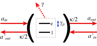
Figure 2: Schematic view of the cavity QED system that we adopted. It consists of a matter qubit and a cavity. The incoming (outgoing) photon fields are denoted by $\hat{a}_{in}$ and $\hat{a}^{\prime}_{in}$ ($\hat{a}_{out}$ and $\hat{a}^{\prime}_{out}$). Three types of damping are considered: environmental pure dephasing ($\gamma_{p}$), spontaneous emission ($\gamma$), and cavity photon leakage ($\kappa$).

We investigate the interaction between the photon and the qubit in a more quantitative manner. Although the master equation has been used in previous analyses Matsuzaki et al. (2011a, b), it is valid in principle only when the damping parameters can be regarded as perturbations Hornberger (2006). In contrast, here, we solve the Heisenberg equations of the overall system including the environment in a non-perturbative manner. Consequently, our results are applicable to highly dissipative cases that include the weak-coupling regime. We investigate a cavity QED system in which a two-level matter qubit ($|1\rangle$, $|e\rangle$) is confined in a two-sided cavity (Fig. 2). The photon dynamics for the qubit state $|0\rangle$ is obtained by removing the matter qubit. This system is characterized by the following parameters: the cavity frequency $\omega_{c}$, the qubit transition frequency $\omega_{q}$, the coherent coupling between the cavity and the qubit $g$, the cavity decay rate $\kappa$, the spontaneous emission rate of the qubit to non-cavity modes $\gamma$, and the pure dephasing rate of the qubit $\gamma_{p}$. The complex frequencies of the cavity and the qubit are defined by $\widetilde{\omega}_{c}=\omega_{c}-i\kappa/2$ and $\widetilde{\omega}_{q}=\omega_{q}-i(\gamma/2+\gamma_{p})$. We denote the destruction operators for the cavity photon and qubit by $c$ and $\sigma(=|1\rangle\langle e|)$, respectively. Their Heisenberg equations are given by

$$\frac{dc}{dt} = -i\widetilde{\omega}_{c}c-ig\sigma-i\sqrt{\kappa/2}[a_{in}(t)+a^{\prime}_{in}(t)],$$ (3)

$$\frac{d\sigma}{dt} = -i\widetilde{\omega}_{q}\sigma-igc-i\sqrt{\gamma}d_{in}(t)$$ (4)

$$-i\sqrt{2\gamma_{p}}[e^{\dagger}_{in}(t)\sigma+\sigma e_{in}(t)],$$

where $d_{in}$ and $e_{in}$ denote the noise operators respectively associated with spontaneous emission and pure dephasing, and $a_{in}$ and $a^{\prime}_{in}$ are the incoming photon fields toward the cavity (see Fig. 2). The outgoing field operators are given by

$$a_{out}(t) = -a^{\prime}_{in}(t)+i\sqrt{\kappa/2}c(t),$$ (5)

$$a^{\prime}_{out}(t) = -a_{in}(t)+i\sqrt{\kappa/2}c(t).$$ (6)

We are interested in the transmission of a single input photon. The transmitted photon consists of elastic and inelastic components. Thus, the state vector evolves on transmission as

$$a^{{\dagger}}|1\rangle\to t_{e}a^{{\dagger}}|1\rangle+t_{i}a^{{\dagger}}e^{{\dagger}}|1\rangle,$$ (7)

where $e^{{\dagger}}$ denotes an environmental excitation near the qubit. As we show in Appendix B1, the fidelity and success probability of our EO are maximized when the spectral width of the input photon is much narrower than the cavity linewidth (i.e., the long pulse limit). We thus assume the long pulse limit in the remainder of the paper. The coefficients $t_{e}$ and $t_{i}$ are then determined by considering the linear response to a classical continuous wave. Setting $a_{in}=Ee^{-i\omega_{c}t}$ and $a^{\prime}_{in}=d_{in}=e_{in}=0$, the dimensionless system variables ($x_{c}=i\sqrt{\kappa/2}\ \langle c\rangle/a_{in}$, $x_{\sigma}=-\sqrt{\kappa/2}\ \langle\sigma\rangle/a_{in}$, and $x_{c^{{\dagger}}c}=\kappa\langle c^{{\dagger}}c\rangle/2|a_{in}|^{2}$) are given by

$$x_{c} = \frac{\kappa(\gamma/2+\gamma_{p}+i\Delta)}{\kappa(\gamma/2+\gamma_{p}+i\Delta)+2g^{2}},$$ (8)

$$x_{\sigma} = \frac{\kappa g}{\kappa(\gamma/2+\gamma_{p}+i\Delta)+2g^{2}},$$ (9)

$$x_{c^{{\dagger}}c} = \kappa\frac{[\gamma+2g^{2}{\rm Re}(1/\xi)]{\rm Re}(x_{c})-g\gamma{\rm Re}(x_{\sigma}/\xi)}{\kappa\gamma+2g^{2}(\kappa+\gamma){\rm Re}(1/\xi)},$$ (10)

where $\Delta=\omega_{q}-\omega_{c}$ is the detuning between the qubit and the input photon and $\xi=(\kappa+\gamma)/2+\gamma_{p}+i\Delta$. $t_{e}$ and $t_{i}$ are related to the amplitude and flux transmissivities by $t_{e}=\langle a_{out}\rangle/a_{in}$ and $|t_{e}|^{2}+|t_{i}|^{2}=\langle a_{out}^{{\dagger}}a_{out}\rangle/|a_{in}|^{2}$. Thus, we have

$$t_{e} = x_{c},$$ (11)

$$|t_{i}|^{2} = x_{c^{{\dagger}}c}-|x_{c}|^{2}.$$ (12)

We can confirm that inelastic transmission originates from pure dephasing, since $t_{i}=0$ when $\gamma_{p}=0$. The photon dynamics for the qubit state $|0\rangle$ is obtained by taking the $g\to 0$ limit, where we can confirm that $t_{e}=1$ and $t_{i}=0$. Therefore, the counterpart of Eq. (7) is

$$a^{{\dagger}}|0\rangle\to a^{{\dagger}}|0\rangle.$$ (13)

Using these rigorous photon–qubit interactions [Eqs. (7) and (13)], we reconsider the time evolution of the initial state vector [Eq. (1)]. Since environmental excitation inhibits photon interference at BS2, the state vector that clicks the detector is given by

$$|\psi\rangle=a_{L}^{\dagger}\left(\frac{t_{e}-1}{\sqrt{8}}|\phi_{t}\rangle+\frac{t_{i}}{\sqrt{8}}e_{R}^{\dagger}|\phi_{2}\rangle-\frac{t_{i}}{\sqrt{8}}e_{L}^{\dagger}|\phi_{3}\rangle\right),$$ (14)

where $|\phi_{2}\rangle=(|01\rangle+|11\rangle)/\sqrt{2}$ and $|\phi_{3}\rangle=(|10\rangle+|11\rangle)/\sqrt{2}$. The click probability ${\cal P}$, reduced density matrix $\hat{\rho}$, and fidelity ${\cal F}$ are respectively defined by ${\cal P}=\langle\psi|\psi\rangle$, $\hat{\rho}={\rm Tr}_{a,b}\{|\psi\rangle\langle\psi|\}/\langle\psi|\psi\rangle$, and ${\cal F}=\langle\phi_{t}|\hat{\rho}|\phi_{t}\rangle$. ${\cal F}$ and ${\cal P}$ are given by

$${\cal F} = \frac{|1-t_{e}|^{2}+|t_{i}|^{2}/2}{|1-t_{e}|^{2}+2|t_{i}|^{2}},$$ (15)

$${\cal P} = |1-t_{e}|^{2}/8+|t_{i}|^{2}/4.$$ (16)

We first examine the effects of homogeneous broadening by assuming that both detuning and spontaneous emission are absent ($\Delta=\gamma=0$). In this case, the transmission probability through the cavity is given by $|t_{e}|^{2}+|t_{i}|^{2}=\kappa\gamma_{p}/(\kappa\gamma_{p}+2g^{2})$. Therefore, when $\kappa\gamma_{p}/g^{2}\ll 1$, the cavity nearly completely suppresses transmission of the photon and the present scheme functions with a high fidelity. To achieve ${\cal F}>0.9$ (0.95), $\kappa\gamma_{p}/g^{2}$ should be less than 0.15 (0.07). Consequently, high-Q cavities satisfying $\kappa\gamma_{p}/g^{2}\ll 1$ are required to achieve high-fidelity EOs under a large homogeneous broadening. This is qualitatively consistent with another scheme that employs resonant input photons Childress et al. (2005).

Spontaneous emission usually degrades the figure of merits of quantum devices. In contrast, spontaneous emission makes our protocol more robust against environmental noise and relaxes the cavity conditions, so that a high-fidelity EO becomes possible between homogeneously broadened matter qubits even in the weak-coupling regime ($g<\kappa,\gamma,\gamma_{p}$), as we show in Appendix B2. The origin of infidelity here is inelastic scattering (i.e., entanglement with the environment) that occurs while the matter qubit is being excited. Spontaneous emission reduces the lifetime of the excited state and thus hinders inelastic scattering. However, in actual experiments, it is difficult to artificially increase the spontaneous emission rate and thus this does not provide a practical solution. Therefore, we look for another way to suppress environmental noise using existing technology. We consider the use of detuning.

We briefly explain the physical mechanism of an EO employing a detuned photon. When there is large detuning $\Delta$, Eqs. (8) and (11) give $t_{e}\simeq e^{-i\theta}$, where $\theta=g^{2}/\Delta\kappa$. Namely, when the qubit state is $|1\rangle$, the input photon acquires a phase shift that is determined by the product of the dispersive interaction ($g^{2}/\Delta$) and the cavity photon lifetime ($\kappa^{-1}$) Matsuzaki et al. (2011a). This mechanism contrasts with that of resonant cases ($\Delta=0$), where the transmitted wave is attenuated ($t_{e}<1$) through scattering or reflection. The fidelity can be drastically improved by detuning $\Delta$ because detuning hinders real excitation of the matter qubit and the resultant inelastic scattering. Figure 3 shows a plot of the fidelity (${\cal F}$) and the success probability (${\cal P}$) as functions of $\kappa$ and $\Delta$, assuming $\gamma=\gamma_{p}=2g$. The cavity condition for achieving ${\cal F}=0.9$ is $\kappa=0.59g$ when $\Delta=0$. However, this condition is relaxed to $\kappa=2g$ by setting $\Delta=9g$. Surprisingly, high-fidelity entanglement generation is possible between homogeneously broadened matter qubits even in the weak-coupling regime satisfying $g<\kappa,\gamma,\gamma_{p}$. Figure 3(b) shows that detuning reduces the success probability. Namely, there is a trade-off between the fidelity and the success probability. However, the success probability is ${\cal P}=0.13$% when $\kappa=2g$ and $\Delta=9g$, which is sufficiently large for practical use. The dark count rate is typically less than $10^{-7}$ per nanosecond so that this success probability can exceed the dark count rate even within current technology.

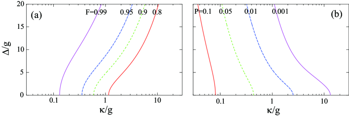
Figure 3: Contour plots of (a) fidelity and (b) success probability as functions of the cavity decay rate $\kappa$ and the detuning $\Delta$ in units of the cavity coupling strength $g$. $\gamma_{p}=\gamma=2g$. Even when $\kappa=2g$, high-fidelity operation (${\cal F}=0.9$) is possible by setting $\Delta=9g$. The success probability will then be ${\cal P}=0.13$%.

Finally, we describe a possible experimental realization of our scheme using NV centers. In a cavity QED setup composed of a diamond NV center and a microtoroidal cavity, the parameters $g$, $\kappa$, and $\gamma$ have comparable values of the order of tens of MHz Park et al. (2006), while $\gamma_{p}$ is highly sensitive to temperature Fu et al. (2009). The linewidth of the NV center will be almost lifetime limited and thus $\gamma_{p}$ will be negligible at low temperatures such as $7$ K, whereas $\gamma_{p}$ will dominate the other parameters at higher temperatures. At a low temperature ($\gamma_{p}=0.1g$ and $\gamma=g$), ${\cal F}=0.96$ can be attained with ${\cal P}=0.13\%$ even by a low Q cavity ($\kappa=4g$ and $\Delta=5g$). Thus, using our scheme, it should be possible to realize an EO using current technology. Moreover, even at higher temperatures, it should be possible to perform an EO by our scheme with modest requirements that are expected to be achievable in the near future. Here, we set the parameters as $\gamma_{p}/2\pi=300$ MHz (which corresponds to a temperature of about $30$ K Fu et al. (2009)), $\gamma/2\pi=20$ MHz, $g/2\pi=250$ MHz, $\kappa/2\pi=150$ MHz, and $\Delta/2\pi=3$ GHz. Entanglement can be generated with ${\cal F}=0.90$ and ${\cal P}=0.96\%$. In principle, once this amount of remote entanglement is achieved between distant nodes, one can realize scalable distributed quantum computation by using purification techniques inside the nodes Goyal et al. (2006); Fujii et al. (2012). Therefore, distributed quantum computation may be possible at temperatures of tens of kelvins, which can easily be generated without using liquid helium Daibo et al. (2011); Felder et al. (2010).

In conclusion, we performed a non-perturbative analysis of an EO using a detuned photon as a mediator between optically active matter qubits. We demonstrated that this scheme is extremely robust against environmental noise so that entanglement can be generated between homogeneously broadened matter qubits even in the weak-coupling regime, where damping parameters overwhelm the coherent coupling between the cavity and the qubit. This result is particularly relevant for realizing distributed quantum computation by using NV centers at high temperatures of the order of tens of kelvins. Our scheme provides a practical way to overcome the main obstacle of using NV centers at high temperatures, namely large homogeneous broadening.

The authors thank H. Kosaka and W. J. Munro for helpful discussions. This work was supported in part by the Funding Program for World-Leading Innovative R&D on Science and Technology (FIRST), KAKENHI (22241025, 23104710, and 22244035), SCOPE (111507004), and NICT Commissioned Research.

Appendix A cavity-QED analysis of single-photon dynamics

A.1 Hamiltonian and initial state vector

We present here mathematical details on time evolution of a single input photon in the proposed optical circuit. To begin with, we analyze transmission of a photon through a cavity. The physical setup is illustrated in Fig. 4. It is composed of (i) a matter qubit, which has three levels ($|0\rangle$, $|1\rangle$, $|e\rangle$), (ii) a two-sided cavity, (iii) leak fields from the cavity ($b$ and $b^{\prime}$ fields), (iv) noncavity radiation modes ($d$ field), and (v) environmental modes causing pure dephasing of the qubit ($e$ field). Since the state $|0\rangle$ is optically inactive, we may regard the qubit as a two-level system ($|1\rangle$, $|e\rangle$) when investigating its optical response. Putting $\hbar=c=1$, the Hamiltonian is given by

$${\cal H} = \omega_{q}\sigma^{\dagger}\sigma+\omega_{c}c^{\dagger}c+g(\sigma^{\dagger}c+c^{\dagger}\sigma)$$ (17)

$$+ \int dk\left[kb_{k}^{\dagger}b_{k}+\sqrt{\kappa/4\pi}(c^{\dagger}b_{k}+b_{k}^{\dagger}c)\right]+\int dk\left[kb_{k}^{\prime\dagger}b^{\prime}_{k}+\sqrt{\kappa/4\pi}(c^{\dagger}b^{\prime}_{k}+b_{k}^{\prime\dagger}c)\right]$$

$$+ \int dk\left[kd_{k}^{\dagger}d_{k}+\sqrt{\gamma/2\pi}(\sigma^{\dagger}d_{k}+d_{k}^{\dagger}\sigma)\right]+\int dk\left[ke_{k}^{\dagger}e_{k}+\sqrt{\gamma_{p}/\pi}\sigma^{\dagger}\sigma(e_{k}+e_{k}^{\dagger})\right],$$

where $\sigma(=|1\rangle\langle e|)$ and $c$ are the destruction operators of qubit and cavity photon, and $\alpha_{k}$ ($\alpha=b$, $b^{\prime}$, $d$, $e$) is the destruction operator of $\alpha$ field in the wavenumber representation. The meanings of the parameters are given in the main text. The field operator in the real-space representation is defined by $\widetilde{\alpha}_{r}=(2\pi)^{-1/2}\int dke^{ikr}\alpha_{k}$. The $r<0$ ($r>0$) region corresponds to the incoming (outgoing) field.

At the initial moment ($t=0$), we assume that a single photon is input from the $b$ field and all other components are in their ground state. The initial state vector is then written as

$$|\Psi_{in}\rangle=\int drf(r)\widetilde{b}_{r}^{\dagger}|1\rangle,$$ (18)

where $f(r)$ is the wavefunction of the input photon. It is assumed to be

$$f(r)=\sqrt{2/l}\ \theta(-r)\exp(i\omega_{p}r+r/l),$$ (19)

where $\theta(r)$ is the Heavyside step function. Namely, the input photon has a pulse length $l$ and a central frequency $\omega_{p}$.

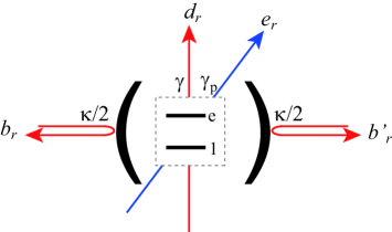
Figure 4: The cavity-QED setup considered. A matter qubit is confined in a two-sided cavity, and a single photon is input from the left-hand side.

A.2 Heisenberg equations

From the Hamiltonian of Eq. (17), the raw Heisenberg equation for $b_{k}$ is given by $db_{k}/dt=-ikb_{k}-i\sqrt{\kappa/4\pi}\ c$. This can be formally solved as $b_{k}(t)=b_{k}(0)e^{-ikt}-i\sqrt{\kappa/4\pi}\int_{0}^{t}d\tau c(\tau)e^{-ik(t-\tau)}$. As the Fourier transform of this equation, $\widetilde{b}_{r}(t)$ is given by

$$\widetilde{b}_{r}(t)=\widetilde{b}_{r-t}(0)-i\sqrt{\kappa/2}\theta(r)\theta(t-r)c(t-r).$$ (20)

Similarly, we have

$$\widetilde{b}^{\prime}_{r}(t) = \widetilde{b}^{\prime}_{r-t}(0)-i\sqrt{\kappa/2}\theta(r)\theta(t-r)c(t-r),$$ (21)

$$\widetilde{d}_{r}(t) = \widetilde{d}_{r-t}(0)-i\sqrt{\gamma}\theta(r)\theta(t-r)\sigma(t-r),$$ (22)

$$\widetilde{e}_{r}(t) = \widetilde{e}_{r-t}(0)-i\sqrt{2\gamma_{p}}\theta(r)\theta(t-r)\sigma^{\dagger}(t-r)\sigma(t-r).$$ (23)

These equations are known as the input-output relations. The Heisenberg equations for $\sigma$ and $c$ are given by

$$\frac{d}{dt}\sigma = -i\widetilde{\omega}_{q}\sigma-ig(1-2\sigma^{\dagger}\sigma)c-i\sqrt{\gamma}(1-2\sigma^{\dagger}\sigma)\widetilde{d}_{-t}(0)-i\sqrt{2\gamma_{p}}[\widetilde{e}_{-t}^{\dagger}(0)\sigma+\sigma\widetilde{e}_{-t}(0)],$$ (24)

$$\frac{d}{dt}c = -i\widetilde{\omega}_{c}c-ig\sigma-i\sqrt{\kappa/2}[\widetilde{b}_{-t}(0)+\widetilde{b}^{\prime}_{-t}(0)],$$ (25)

where $\widetilde{\omega}_{q}=\omega_{q}-i(\gamma/2+\gamma_{p})$ and $\widetilde{\omega}_{c}=\omega_{c}-i\kappa/2$.

In the main text, the input and output fields ($a_{in}$, $a^{\prime}_{in}$, $a_{out}$, $a^{\prime}_{out}$) are defined as shown in Fig. 2. They are related to the $b$ and $b^{\prime}$ fields as $a_{in}(t)=\widetilde{b}_{-t}(0)$, $a^{\prime}_{in}(t)=\widetilde{b}^{\prime}_{-t}(0)$, $a_{out}(t)=\widetilde{b}_{+0}(t)$ and $a^{\prime}_{out}(t)=\widetilde{b}^{\prime}_{+0}(t)$. After making these replacements, Eqs. (3)–(6) of the main text are derived.

A.3 Correlation functions

We discuss here the following one-time correlation functions, $\alpha_{q}(t)=\langle 1|\sigma(t)\sigma^{\dagger}|1\rangle$, $\alpha_{c}(t)=\langle 1|c(t)\sigma^{\dagger}|1\rangle$, $\beta_{q}(t)=\langle 1|\sigma(t)|\Psi_{in}\rangle$ and $\beta_{c}(t)=\langle 1|c(t)|\Psi_{in}\rangle$. Their initial conditions are given by $\alpha_{q}(0)=1$ and $\alpha_{c}(0)=\beta_{q}(0)=\beta_{c}(0)=0$. From Eqs. (24) and (25), their equations of motion are given by

$$\frac{d}{dt}\left[\begin{array}[]{c}\alpha_{q}(t)\\ \alpha_{c}(t)\end{array}\right] = \left[\begin{array}[]{cc}-i\widetilde{\omega}_{q}&-ig\\ -ig&-i\widetilde{\omega}_{c}\end{array}\right]\left[\begin{array}[]{c}\alpha_{q}(t)\\ \alpha_{c}(t)\end{array}\right],$$ (32)

$$\frac{d}{dt}\left[\begin{array}[]{c}\beta_{q}(t)\\ \beta_{c}(t)\end{array}\right] = \left[\begin{array}[]{cc}-i\widetilde{\omega}_{q}&-ig\\ -ig&-i\widetilde{\omega}_{c}\end{array}\right]\left[\begin{array}[]{c}\beta_{q}(t)\\ \beta_{c}(t)\end{array}\right]+\left[\begin{array}[]{c}0\\ -i\sqrt{\frac{\kappa}{2}}f(-t)\end{array}\right].$$ (41)

We denote the Laplace transform of $\alpha_{q}(t)$ by ${\cal L}_{\alpha_{q}}(z)=\int_{0}^{\infty}dte^{-zt}\alpha_{q}(t)$. Then, the Laplace transforms of the above equations are given by

$$\left[\begin{array}[]{c}{\cal L}_{\alpha_{q}}(z)\\ {\cal L}_{\alpha_{c}}(z)\end{array}\right] = \frac{1}{(z-\lambda_{1})(z-\lambda_{2})}\left[\begin{array}[]{c}z+i\widetilde{\omega}_{c}\\ -ig\end{array}\right],$$ (46)

$$\left[\begin{array}[]{c}{\cal L}_{\beta_{q}}(z)\\ {\cal L}_{\beta_{c}}(z)\end{array}\right] = \frac{-i\sqrt{\kappa/l}}{(z-\lambda_{1})(z-\lambda_{2})(z-\lambda_{3})}\left[\begin{array}[]{c}-ig\\ z+i\widetilde{\omega}_{q}\end{array}\right],$$ (51)

where $\lambda_{1}$ and $\lambda_{2}$ are the two roots of $(z+i\widetilde{\omega}_{q})(z+i\widetilde{\omega}_{c})+g^{2}=0$ and $\lambda_{3}=-1/l-i\omega_{p}$. The one-time correlation functions are obtained by analyzing the poles of the above Laplace transforms.

Next, we proceed to discuss the two-time functions such as $\beta^{(2)}_{q}(t_{1},t_{2})=\langle 1|\sigma(t_{1})\sigma^{\dagger}(t_{2})\sigma(t_{2})|\Psi_{in}\rangle$ and $\beta^{(2)}_{c}(t_{1},t_{2})=\langle 1|c(t_{1})\sigma^{\dagger}(t_{2})\sigma(t_{2})|\Psi_{in}\rangle$, where $t_{1}>t_{2}$. Their equations of motion with respect to $t_{1}$ are the same as Eq. (32), and the initial conditions ($t_{1}\to t_{2}$) are given by $\beta^{(2)}_{q}(t_{2},t_{2})=\beta_{q}(t_{2})$ and $\beta^{(2)}_{c}(t_{2},t_{2})=0$. Therefore, we have

$$\beta^{(2)}_{q}(t_{1},t_{2}) = \alpha_{q}(t_{1}-t_{2})\beta_{q}(t_{2}),$$ (52)

$$\beta^{(2)}_{c}(t_{1},t_{2}) = \alpha_{c}(t_{1}-t_{2})\beta_{q}(t_{2}).$$ (53)

Repeating the same logic, general multi-time functions are written as the products of one-time functions as

$$\beta^{(n)}_{q}(t_{1},\cdots,t_{n}) = \alpha_{q}(t_{1}-t_{2})\alpha_{q}(t_{2}-t_{3})\cdots\beta_{q}(t_{n-1}-t_{n}),$$ (54)

$$\beta^{(n)}_{c}(t_{1},\cdots,t_{n}) = \alpha_{c}(t_{1}-t_{2})\alpha_{q}(t_{2}-t_{3})\cdots\beta_{q}(t_{n-1}-t_{n}).$$ (55)

A.4 Wavefunctions of transmitted photon

After interaction with the qubit-cavity system, the input photon is reflected into the $b$ field, transmitted into the $c$ field, or scattered into the $d$ field. Time evolution of the input photon is determined by $|\Psi(t)\rangle=e^{-i{\cal H}t}|\Psi_{in}\rangle$. The state vector of the transmitted component of photon is written as

$$|\Psi_{c}(t)\rangle=\left[\int drg_{0}(r,t)\widetilde{b}_{r}^{\prime\dagger}+\int drdx_{1}g_{1}(r,x_{1},t)\widetilde{b}_{r}^{\prime\dagger}\widetilde{e}_{x_{1}}^{\dagger}+\cdots\right]|1\rangle.$$ (56)

Note that $0<r<x_{1}<\cdots<t$. $g_{0}$ describes the elastic component, whereas $g_{n}$ ($n\geq 1$) describes the inelastic component that is entangled with the environmental modes ($e_{x}^{\dagger}$). We can determine $g_{0}$ as follows: $g_{0}(r,t)=\langle 1|\widetilde{b}^{\prime}_{r}|\Psi_{c}(t)\rangle=\langle 1|\widetilde{b}^{\prime}_{r}(t)|\Psi_{in}\rangle=-i\sqrt{\kappa/2}\beta_{c}(t-r)$, where Eq. (21) is used to derive the last equality. Repeating the same arguments, we have

$$g_{0}(r,t) = -i\sqrt{\kappa/2}\beta_{c}(t-r),$$ (57)

$$g_{1}(r,x_{1},t) = (-i\sqrt{\kappa/2})(-i\sqrt{2\gamma_{p}})\beta_{q}(t-x_{1})\alpha_{c}(x_{1}-r),$$ (58)

$$g_{n}(r,x_{1},\cdots,x_{n},t) = (-i\sqrt{\kappa/2})(-i\sqrt{2\gamma_{p}})^{n}\beta_{q}(t-x_{n})\alpha_{q}(x_{n}-x_{n-1})\cdots\alpha_{c}(x_{1}-r).$$ (59)

On the other hand, when the qubit is in $|0\rangle$, the photon does not interact with the qubit and inelastic processes are absent accordingly. The state vector of the transmitted photon is then written as

$$|\overline{\Psi}_{c}(t)\rangle = \int dr\overline{g}_{0}(r,t)\widetilde{b}_{r}^{\prime\dagger}|0\rangle,$$ (60)

where $\overline{g}_{0}(r,t)=\lim_{g\to 0}g_{0}(r,t)$.

A.5 Fidelity and success probability

Here we investigate the density matrix of matter qubits after an entanglement operation. Throughout this section, we denote the photon field operator in the left (right) arm of the interferometer by $a_{Lr}$ ($a_{Rr}$). The initial state vector is $|\psi_{i}\rangle=2^{-1}\int drf(r)a_{Lr}^{\dagger}[|00\rangle+|01\rangle+|10\rangle+|11\rangle]$. The beamsplitters divide a photon as $a_{Lr}^{\dagger}\to(ia_{Lr}^{\dagger}+a_{Rr}^{\dagger})/\sqrt{2}$ and $a_{Rr}^{\dagger}\to(ia_{Rr}^{\dagger}+a_{Lr}^{\dagger})/\sqrt{2}$, and the qubit-cavity system transforms a photon as Eqs. (56)–(60). When the photon is output in the left port of BS2, the state vector of the overall system is given by

$$|\Psi_{L}\rangle = \frac{1}{\sqrt{8}}\int dr\left[\overline{g}_{0}(r,t)-g_{0}(r,t)\right]\widetilde{a}_{Lr}^{\dagger}|\phi_{t}\rangle,$$ (61)

$$- \frac{1}{\sqrt{8}}\sum_{n=1}^{\infty}\int drdx_{1}\cdots dx_{n}g_{n}(r,x_{1},\cdots,x_{n},t)\widetilde{a}_{Lr}^{\dagger}\widetilde{e}_{Rx_{1}}^{\dagger}\cdots\widetilde{e}_{Rx_{n}}^{\dagger}|\phi_{e1}\rangle,$$ (62)

$$+ \frac{1}{\sqrt{8}}\sum_{n=1}^{\infty}\int drdx_{1}\cdots dx_{n}g_{n}(r,x_{1},\cdots,x_{n},t)\widetilde{a}_{Lr}^{\dagger}\widetilde{e}_{Lx_{1}}^{\dagger}\cdots\widetilde{e}_{Lx_{n}}^{\dagger}|\phi_{e2}\rangle,$$ (63)

where $|\phi_{t}\rangle=(|01\rangle-|10\rangle)/\sqrt{2}$ is the target entangled state, $|\phi_{e1}\rangle=(|01\rangle+|11\rangle)/\sqrt{2}$, and $|\phi_{e2}\rangle=(|10\rangle+|11\rangle)/\sqrt{2}$.

The success probability ${\cal P}$ of the entanglement operation, namely, the probability to click the detector, is given by ${\cal P}=\langle\psi_{L}|\psi_{L}\rangle$. Denoting the norm of a function $f$ by ${\cal N}(f)$, we have

$${\cal P}={\cal N}(\overline{g}_{0}-g_{0})/8+\sum_{n=1}^{\infty}{\cal N}(g_{n})/4.$$ (64)

The reduced density matrix $\rho$ of matter qubits is defined by $\rho={\rm Tr}_{a,e}|\psi_{L}\rangle\langle\psi_{L}|/\langle\psi_{L}|\psi_{L}\rangle$. Therefore,

$$\rho=\frac{{\cal N}(\overline{g}_{0}-g_{0})|\phi_{t}\rangle\langle\phi_{t}|+\sum_{n=1}^{\infty}{\cal N}(g_{n})(|\phi_{e1}\rangle\langle\phi_{e1}|+|\phi_{e2}\rangle\langle\phi_{e2}|)}{{\cal N}(\overline{g}_{0}-g_{0})+2\sum_{n=1}^{\infty}{\cal N}(g_{n})}.$$ (65)

The fidelity ${\cal F}$ between $\rho$ and the target state $|\phi_{t}\rangle\langle\phi_{t}|$ is given by

$${\cal F}=\frac{{\cal N}(\overline{g}_{0}-g_{0})+\sum_{n=1}^{\infty}{\cal N}(g_{n})/2}{{\cal N}(\overline{g}_{0}-g_{0})+\sum_{n=1}^{\infty}2{\cal N}(g_{n})}.$$ (66)

It is of note that the infinite sum of $\sum_{n=1}^{\infty}{\cal N}(g_{n})$ can be carried out analytically. Using the Laplace transforms of $|\alpha_{c}|^{2}$, $|\alpha_{q}|^{2}$ and $|\beta_{q}|^{2}$, we have

$$\sum_{n=1}^{\infty}{\cal N}(g_{n})=\kappa\gamma_{p}\frac{{\cal L}_{|\beta_{q}|^{2}}(0){\cal L}_{|\alpha_{c}|^{2}}(0)}{1-2\gamma_{p}{\cal L}_{|\alpha_{q}|^{2}}(0)}.$$ (67)

In the long pulse limit of $l\to\infty$, ${\cal N}(\overline{g}_{0}-g_{0})$ and $\sum_{n=1}^{\infty}{\cal N}(g_{n})$ respectively reduce to $|1-t_{e}|^{2}$ and $|t_{i}|^{2}$ as discussed in the main text.

Appendix B numerical results

In this section we present the numerical results that are not presented in the main text. We assume $\omega_{p}=\omega_{c}$ throughout this section and denote the qubit-cavity detuning $\omega_{q}-\omega_{c}$ by $\Delta$.

B.1 Pulse Length

First, we observe the effects of a finite pulse length $l$ of an input photon. Assuming a dissipation-free ($\gamma=\gamma_{p}=0$) and resonant ($\Delta=0$) case, the success probability ${\cal P}$ is plotted as a function of $l$ for several values of $\kappa$ in Fig. 5(a). We can observe there that ${\cal P}$ becomes independent of $l$ for $l\gg\kappa^{-1}$ and reaches the limit value given by Eq. (16) of main text. This implies that the long-pulse limit, where the input photon can enter the cavity perfectly, is achieved when the spectral width of input photon ($l^{-1}$) is much narrower than that of cavity ($\kappa$). For shorter pulses, the cavity filters out the off-resonant components of input photon and the success probability is decreased accordingly. In the short-pulse region, the success probability becomes proportional to $l$ since it is determined by the overlap between the spectra of input photon and cavity.

Figure 5(b) shows the $l$-dependence of fidelity. As expected, ${\cal F}$ becomes independent of $l$ in the long-pulse limit and the limit value is given by Eq. (15) of the main text. However, in contrast with Fig. 5(a), the fidelity is insensitive to $l$ also in the short pulse region. This can be understood intuitively as follows. Once the photon enters the cavity, its property is determined by the cavity linewidth and becomes irrelevant to the original linewidth determined by $l$. We can observe that both the success probability and the fidelity are maximized in the long pulse limit.

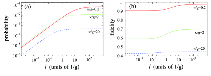
Figure 5: Dependences of (a) success probability and (b) fidelity on the input pulse length $l$. $\gamma=\gamma_{p}=0$ and $\Delta=0$. The values of $\kappa$ are indicated in the figure.

B.2 Spontaneous Emission

Here we observe the effects of nonzero $\gamma$. Assuming a noisy environment ($\gamma_{p}=2g$) and a resonant input photon ($\Delta=0$), the fidelity ${\cal F}$ is plotted as a function of $\kappa$ and $\gamma$ in Fig. 6(a). We can confirm that the cavity condition is substantially relaxed by a nonzero $\gamma$. In order to achieve ${\cal F}=0.9$ for example, $\kappa=0.08g$ is required when $\gamma$ is absent, whereas this condition is relaxed to $\kappa=0.59g$ when $\gamma=2g$. Usually, spontaneous emission into irrelevant modes leads to dissipation of quantum devices and lowers their figure of merits. However, this is not the case with the present scheme. The origin of infidelity here is inelastic scattering (in other words, entanglement with environment), which occurs while the qubit is being excited. Spontaneous emission makes the lifetime of excited state shorter and thus hinders inelastic scattering. The success probability ${\cal P}$ is shown in Fig. 6(b). It is observed that ${\cal P}$ is lowered by $\gamma$. Thus, a high-fidelity operation becomes possible at the expense of a lower success probability.

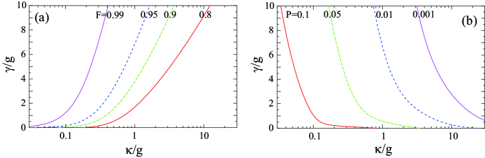
Figure 6: Contour plots of (a) fidelity and (b) success probability, as functions of $\kappa$ and $\gamma$. $\gamma_{p}=2g$ and $\Delta=0$.

References

Cirac et al. (1999)
J. I. Cirac,
A. K. Ekert,
S. F. Huelga,
and
C. Macchiavello,
Phys. Rev. A 59,
4249 (1999).
Barrett and Kok (2005)
S. D. Barrett and
P. Kok,
Phys. Rev. A 71,
060310 (2005).
Lim et al. (2005)
Y. Lim,
A. Beige, and
L. Kwek,
Phys. Rev. Lett. 95,
030505 (2005).
Browne et al. (2003)
D. E. Browne,
M. B. Plenio,
and S. F.
Huelga, Phys. Rev. Lett
91, 067901
(2003).
Bose et al. (1999)
S. Bose,
P. Knight,
M. Plenio, and
V. Vedral,
Phys. Rev. Lett. 83,
5158 (1999).
Feng et al. (2003)
X. Feng,
Z. Zhang,
X. Li,
S. Gong, and
Z. Xu, Phys.
Rev. Lett. 90, 217902
(2003).
Ladd et al. (2006)
T. Ladd,
P. Van Loock,
K. Nemoto,
W. Munro, and
Y. Yamamoto,
New J. Phys. 8,
184 (2006).
Van Loock et al. (2006)
P. Van Loock,
T. Ladd,
K. Sanaka,
F. Yamaguchi,
K. Nemoto,
W. Munro, and
Y. Yamamoto,
Physical review letters 96,
240501 (2006).
Azuma et al. (2009)
K. Azuma,
N. Sota,
R. Namiki,
Ş. Özdemir,
T. Yamamoto,
M. Koashi, and
N. Imoto,
Physical Review A 80,
060303 (2009).
Moehring et al. (2007)
D. L. Moehring,
P. Maunz,
S. Olmschenk,
K. C. Younge,
D. N. Matsukevich,
L.-M. Duan, and
C. Monroe,
Nature 449, 68
(2007).
Nielsen (2004)
M. Nielsen,
Phys. Rev. Lett. 93,
040503 (2004).
Duan and Raussendorf (2005)
L.-M. Duan and
R. Raussendorf,
Phys. Rev. Lett. 95,
080503 (2005).
Gross et al. (2006)
D. Gross,
K. Kieling, and
J. Eisert,
Phys. Rev. A 74,
042343 (2006).
Matsuzaki et al. (2010)
Y. Matsuzaki,
S. C.Benjamin,
and
J. Fitzsimons,
Phys. Rev. Lett 104,
4 (2010).
Raussendorf and Briegel (2001)
R. Raussendorf and
H. Briegel,
Phys. Rev. Lett. 86,
5188 (2001).
Benjamin et al. (2006)
S. C. Benjamin,
D. E. Browne,
J. Fitzsimons,
and J. J. L.
Morton, New J. Phys.
8, 141 (2006).
Togan et al. (2010)
E. Togan,
Y. Chu,
A. Trifonov,
L. Jiang,
J. Maze,
L. Childress,
M. Dutt,
A. Sørensen,
P. Hemmer,
A. Zibrov,
et al., Nature
466, 730 (2010).
Fu et al. (2009)
K. Fu,
C. Santori,
P. Barclay,
L. Rogers,
N. Manson, and
R. Beausoleil,
Phys. Rev. Lett. 103,
256404 (2009).
Childress et al. (2005)
L. Childress,
J. M. Taylor,
A. S. Sørensen,
and M. D. Lukin,
Phys. Rev. A 72,
052330 (2005).
Matsuzaki
et al. (2011a)
Y. Matsuzaki,
S. Benjamin, and
J. Fitzsimons,
Physical Review A 83,
060303 (2011a).
Matsuzaki
et al. (2011b)
Y. Matsuzaki,
P. Solinas, and
M. Möttönen,
Physical Review A 84,
032338 (2011b).
Sipahigil et al. (2011)
A. Sipahigil,
M. Goldman,
E. Togan,
Y. Chu,
M. Markham,
D. Twitchen,
A. Zibrov,
A. Kubanek, and
M. Lukin,
Arxiv preprint arXiv:1112.3975 (2011).
Elitzur and Vaidman (1993)
A. Elitzur and
L. Vaidman,
Foundations of Physics 23,
987 (1993).
Hornberger (2006)
K. Hornberger,
Arxiv preprint arXiv:0612118v3 (2006).
Park et al. (2006)
Y. Park,
A. Cook, and
H. Wang,
Nano letters 6,
2075 (2006).
Goyal et al. (2006)
K. Goyal,
A. McCauley, and
R. Raussendorf,
Phys. Rev. A 74,
032318 (2006).
Fujii et al. (2012)
K. Fujii,
T. Yamamoto,
M. Koashi, and
N. Imoto,
Arxiv preprint arXiv:1202.6588 (2012).
Daibo et al. (2011)
M. Daibo,
S. Fujita,
M. Haraguchi,
K. Kikuchi,
Y. Iijima, and
T. Saitoh,
Physica C: Superconductivity (2011).
Felder et al. (2010)
B. Felder,
M. Miki,
K. Tsuzuki,
M. Izumi, and
H. Hayakawa, in
Journal of Physics: Conference Series
(IOP Publishing, 2010), vol.
234, p. 032009.