Excursion set theory for modified gravity: correlated steps, mass functions and halo bias

Abstract

We show how correlated steps introduces significant contributions to the modification of the halo mass function in modified gravity models, taking the chameleon models as an example, in the framework of the excursion set approach. This correction applies to both Lagrangian and Eulerian environments discussed in previous studies. Correlated steps also enhances the modifications due to the fifth force in the conditional mass function as well as the halo bias. We found that abundance and clustering measurements from different environments can provide strong constraints on the chameleon models.

1 Introduction

The discovery of accelerated expansion of the Universe sparks surge of research on the possibility of modified gravity model (see, for example, Jain & Khoury, 2010; Clifton et al., 2012, for review). The main goal of such modification is to alter the large scale behaviour to explain the weakening of gravity – however any modifications in the gravity model must at the same time satisfy the tight constraints from the solar system test. One way to fullfill this requirement is to include some kinds of screening mechanisms to suppress the modification in local environment (high density regime). In this work we focus on one particular example – one that modifies gravity by introducing a dynamical scale field which mediates a fifth force. This scalar field has the nice property such that the fifth force is strongly suppressed in regions of high matter density and hence it passes the solar system test.

The chameleon model of Khoury & Weltman (2004); Mota & Shaw (2007) is a representative example (other noticeable examples are the environmentally dependent dilation Brax et al. (2010) and symmetron (Hinterbichler & Khoury, 2010) models). The background evolution and the linear perturbations on large scale can be indistinguishable from the standard $\Lambda$CDM cosmology (Hu & Sawicki, 2007; Li & Barrow, 2007; Brax et al., 2008; Li & Zhao, 2009); solar system test is satisfied by construction. Hence nonlinear structure formation is the only regime where effects of such models would possibly be detected. A number of studies (Oyaizu, 2008; Oyaizu et al., 2008; Schmidt et al., 2009; Li & Zhao, 2009, 2010; Li & Barrow, 2011; Zhao, Li & Koyama, 2011; Li et al., 2011; Brax et al., 2011; Davis et al., 2011) employed N-body numerical simulations to study nonlinear structure formation – however high resolution simulations with cosmological volume are still challenging due to the non linear equation governing the scalar field.

This work aims at investigating the effect of chameleon mechanism on large scale structure. We apply the excursion set approach (Bond et al., 1991; Mo & White, 1996; Sheth & Tormen, 1999) to compute the halo mass function in the same line as previous analyses done by Li & Efstathiou (2012); Li & Lam (2012). Li & Efstathiou (2012) first illustrated the idea of extending the excursion set approach to calculate halo mass function in chameleon models (see Brax, Rosenfeld & Sterr (2010) for an earlier work in this direction, where the authors studied the spherical collapse in chameleon models in detail). They did so by assuming a fixed Lagrangian environment. Li & Lam (2012) improved this approach by introducing an Eulerian environment. This choice avoids the unphysical requirement that all environments having the same mass (which also places an upper limit of the halo mass). The calculation involves two first crossing distributions, one for the Eulerian environment and the other one for the (modified) halo formation barrier. Both studies compute the effect of the chameleon mechanism assuming uncorrrelated steps in the excursion set approach – it is the main focus of the first half of the current work to investigate how correlated steps in the excursion set approach interact with the fifth force and the chameleon mechanism. Recently there are renewed interests in going beyond the uncorrelated steps excursion set in GR+$\Lambda$CDM cosmology to compute the halo/void abundance (Maggiore & Riotto, 2010; Paranjape, Lam & Sheth, 2012a, b; Musso & Sheth, 2012) and the halo bias (Ma et al., 2011; Paranjape & Sheth, 2012; Musso & Sheth, 2012).

In addition to the unconditional mass function, the excursion set approach lays down the framework to calculate the conditional mass function as well as the halo bias. The latter is of particular importance since it relates observables (distribution of halos) to the underlying matter distribution. Since the mass function in chameleon models depends on the environment density, one may expect the conditional mass function (and hence the halo bias) to be modified. The second part of this paper discusses how the conditional mass function as well as the halo bias depend on the chameleon model.

This paper is organised as follows: in § 2 we briefly review the theoretical model to be considered and summarise its main ingredients. The effect of the chameleon mechanism on the halo mass function within the framework of excursion set approach is presented in § 3, where we also include analytical approximation for correlated steps in § 3.4. § 4 discusses the conditional mass function and halo bias in chameleon models where we show measurements in underdense environment provide a good test for chameleon signatures. Finally we conclude in § 5.

2 The Chameleon Theory

This section lays down the theoretical framework for investigating the effects of coupled scalar field(s) in cosmology. We shall present the relevant general field equations in § 2.1, and then specify the models analysed in this paper in § 2.2.

2.1 Cosmology with a Coupled Scalar Field

The equations presented in this sub-section can be found in (Li & Zhao, 2009, 2010; Li & Barrow, 2011), and are presented here only to make this work self-contained.

We start from a Lagrangian density

$${\cal L}={1\over{2}}\left[{R\over\kappa}-\nabla^{a}\varphi\nabla_{a}\varphi\right]+V(\varphi)-C(\varphi){\cal L}_{\rm{DM}}+{\cal L}_{\rm{S}},$$ (1)

in which $R$ is the Ricci scalar, $\kappa=8\pi G$ with $G$ being the gravitational constant, ${\cal L}_{\rm{DM}}$ and ${\cal L}_{\rm{S}}$ are respectively the Lagrangian densities for dark matter and standard model fields. $\varphi$ is the scalar field and $V(\varphi)$ its potential; the coupling function $C(\varphi)$ characterises the coupling between $\varphi$ and dark matter. Given the functional forms for $V(\varphi)$ and $C(\varphi)$ a coupled scalar field model is then fully specified.

Varying the total action with respect to the metric $g_{ab}$, we obtain the following expression for the total energy momentum tensor in this model:

$$T_{ab} = \nabla_{a}\varphi\nabla_{b}\varphi-g_{ab}\left[{1\over 2}\nabla^{c}\nabla_{c}\varphi-V(\varphi)\right]$$ (2)

$$\quad+C(\varphi)T^{\rm{DM}}_{ab}+T^{\rm{S}}_{ab},$$

where $T^{\rm{DM}}_{ab}$ and $T^{\rm{S}}_{ab}$ are the energy momentum tensors for (uncoupled) dark matter and standard model fields. The existence of the scalar field and its coupling change the form of the energy momentum tensor leading to potential changes in the background cosmology and structure formation.

The coupling to a scalar field produces a direct interaction (fifth force) between dark matter particles due to the exchange of scalar quanta. This is best illustrated by the geodesic equation for dark matter particles

$${{{\rm d}^{2}\bf{r}}\over{{\rm d}t^{2}}}=-\vec{\nabla}\phi-{{C_{\varphi}(\varphi)}\over{C(\varphi)}}\vec{\nabla}\varphi,$$ (3)

where $\bf{r}$ is the position vector, $t$ the (physical) time, $\phi$ the Newtonian potential and $\vec{\nabla}$ is the spatial derivative. $C_{\varphi}\equiv{\rm d}C/{\rm d}\varphi$. The second term in the right hand side is the fifth force and only exists for coupled matter species (dark matter in our model). The fifth force also changes the clustering properties of the dark matter.

To solve the above two equations we need to know both the time evolution and the spatial distribution of $\varphi$, i.e. we need the solutions to the scalar field equation of motion (EOM)

$$\nabla^{a}\nabla_{a}\varphi+{{\rm{d}V(\varphi)}\over{\rm{d}\varphi}}+\rho_{\rm{DM}}{\frac{\rm{d}C(\varphi)}{\rm{d}\varphi}}=0,$$ (4)

or equivalently

$$\nabla^{a}\nabla_{a}\varphi+{{\rm{d}V_{eff}(\varphi)}\over{\rm{d}\varphi}}=0,$$ (5)

where we have defined

$$V_{eff}(\varphi)=V(\varphi)+\rho_{\rm{DM}}C(\varphi).$$ (6)

The background evolution of $\varphi$ can be solved easily given the present day value of $\rho_{\rm{DM}}$ since $\rho_{\rm{DM}}\propto a^{-3}$. We can then divide $\varphi$ into two parts, $\varphi=\bar{\varphi}+\delta\varphi$, where $\bar{\varphi}$ is the background value and $\delta\varphi$ is its (not necessarily small nor linear) perturbation, and subtract the background part of the scalar field equation of motion from the full equation to obtain the equation of motion for $\delta\varphi$. In the quasi-static limit in which we can neglect time derivatives of $\delta\varphi$ as compared with its spatial derivatives (which turns out to be a good approximation on galactic and cluster scales), we find

$$\vec{\nabla}^{2}\varphi={{\rm{d}C(\varphi)}\over{\rm{d}\varphi}}\rho_{\rm{DM}}-{{\rm{d}C(\bar{\varphi})}\over{\rm{d}\bar{\varphi}}}\bar{\rho}_{\rm{DM}}+{{\rm{d}V(\varphi)}\over{\rm{d}\varphi}}-{{\rm{d}V(\bar{\varphi})}\over{\rm{d}\bar{\varphi}}},$$ (7)

where $\bar{\rho}_{\rm{DM}}$ is the background dark matter density.

The computation of the scalar field $\varphi$ using the above equation then completes the computation of the source term for the Poisson equation

$$\vec{\nabla}^{2}\phi = \frac{\kappa}{2}\left[\rho_{\rm tot}+3p_{\rm tot}\right]$$ (8)

$$= {{\kappa}\over{2}}\left[C(\varphi)\rho_{\rm{DM}}+\rho_{\rm{B}}-2V(\varphi)\right],$$

where $\rho_{\rm{B}}$ is the baryon density (we have neglected the kinetic energy of the scalar field because it is always very small for the model studied here).

2.2 Specification of Model

As mentioned above, to fully fix a model we need to specify the functional forms of $V(\varphi)$ and $C(\varphi)$. Here we will use the models investigated by Li & Zhao (2009, 2010); Li (2011), with

$$C(\varphi)=\exp(\gamma\sqrt{\kappa}\varphi),$$ (9)

and

$$V(\varphi)={{\Lambda}\over{\left[1-\exp\left(-\sqrt{\kappa}\varphi\right)\right]^{\alpha}}}.$$ (10)

In the above $\Lambda$ is a parameter of mass dimension four and is of order the present dark energy density ($\varphi$ plays the role of dark energy in the models). $\gamma,\alpha$ are dimensionless parameters controlling the strength of the coupling and the steepness of the potentials respectively.

We shall choose $\alpha\ll 1$ and $\gamma>0$ as in Li & Zhao (2009, 2010), ensuring that $V_{eff}$ has a global minimum close to $\varphi=0$ and ${\rm d}^{2}V_{eff}(\varphi)/{\rm d}\varphi^{2}\equiv m^{2}_{\varphi}$ at this minimum is very large in high density regions. There are two consequences of these choices of model parameters: (1) $\varphi$ is trapped close to zero throughout cosmic history so that $V(\varphi)\sim\Lambda$ behaves as a cosmological constant; (2) the fifth force is strongly suppressed in high density regions where $\varphi$ acquires a large mass, $m^{2}_{\varphi}\gg H^{2}$ ($H$ is the Hubble expansion rate), and thus the fifth force cannot propagate far. The suppression of the fifth force is even stronger at early times, and thus its influence on structure formation occurs mainly at late times. The environment-dependent behaviour of the scalar field was first investigated by Khoury & Weltman (2004); Mota & Shaw (2007), and is often referred to as the ‘chameleon effect’.

3 First Crossing Probability with Correlated Steps in Chameleon Models

3.1 Terminology

In the excursion set approach the calculation of the halo mass function ${\rm d}n/{\rm d}m$ is mapped to the computation of the first crossing distribution $f(S)$ across some prescribed barriers where

$$\frac{m}{\bar{\rho}}\frac{{\rm d}n}{{\rm d}m}{\rm d}m=f(S){\rm d}S.$$ (11)

In the following we use the two terms interchangeably. The variance of the matter fluctuation field smoothed on scale $R$ is given by

$$S=\int\frac{{\rm d}k}{k}\frac{k^{3}P(k)}{2\pi^{2}}W^{2}(kR),$$ (12)

where $W$ is the smoothing window function and $P(k)$ is the matter power spectrum linear extrapolated to the present time. In hierarchical models $S$ is a monotonic decreasing function of $R$ and the smoothing scale in Lagrangian space $R$, the total mass enclosed within this scale $M$, and the variance $S$ are equivalent quantities and can be used interchangeably.

3.2 Background

Recent work (Li & Efstathiou, 2012; Li & Lam, 2012) demonstrated how the chameleon-type fifth force modifies the first crossing probability and the associated halo mass function for Lagrangian and Eulerian environment. This modification is due to the dependence of the halo formation barrier height $\delta_{c}(S)$ on the matter density of its surrounding environment, $\delta_{\rm env}$. Since the fifth force is strongest when the environment density is low, the barrier for halo formation is lower where $\delta_{\rm env}$ is small. The upper panel in figure 1 shows the halo formation barrier as a function of $S$ for various values of $\delta_{\rm env}$ assuming that the spherical collapse model describes halo formation, and confirms that the fifth force is stronger in underdense environment where the associated barrier is lower. The actual height that the random walks with various $\delta_{\rm env}$ need to climb to reach the modified barrier is shown in the lower panel – although the barrier in underdense environment is lower, the barrier to overcome is actually higher.

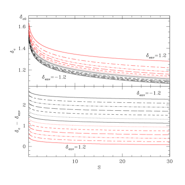
Figure 1: Upper panel: Halo formation barrier for various $\delta_{\rm env}$ from -1.2 to 1.2 with increment 0.2. Constant barrier at the top is the case with no fifth force (i.e., $\Lambda$CDM). Lower panel: The height need to climb to reach the halo formation barrier for various $\delta_{\rm env}$.

Li & Efstathiou (2012); Li & Lam (2012), when applying the excursion set approach in chameleon models, focused on the case where the excursion set is performed with uncorrelated steps with two different definitions of environment. In both cases the modifications in the first crossing distribution in chameleon models are solely due to the change in the barrier. The situation is more complicated when the steps in the random walk are correlated: two additional effects can modify the first crossing distribution. Firstly, the distribution of $\delta_{\rm env}$ for Eulerian environments is modified and, since the halo formation barrier depends on $\delta_{\rm env}$, the first crossing probability will be modified as well. Note however that when the environment is defined as Lagrangian, the distribution of $\delta_{\rm env}$ is unchanged. Secondly, there will be non-trivial correlations between the environment density contrast $\delta_{\rm env}$ and the density contrast $\delta$ at different $S$.

To investigate how these two effects modify the first crossing distribution in models with chameleon mechanism, we use monte-carlo simulations to study the first crossing distribution for three choices of smoothing window functions following the procedures in Bond et al. (1991). Our convention is such that the normalisation of the power spectrum is set by demanding $\sigma_{8}=0.81$ for the tophat filter. The sharp-k smoothing window function generates random walks with uncorrelated steps and it is common practice to use the $S-M$ mapping of the tophat window function to relate the variance and the smoothing scale for the sharp-k smoothing window function. We consider $\Lambda$CDM power spectrum and two environment scales: an Eulerian environment, which denoted by $\zeta$, is the environment at late time; and a Lagrangian environment, which denoted by $\xi$, is the environment in the initial conditions. We assume both environments are spherical regions that share common centers as the proto-halos. The actual scale of the environment should be approximately the Compton wavelength of the scalar field at late time. Numerical simulation results suggest that an Eulerian scale of $\zeta=5\sim 8h^{-1}{\rm Mpc}$ should be chosen (Li, Zhao & Koyama, 2012). In this work we consider an Eulerian evironment $\zeta=5h^{-1}$Mpc and a Lagrangian environment $\xi=8h^{-1}$Mpc, and set $(\gamma,\alpha)=(0.5,10^{-6})$ as the chameleon model parameters. In the language of excursion set formalism, the Lagrangian environment barrier (fixing $S$) corresponds to a vertical barrier in the $\delta_{l}-S$ plane while the Eulerian environment barrier is given by the spherical collapse model (Bernardeau, 1994; Sheth, 1998):

$$b_{\rm Eul}(S)=\delta_{c0}\left[1-\left(\frac{M(S)}{\bar{\rho}\zeta}\right)^{-1/\delta_{c0}}\right],$$ (13)

where $\bar{\rho}$ is the background density.

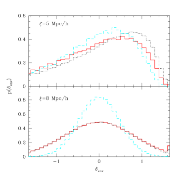
Figure 2: (Colour Online) Distribution of environmental density for Eulerian (top panel) and Lagrangian environments (lower panel). The solid, dashed and dotted curves are results of tophat, Gaussian and sharp-k window functions respectively.

Figure 2 shows the distribution of $\delta_{\rm env}$ for $\zeta=5\ {\rm Mpc}/h$ (upper panel) and $\xi=8\ {\rm Mpc}/h$ (lower panel). Three histograms corresponding to tophat (solid), Gaussian (dashed), and sharp-k (dotted) window functions are shown in each panel. We ran a sample of random walk whose correlation satisfies the corresponding smoothing filter function. We then record the height of the random walk at which it first crosses the environmental barrier. In the case of Lagrangian environment we set $\delta_{\rm env}=\delta_{c0}$ if the random walk first crosses $\delta_{c0}$ on scale bigger than $\xi$. Since we use the same $S-M$ mapping for the tophat window function and the sharp-$k$ window function, choosing a Lagrangian scale fixes $S$ and hence the two will have the same distribution. The difference between the distributions of Gaussian smoothing and the others in the case of Lagrangian environment is due to our choice of power spectrum normalization – for $\xi=8\ {\rm Mpc}/h$, $\lg(\nu)=1.1$ for the Gaussian filter while $\lg(\nu)=0.62$ for the tophat and sharp-k filters. Here $\nu\equiv\delta_{\rm c0}^{2}/S$. Since the Lagrangian $\delta_{\rm env}$ distribution is the same for the tophat and sharp-k filters, any difference in their first crossing distributions due to the fifth force has to come from the non-trivial correlations between the height of the random walk and $\delta_{\rm env}$ (see below). On the other hand, the distributions in Eulerian environment are different for all three smoothing windows: the sharp-k filter peaks at highest $\delta_{\rm env}$ while the Gaussian filter peaks at lowest $\delta_{\rm env}$. As a result the effect of the fifth force is stronger when the Gaussian window function is used – the halo formation barrier for walks with Gaussian filter is lower than that of uncorrelated walks. Analytical approximations to evaluate the first crossing of Eulerian environment are available for both uncorrelated (Zhang & Hui, 2006; Lam & Sheth, 2009) and correlated steps (Musso & Sheth, 2012).

3.3 Monte-Carlo simulations

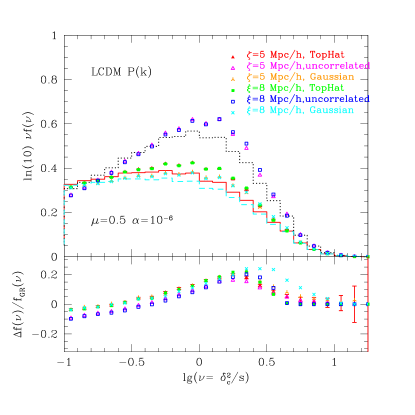
Figure 3: (Colour Online) Comparison of the first crossing distribution in chameleon models for correlated as well as uncorrelated steps. Three sets of histograms are the first crossing probability for the $\Lambda$CDM model, a constant barrier $\delta_{c}=1.676$, for different smoothing window functions: from top to bottom are sharp-k filter (uncorrelated walks), tophat filter, and Gaussian filter. The symbols are the first crossing distribution when there is the fifth force for $\zeta=5h^{-1}$Mpc and $\xi=8h^{-1}$Mpc. See the legends for the details. The bottom panel shows the fractional change in the first crossing probability with respect to the corresponding constant barrier first crossing probability. Only error bars for red solid triangles are included for clarity.

The top panel in figure 3 shows the first crossing distributions in chameleon models for both correlated and uncorrelated walks. The histograms show the distribution when there is no fifth force: it is the first crossing for a constant barrier at $\delta_{c}=1.676$. The line labels are the same as in figure 2. Symbols represent the first crossing distributions for different combinations of smoothing window functions and choices of environment, as indicated in the legends. The first crossing distributions change significantly when the random walks switch from uncorrelated steps (sharp-k) to the correlated one (Gaussian and tophat); different definitions of the environment have subdominant effect. To better visualise the effect of different choices of the environment, the lower panel shows the relative difference in the distribution to the corresponding constant barrier distribution.

The modifications in the first crossing distribution due to the chameleon-type fifth force are quite different for random walks with correlated steps (both Gaussian and tophat filters) versus walks with uncorrelated steps. For example the modifications of the correlated steps are displaced from those of the uncorrelated steps for $\lg(\nu)<0.1$. Since the modification in the halo mass function is around 20%, this $\sim 5$% displacement is a big contribution. Consider for example the tophat (solid squares) and the sharp-k (open squares) Lagrangian environments – since they have the same distribution $p(\delta_{\rm env})$, the difference in the predicted modification in the first crossing distributions must be due to the nontrivial correlations between different smoothing scales when the window function is tophat. One can imagine the following scenario: random walks with correlated steps are less likely to have dramatic fluctuations compared to those with uncorrelated steps – when $\delta_{\rm env}<0$, the enhanced fifth force lowers the barrier $\delta_{c}$ – in both uncorrelated and correlated cases, it is easier to cross the barrier. However correlated walks are not likely have sudden jumps, hence the modification in the first crossing comes only at bigger $S$: it explains the difference between the solid (tophat Lagrangian) and open (sharp-k Lagrangian) symbols for $\lg(\nu)>0.3$ (Lagrangian scale $\xi=8\ {\rm Mpc}/h$ corresponds to $\lg(\nu)=0.62$). For bigger $S$ the correlated walks do not need have sudden jumps to cross the barrier – hence the increase in the first crossing probability. On the other hand, the increase for the uncorrelated walks is smaller since some of those walks already cross the barrier at smaller $S$. For $\delta_{\rm env}>0$, the fifth force is weak and only slightly enhances structure formation. In this case walks with correlated steps may upcross the barrier sooner than walks with uncorrelated steps (since uncorrelated walks can have sudden decrease in height). It will result in higher probability in first crossing distribution for correlated steps for $S$ near the chameleon environment – however this modification in the first crossing distribution relative to the GR case is small due to the weakening of the fifth force. Recall that it is equally likely to have overdense and underdense environment in Lagrangian environment, the net effect is correlated steps show a smaller change in first crossing probability for small $s$ but bigger change for big $s$.

The change in first crossing distribution for Gaussian filter and Lagrangian environment is strong in high $\nu$. It is consistent with the change in the distribution of $\delta_{\rm env}$ shown in figure 2: since $p(\delta_{\rm env})$ has a narrower distribution with a peak at $\delta_{\rm env}=0$, the overdense environments in the Gaussian case generally have lower $\delta_{\rm env}$ and so the fifth force is stronger (lower barrier) compared to the walks with tophat or sharp-k filter. On the other hand the change at low mass end is similar to others – although there are more walks that have underdense Lagrangian environments for the other two filters, those walks need to climb a huge distance to cross their respective modified barriers and do not make a significant contribution in the first crossing distribution.

3.4 Analytical approximation

In this subsection we apply the analytical approximation proposed by Musso & Sheth (2012) to estimate the first crossing distribution in chameleon models. In this analytical approximation the first crossing probability at $s$ is approximated by both the height and its rate of change at $s-\Delta s$. The first crossing distribution across barrier $b(s)$ is

$$f(s)=p(b,s)\int_{b^{\prime}}^{\infty}{\rm d}\delta^{\prime}\ p(\delta^{\prime}|b,s)(\delta^{\prime}-b^{\prime}),$$ (14)

where the dash denotes derivative with respect to $s$, $p(\delta^{\prime}|b,s)$ is the conditional probability density of the rate of change in height $\delta^{\prime}$ at $s$ given that the walk’s height is $b$ at the same scale $s$, and $p(\delta,s)$ is the probability density that the walk has height $b$ at the smoothing scale $s$.

When the Lagrangian environment is used in the chameleon models, the first crossing distribution of the modified barrier $b=\delta_{c}(s,\delta_{\rm env})$ at $s$ is

$$f_{\rm Lag}(s;\xi) = \int_{-\infty}^{\delta_{c0}}{\rm d}\delta_{\rm env}\ p(\delta_{\rm env},\xi)p(b,s|\delta_{\rm env},\xi)$$ (15)

$$\times\int_{b^{\prime}}^{\infty}{\rm d}\delta^{\prime}\ p(\delta^{\prime}|b,s;\delta_{\rm env},\xi)(\delta^{\prime}-b^{\prime}),$$

where $p(\delta_{\rm env},\xi)$ is the distribution of environmental density contrast at scale $\xi$. Strictly speaking $p(\delta_{\rm env},\xi)$ should be replaced by the condition probability that $\delta$ never crosses $\delta_{c0}$ for scales bigger than $\xi$, but the scales we apply the Lagrangian environment is big enough so that the difference between the two is small.

Figure 4 shows the comparison of the analytical approximation and the monte-carlo results for Lagrangian environment of $\xi=8{\rm Mpc}/h$. The upper panel shows the results of Gaussian window function while the lower panel shows the tophat window function. In each panel the top half shows the first crossing distribution from analytical prediction (curve) and the monte-carlo result (symbols), and the bottom half shows the modifications to the first crossing distribution relative to GR. The analytical approximation matches the monte-carlo simulation for $\lg(\nu)>0$ – for smaller $\nu$, multiple crossings are more frequent and the approximation breaks down.

Figure 4: Analytical approximation for first crossing distribution in chameleon models for correlated steps. The upper and the lower figure show the results using Lagrangian environment $\xi=8\ {\rm Mpc}/h$ for Gaussian and tophat window filters respectively. In each figure the curve is the analytical approximation while the data points are monte-carlo simulation results. The upper half of each figure shows the first crossing distribution and the lower half shows the ratio to the constant barrier distribution. The vertical dotted lines show the scales of the Lagrangian environment.

The first crossing distribution for Eulerian environment contains two first crossings: first to cross the environment barrier, then the halo formation barrier. Applying the approximation to both crossings yields

$$f_{\rm Eul}(s,\zeta) = \int_{0}^{s}{\rm d}S\ p(B,S)\int_{B^{\prime}}^{\infty}{\rm d}\Delta^{\prime}\ p(\Delta^{\prime}|B,S)(\Delta^{\prime}-B^{\prime})$$ (16)

$$\times p(b,s|B,S;\Delta^{\prime})$$

$$\quad\times\int_{b^{\prime}}^{\infty}{\rm d}\delta^{\prime}\ p(\delta^{\prime}|b,s;B,S;\Delta^{\prime})(\delta^{\prime}-b^{\prime}),$$

where we denote the Eulerian environment barrier as $B(S)$ and $\Delta^{\prime}$ is the derivative of $\delta_{\rm env}$ at $S$. The dependence of the halo barrier $b(s)$ on $B(S)$ is implicit. The first integral includes walks with different Eulerian environment density contrast (up to $s$) while the second integral corresponds to the first crossing of the Eulerian barrier at $S$. Here one should have replaced the upper limit of the integration such that the walk would not cross $\delta_{c0}$ at $S$ – in practice the probability of having a big jump is not likely so using the above approximation does not alter the result. Finally the rest corresponds to the first crossing of the modified halo barrier at $s$ given the walk first crossed the Eulerian barrier at $S$ with an increase in height $\Delta^{\prime}$ when going from $S-\Delta S$ to $S$. The results are shown in figure 5.

Figure 5: Similar to figure 4 but using Eulerian environment $\zeta=5\ {\rm Mpc}/h$.

The analytical approximation works relatively well for big $\nu$ ($>1$) but breaks down for small $\nu$, as in the case of Lagrangian environment.

The conditional probability distributions in this subsection are also Gaussian distributed with mean and variance given by

$${\rm E}(x|y_{1},y_{2},\cdots,y_{n}) = \sum_{i,j=1}^{n}\langle xy_{i}\rangle A_{ij}^{-1}y_{j}$$ (17)

$${\rm Var}(x|y_{1},y_{2},\cdots,y_{n}) = {\rm Var}(x)-\sum_{j=1}^{n}\langle xy_{j}\rangle^{2}A_{jj}^{-1}$$ (18)

$$-2\sum_{j>k}\langle xy_{j}\rangle\langle xy_{k}\rangle A_{jk}^{-1},$$

where $A$ is the covariance matrix of $\{y_{i}\}$ and we assume all variables have unconditional means vanish in the above formuale.

4 Conditional Mass Function and Halo Bias in Chameleon Models

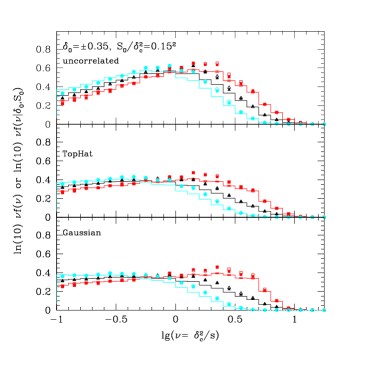
(a) $\delta_{0}=\pm 0.35$

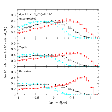
(b) $\delta_{0}=\pm 0.7$

Figure 6: (Colour Online) Comparison of the conditional first crossing probability obtained from Monte Carlo simulations for uncorrelated and correlated steps by selecting subset of walks that have various values of $\delta_{0}$ at $S_{0}=0.15^{2}\delta_{c}^{2}$. In each panel the histograms indicate the first crossing probability for the constant barrier case ($\Lambda$CDM) while the the solid symbols and the open symbols represent chameleon models with $\zeta=5h^{-1}$Mpc and $\xi=8h^{-1}$Mpc respectively. Three sets of probability are included in each panel: $|\delta_{0}|$ (highest amplitude histogram at $\lg(\nu)=0.5$ and squares); $-|\delta_{0}|$ (lowest amplitude histogram at $\lg(\nu)=0.5$ and pentagons); and unconditional probability (the intermediate histogram and triangles). Different panels use different smoothing window function: (from top to bottom): uncorrelated steps; tophat window function; Gaussian window function. Only error bars for the histogram for positive $\delta_{0}$ are included for clarity.

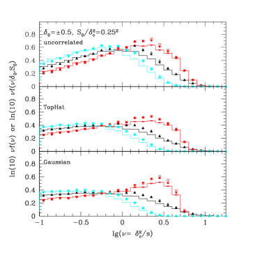
(a) $\delta_{0}=\pm 0.5$

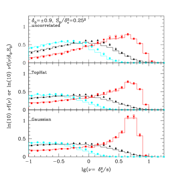
(b) $\delta_{0}=\pm 0.9$

Figure 7: (Colour Online) Conditional first crossing probability similar to figure 6 the condition is set at $S=0.25^{2}\delta_{c}^{2}$.

In this section we will describe the effect of the chameleon-type fifth force on the conditional mass function and the halo bias. As explained in the previous section, the fifth force is stronger when the environment is less dense – effectively the halo formation criterion is lower and hence the first crossing of halo formation barrier is easier. One may then ask if this effect will be more significant when we look at the conditional mass function, especially for underdense regions. Here we will use Monte Carlo simulations to investigate how the conditional mass function responses to the fifth force introduced by the chameleon models.

We now have two environments: one is used to solve the fifth force in the chameleon model (we will call it the chameleon environment hereafter and we choose $\zeta=5h^{-1}$Mpc and $\xi=8h^{-1}$Mpc) and the other is a large-scale environment $S=S_{0}$ on which the condition is defined. We will choose $S_{0}$ to be small (hence very large scale) so that it is safe to assume that the range of the fifth force is much smaller than the scale corresponding to $S_{0}$.

4.1 Conditional first crossing probability in chameleon models

In this subsection we will look at the conditional first crossing probability for three different smoothing window functions. The conditional first crossing probability is

$$f(S|\delta_{0},S_{0})=\int{\rm d}\delta_{\rm env}\ f(S|\delta_{\rm env};\delta_{0},S_{0})P(\delta_{\rm env}|\delta_{0},S_{0}),$$ (19)

where $f(S|\delta_{\rm env};\delta_{0},S_{0})$ is the conditional first crossing probability across the $\delta_{c}(S,\delta_{\rm env})$ barrier given that it first crosses the environment barrier $B(s)$ at $\delta_{\rm env}$ and it has $\delta=\delta_{0}$ at $S_{0}$. $P(\delta_{\rm env}|\delta_{0},S_{0})$ is the conditional first crossing probability of crossing the environment barrier at $\delta_{\rm env}$. Changing the large scale environment can have two effects:

1. It modifies the distribution of $\delta_{\rm env}$: when $\delta_{0}<0$, it is more likely to have less dense chameleon environment ($\delta_{\rm env}$ is smaller) and hence the fifth force will be stronger.

2. It also affects the first crossing distribution of the halo formation barrier when the random walk is non-Markovian (this effect is additional to the first point where the halo formation barrier is changed due to the change of environment distribution).

One may expect the second effect to be weaker than the first since the correlation is weaker for bigger difference in $S$. In particular, for sharp-k filter where the random walks have uncorrelated steps, the walks are Markovian and the large scale environment $(\delta_{0},S_{0})$ only modifies the distribution of $\delta_{\rm env}$, that is,

$$f_{\rm uncor}(S|\delta_{\rm env};\delta_{0},S_{0})=f(S|\delta_{\rm env}).$$ (20)

We are going to quantify the effect in this section using monte-carlo simulations. We choose two large scales ($S_{0}=0.15^{2}\delta_{c0}^{2}$ and $0.25^{2}\delta_{c0}^{2}$) and measure the conditional first crossing distributions using different window filters.

Figures 6 and 7 show the conditional first crossing distributions for various choices of $\delta_{0}$ at $S_{0}=0.15^{2}\delta_{c}^{2}$ and $0.25^{2}\delta_{c}^{2}$ respectively. In each panel the histograms indicate the first crossing probability for the constant barrier case ($\Lambda$CDM), while the solid and the open symbols represent chameleon models with $\zeta=5\ {\rm Mpc/h}$ and $\xi=8\ {\rm Mpc}/h$ respectively. Three sets of distribution are included in each panel: conditional probability with $\delta_{0}>0$ (highest amplitude histogram at $\lg(\nu)=0.5$ and squares), conditional probability with $\delta_{0}<0$ (lowest amplitude histogram at $\lg(\nu)=0.5$ and pentagons), and unconditional probability (the intermediate histogram and triangles). Different panels use different smoothing window functions, from top to bottom: sharp-k, tophat, and Gaussian filters. The conditional mass function differs from the unconditional mass function and the change depends on smoothing window function as well as the large scale density contrast $\delta_{0}$: in general conditional distributions using Gaussian or tophat window functions and having more extreme values of $\delta_{0}$ show more significant changes compared to the respective unconditional distribution.

The large scale environment modifies the distribution of the linear density contrast at the chameleon environment, which in turn modifies the first crossing distribution. The modification depends on the smoothing window functions due to the difference in correlation strength between various scales involved (the large scale environment, the chameleon environment, as well as the scale at which the halo barrier is first crossed). We took the ratio of the change in first crossing distribution for conditional walks to that of the unconditional walks and the results are shown in figure 8 and 9 for $\delta_{0}=\pm 0.5$ and $\pm 0.9$ respectively when $S_{0}=0.25^{2}\delta_{c0}^{2}$. The upper and lower panels of the two figures show respectively Eulerian environment and Lagrangian environment for the chameleon models. In each panel the ratios for $\delta_{0}<0$ are shifted upwards by 0.1 and symbols represent different smoothing window kernels: open symbols for sharp-k, solid symbols for tophat, and starred symbols for Gaussian.

If the change in the first crossing probability induced by the chameleon-type fifth force did not depend on the large scale environment, this ratio should be unity (indicated by the dotted horizontal line). The ratio above (below) unity indicates that those walks experience stronger (weaker) chameleon effect compared to the unconditional walks. They also make relative bigger (smaller) contributions to the change in the unconditional first crossing distribution. The monte-carlo results are consistent with expectations: for walks that have slightly overdense large scale environment ($\delta_{0}>0$), the ratio is always less than unity – these walks are more likely to have overdense $\delta_{\rm env}$ (regardless of the choice of Eulerian or the Lagrangian environment) and hence the strength of the fifth force is weaker. The ratios for walks with correlated steps (solid and starred triangles) have bigger deviations from unity compared to the ratio for walks with uncorrelated steps (open triangles), indicating the conditional distribution of $\delta_{\rm env}$ has stronger correlations with $\delta_{0}$ when steps are correlated (otherwise the correlation between $\delta_{0}$ and $\delta$ at some bigger $s$ should result in more first crossing). When the value of $\delta_{0}$ is more extreme, the deviations from unity is bigger indicating further weakening of the fifth force.

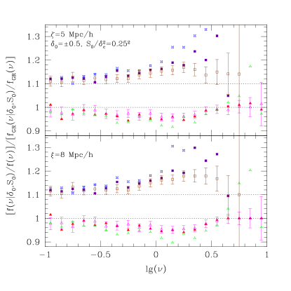
Figure 8: (Colour Online) Comparison of how the change in first crossing probability due to the fifth force depends on large scale environment $(\delta_{0},S_{0})$. The ratio are taken from the conditional distributions of figure 7a and compared to ratio taken from the unconditional distributions. The upper panel shows results with Eulerian environment $\zeta=5\ {\rm Mpc}/h$ and the lower panel is Lagrangian environment $\xi=8\ {\rm Mpc}/h$. Two sets of points in each panel indicate $\delta_{0}=0.5$ (lower set) and $\delta_{0}=-0.5$ (upper set, shifted by +0.1) respectively. Each set has three symbols representing different window functions: open (uncorrelated walks), solid (tophat), starred (Gaussian). Only error bars for uncorrelated walks are included as an approximate error indicator.

Figure 9: (Colour Online) Conditional first crossing probability similar to figure 8 (note the change in y-axis range) but the subsets of walks pass through $\delta_{0}=\pm 0.9$.

On the other hand for walks that have underdense large scale environment ($\delta_{0}<0$), the ratio for both uncorrelated and correlated walks stays above unity: the change in the first crossing distribution due to the fifth force is stronger than the unconditional walks. The ratio goes significantly above unity for correlated steps – indicating the abundance of intermediate mass halos in underdense environment would potentially provide a strong constraint on the chameleon-type fifth force.

Figure 10 shows a similar plot but with the large scale environment set at $S_{0}=0.15^{2}\delta_{c0}^{2}$. Comparison to figure 8 indicates that while the conditional distribution $p(\delta_{\rm env}|\delta_{0},S_{0})$ still differs from the unconditional distribution $p(\delta_{\rm env})$, the difference is less significant – very large environment ($S_{0}=0.15^{2}\delta_{c0}^{2}$) has weaker correlations with the chameleon environment compared to the previous case where $S_{0}=0.25^{2}\delta_{c0}^{2}$.

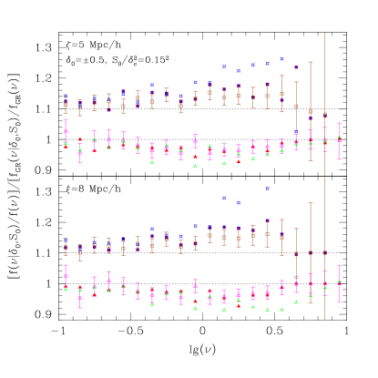
Figure 10: (Colour Online) Conditional first crossing probability similar to figure 8 but the subsets of walks pass through $\delta_{0}=\pm 0.5$ at $S_{0}=0.15^{2}\delta_{c0}^{2}$.

In this subsection we have studied the conditional mass function in chameleon models. The correlation between the large scale environment and the chameleon environment induces further modifications in the first crossing distribution – this effect is strongest (in terms of the modification of the conditional mass function) when the large scale environment is underdense. The corresponding change in the halo mass function for intermediate mass halo shows an extra $\sim$30% boost compared to the unconditional mass function. It is straightforward to extend the analytical approximation in § 3.4 to obtain the conditional first crossing distribution by including an additional condition $(\delta_{0},S_{0})$ in all the probability distributions in equations (15) and (16). This is beyond the scope of this work.

4.2 Halo bias in chameleon models

Halo bias describes the relationship between the halo overdensity $\delta_{h}$ and the matter overdensity $\delta$ where the halo overdensity can be expanded as

$$\delta_{h}=\sum_{i=1}\frac{b_{i}}{i!}\delta^{i}.$$ (21)

On large scale the above expansion can be truncated in the first few orders. In particular the linear bias term $b_{1}$ is commonly used to fit the ratio between the halo-matter power spectrum $P_{h\delta}$ and the matter power spectrum $P_{\delta\delta}$ (or its square as the ratio between halo power spectrum $P_{hh}$ and $P_{\delta\delta}$). The excursion set approach provides a natural way to relate halo abundance and halo bias – by starting the random walks at some prescribed locations rather the origin (Mo & White, 1996; Sheth & Tormen, 1999). The relative difference of this conditional first crossing probability to the unconditional one gives the left hand side of equation (21).

Recently there are several studies (Ma et al., 2011; Paranjape & Sheth, 2012) on evaluating the halo bias using the excursion set approach with correlated steps. Both of the analyses (using very different methods) found that the halo bias with correlated steps is stronger than the uncorrelated case. Paranjape & Sheth (2012) also suggests that, when correlated steps are considered, the halo bias computed from the excursion set approach is different from the one obtained by taking the ratio of the halo-matter power spectrum and the matter power spectrum. While we are interested in computing the halo bias with correlated steps, we do not make the distinction here and we will present the halo bias evaluated within the excursion set framework.

In the chameleon models the halo formation barrier in the excursion set approach depends on the environment density. To estimate the halo bias we use the conditional first crossing distributions obtained in the previous subsection and compute the halo bias from equation (21) where

$$b_{1}\delta_{c0}=\left[\frac{f(S|\delta_{0},S_{0})}{f(S)}-1\right]\frac{\delta_{c0}}{\delta_{0}},$$ (22)

assuming high order terms can be neglected. We chose the conditional first crossing distribution where $S_{0}=0.15^{2}\delta_{c0}^{2}$ and $\delta_{0}=\pm 0.35$ and $\pm 0.5$ and the results are shown in figure 11. The three panels show results using different smoothing window functions and the results for chameleon models are shifted by $\pm 4$.

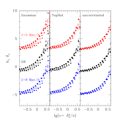
Figure 11: (Colour Online) Halo bias computed from monte-carlo simulations using equation (22). We chose $S_{0}=0.15^{2}\delta_{c0}^{2}$ and $\delta_{0}=\pm 0.35\ {\rm(solid)\ or}\ \pm 0.5\ {\rm(open)}$ for the conditional first crossing distribution where triangles (squares) represent positive (negative) $\delta_{0}$.

Halo bias using more correlated window functions has stronger dependence on the value of $\delta_{0}$, which can be seen by comparing the spread of bias among the three panels. Including the chameleon-type fifth force modifies the halo bias and their relative changes are shown in figure 12 and 13 for the Eulerian and Lagrangian environments respectively. In both environment definitions the relative difference of the halo bias in chameleon models can be of factor of a few, regardless of the window functions used. Another noticeable signature is the difference of the mass range where the halo bias relative difference is most significant: when the tophat or Gaussian window filters are used, the change in halo bias for most overdense environment (triangles, $\delta_{0}=0.5$) is most significant around $\lg(\nu)=-0.1$ but it is shifted to lower mass $\lg(\nu)=-0.5$ for underdense environment (solid lines, $\delta_{0}=-0.5$). This difference in mass range is getting smaller when $\delta_{0}$ is less extreme (see the difference between squares and dotted lines for $\delta_{0}=\pm 0.35$). Combining the measurements of the halo bias in very overdense and underdense environments to the GR predictions (analytical formula or measurements from numerical simulations) would probably constrain the chameleon models.

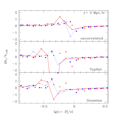
Figure 12: (Colour Online) Relative difference in halo bias for chameleon models (Eulerian environment) to that of GR. Triangles and solid lines are the relative difference for $\delta_{0}=\pm 0.5$ respectively; squares and dotted lines for $\delta_{0}=\pm 0.35$.

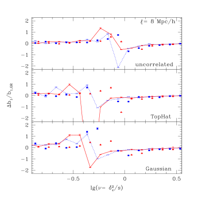
Figure 13: (Colour Online) Relative difference in halo bias for chameleon models (Lagrangian environment) to that of GR.

5 Conclusions

In this paper we investigated the modifications in the mass function and the halo bias due to the fifth force in the framework of excursion set approach. Two different environment definitions (Eulerian environment at $\zeta=5\ {\rm Mpc}/h$ and Lagrangian environment $\xi=8{\rm Mpc}/h$) are combined with three different smoothing window functions: Gaussian, tophat, and sharp-k, to study how correlations between different scales induced by the window functions interact with the fifth force.

The halo formation barrier in the chameleon model depends on the environment density $\delta_{\rm env}$ – in an accompanied paper (Li & Lam, 2012) we discussed the change in the mass function for Eulerian environment versus Lagrangian environment for uncorrelated steps (i.e. sharp-k window filter) using the excursion set approach. In that case the difference in the two environments only modifies the distribution of $\delta_{\rm env}$ and subsequently the first crossing distribution. Additional effect due to the non-trivial correlations between different smoothing scales arises when the smoothing function is Gaussian or tophat. We used monte-carlo simulations to demonstrate the additional correlations indeed modify the first crossing distribution and the contribution is significant, particularly in intermediate to low mass range. We then applied the analytical formalism proposed in Musso & Sheth (2012) to compute the first crossing distribution for correlated steps. The analytical prediction matches the monte-carlo simulations well for high mass regime.

Having shown the significance of correlated steps in the unconditional first crossing distribution, we examined the conditional mass function in chameleon models. When the steps in the excursion set are uncorrelated, the condition that random walks having passed through some $\delta_{0}$ at a prescribed large scale $S_{0}$ only alters the distribution of $\delta_{\rm env}$ due to the Markovian nature of uncorrelated steps. Correlated steps (the random walk is non-Markovian) introduce an additional effect due to the non-trivial correlations between $S_{0}$ and all other scales. We compared the change in the first crossing distribution due to the fifth force for conditional walks to that of unconditional walks and found that walks in underdense large scale environment experience a stronger modification compared to those in overdense large scale environment – this effect is observed in all the three smoothing window functions (with different strengths) usually used in the literature. Hence combining the conditional halo mass function in underdense large scale environment with the unconditional mass function can potentially provide a strong probe for modified gravity.

Finally we investigate how the chameleon models modify the halo bias derived from the excursion set approach. We found that the fifth force can modify the halo bias by a factor of a few at intermediate to low mass halos when underdense large scale environment is assumed. In addition we found that, when the correlated steps are used, the masses at which the halo bias is modified by the chameleon-type fifth force can be quite different for overdense and underdense environments. While this difference depends on the value of $\delta_{0}$, we found that $\Delta\lg(\nu)=0.4$ when $\delta_{0}$ at 2-$\sigma$ level for $S_{0}=0.15^{2}\delta_{c0}$.

The effect of the correlations between different smoothing scales introduced by the use of different smoothing window functions on halo abundance and halo bias has been the focus of some the recent studies. Its application with the excursion set approach in the chameleon models results in further modifications in both halo abundance and the halo bias. In particular the change in the conditional mass function and the halo bias in underdense environment may provide potentially strong constraints on the chameleon models. Another test we are investigating is the strength of correlations between the halo formation and the surrounding environment by measuring halo abundance and clustering under different environments in numerical simulations of chameleon models. This will be left for future study.

References

- Bernardeau (1994) Bernardeau F., 1994, ApJ, 427, 51
- Bond et al. (1991) Bond J. R., Cole S., Efstathiou G., Kaiser N., 1991, ApJ, 379, 440
- Brax, Rosenfeld & Sterr (2010) Brax P., Rosenfeld R., Steer D. A., 2010, JCAP, 08, 033
- Brax et al. (2008) Brax P., van de Bruck C., Davis A. C., Shaw D. J., 2008, PRD, 78, 104021
- Brax et al. (2010) Brax P., van de Bruck C., Davis A. C., Shaw D. J., 2010, PRD, 82, 063519
- Brax et al. (2011) Brax P., van de Bruck C., Davis A. C., Li B., Shaw D. J., 2011, PRD, in press
- Clifton et al. (2012) Clifton, T., Ferreira, P. G., Padilla, A., Skordis, C., 2012, PhR, 513, 1
- Davis et al. (2011) Davis A. C., Li B., Mota D. F., Winther H. A., 2011, arXiv:1108.3082 [astro-ph.CO]
- Hinterbichler & Khoury (2010) Hinterbichler K., Khoury J., 2010, PRL, 104, 231301
- Hu & Sawicki (2007) Hu W., Sawicki I., 2007, PRD, 76, 064004
- Jain & Khoury (2010) Jain B., Khoury J., 2010, Annals of Physics, 325, 1479
- Khoury & Weltman (2004) Khoury J., Weltman A., 2004, PRD, 69, 044026
- Lam & Sheth (2008a) Lam T. Y., Sheth R. K., 2008a, MNRAS, 386, 407
- Lam & Sheth (2008b) Lam T. Y., Sheth R. K., 2008b, MNRAS, 389, 1249
- Lam & Sheth (2009) Lam T. Y., Sheth R. K., 2009, MNRAS, 398, 2143
- Li (2011) Li B., 2011, MNRAS, 411, 2615
- Li & Barrow (2007) Li B., Barrow J. D., 2007, PRD, 75, 084010
- Li & Barrow (2011) Li B., Barrow J. D., 2011, PRD, 83, 024007
- Li & Efstathiou (2012) Li B., Efstathiou G., MNRAS, in press; arXiv:1110.6440 [astro-ph.CO]
- Li, Zhao & Koyama (2012) Li B., Zhao G.-B., Koyama K., 2012, MNRAS, in press; arXiv:1111.2602 [astro-ph.CO]
- Li & Zhao (2009) Li B., Zhao H., 2009, PRD, 80, 044027
- Li & Zhao (2010) Li B., Zhao H., 2010, PRD, 81, 104047
- Li et al. (2011) Li B., Zhao G., Teyssier R., Koyama K., 2011, arXiv:1110.1379 [astro-ph.CO]
- Li & Lam (2012) Li B., Lam T. Y., 2012, MNRAS, submitted; arXiv:1205:0058 [astro-ph.CO]
- Ma et al. (2011) Ma C., Maggiore M., Riotto A., Zhang J., 2011, MNRAS, 411, 2644
- Maggiore & Riotto (2010) Maggiore M., Riotto A., 2010, ApJ, 711, 907
- Mo & White (1996) Mo H. J., White S. D. M., 1996, MNRAS, 282, 347
- Mota & Shaw (2007) Mota D. F., Shaw, D. J., 2007, PRD, 75, 063501
- Musso & Sheth (2012) Musso M., Sheth R. K., 2012, arXiv:1201.3876
- Oyaizu (2008) Oyaizu H., 2008, PRD, 78, 123523
- Oyaizu et al. (2008) Oyaizu H., Lima M., Hu W., 2008, PRD, 78, 123524
- Paranjape & Sheth (2012) Paranjape A., Sheth R. K., 2012, MNRAS, 419, 132
- Paranjape, Lam & Sheth (2012a) Paranjape A., Lam T. Y., Sheth R. K., 2012, MNRAS, 420, 1429
- Paranjape, Lam & Sheth (2012b) Paranjape A., Lam T. Y., Sheth R. K., 2012, MNRAS, 420, 1648
- Schmidt et al. (2009) Schmidt F., Lima M., Oyaizu H., Hu W., 2009, PRD, 79, 083518
- Sheth (1998) Sheth R. K., 1998, MNRAS, 300, 1057
- Sheth & Tormen (1999) Sheth R. K., Tormen G., 1999, MNRAS, 308, 119
- Zhang & Hui (2006) Zhang J., Hui L., 206, ApJ, 641, 641
- Zhao, Li & Koyama (2011) Zhao G., Li B., Koyama K., 2011, PRD, 83, 044007