Abstract

Anomalously light fermionic partners of the top quark often appear in explicit constructions, such as the 5d holographic models, where the Higgs is a light composite pseudo Nambu-Goldstone boson and its potential is generated radiatively by top quark loops. We show that this is due to a structural correlation among the mass of the partners and the one of the Higgs boson. Because of this correlation, the presence of light partners could be essential to obtain a realistic Higgs mass.

We quantitatively confirm this generic prediction, which applies to a broad class of composite Higgs models, by studying the simplest calculable framework with a composite Higgs, the Discrete Composite Higgs Model. In this setup we show analytically that the requirement of a light enough Higgs strongly constraints the fermionic spectrum and makes the light partners appear.

The light top partners thus provide the most promising manifestation of the composite Higgs scenario at the LHC. Conversely, the lack of observation of these states can put strong restrictions on the parameter space of the model. A simple analysis of the $7$-TeV LHC searches presently available already gives some non-trivial constraint. The strongest bound comes from the exclusion of the $5/3$-charged partner. Even if no dedicated LHC search exists for this particle, a bound of $611$ GeV is derived by adapting the CMS search of bottom-like states in same-sign dileptons.

1 Introduction

The hints of a light Higgs boson have never been so strong. On top of the indirect indications coming from the ElectroWeak Precision Tests (EWPT) of LEP we now have powerful direct constraints from the LHC searches of ATLAS [1] and CMS [2]. As of today, a SM-like Higgs boson is constrained in a very narrow interval around $120$ GeV. Moreover, a promising excess has been found by both experiments at $m_{H}\simeq 125$ GeV, a reasonable expectation is that this excess will be confirmed by the 2012 LHC data and the Higgs will be finally discovered.

Very little can be said, on the contrary, about the nature of the Higgs. Minimality suggests that it should be an elementary weakly coupled particle, described by the Higgs model up to very high energy scales. Naturalness requires instead that a more complicated structure emerges around the TeV. A natural Higgs could still be elementary, if it is embedded in a supersymmetric framework, or it could be a composite object, i.e. the bound state of a new strong dynamics. In the latter case the Hierarchy Problem is solved by the finite size of the Higgs, which screens the contributions to its mass from virtual quanta of short wavelength. A particularly plausible possibility is that the Higgs is not a generic bound state of the strong dynamics, but rather a (pseudo) Nambu-Goldstone Boson (pNGB) associated to a spontaneously broken symmetry. This explains naturally why it is much lighter than the other, unobserved, strong sector resonances.

The idea of a composite pNGB Higgs has been studied at length [3, 4, 5, 6, 7, 8, 9, 10, 11, 12], and the following scenario has emerged. Apart from the Higgs, which is composite, all the other SM particles originate as elementary fields, external to the strong sector. The communication with the Higgs and the strong dynamics, and thus the generation of masses after ElectroWeak Symmetry Breaking (EWSB), occurs through linear couplings of the elementary fields with suitable strong sector operators. At low energies, below the confinement scale, the linear couplings become mixing terms among the elementary SM particles and some heavy composite resonance. The physical states after diagonalization possess a composite component, realizing the paradigm of “partial compositeness” [13, 6]. The simplest setup, which is almost universally adopted in the literature, is based on the ${\textrm{SO}}(5)\rightarrow{\textrm{SO}}(4)$ symmetry breaking pattern. This delivers only one pNGB Higgs doublet and incorporates the custodial symmetry to protect $\delta\rho$ from unacceptably large corrections. A possible model-building ambiguity comes from the choice of the ${\textrm{SO}}(5)$ representation of the fermionic operators that mix with the SM fermions and in particular with the third family $q_{L}$ and $t_{R}$. In the “minimal” scenario, often denoted as “MCHM5” in the literature, these operators are in the fundamental (${\mathbf{5}}$) representation. Other known possibilities are the ${\mathbf{4}}$ (MCHM4) and the ${\mathbf{10}}$ representations. Even if in the present paper we will adopt the minimal scenario as a reference, our results have a more general valence and range of applicability. We will discuss in the Conclusions the effect of changing the representations and of even more radical deformations.

Associated with the fermionic operators, massive colored fermionic resonances emerge from the strong sector. These are the so-called “top partners” and provide a very promising direct experimental manifestation of the composite Higgs scenario at the LHC [14]. Indeed it has been noticed by many authors, and in Ref. [5] for the first time, that in explicit concrete models these particles are anomalously light, much lighter than the other strong sector’s resonances. Concretely, one finds that the partners can easily be below $1$ TeV, with an upper bound of around $1.5$ TeV, while the typical strong sector’s scale is above $3$ TeV in order to satisfy the EWPT constraints. Moreover, Ref. [5] observed a certain correlation of the mass of the partners with the one of the Higgs boson.

The first goal of our paper will be to show that the lightness of the top partners has a structural origin, rather than being a peculiarity of some explicit model. The point is that in the composite Higgs scenario there is a tight relation among the top partners and the generation of the Higgs potential. This leads to a parametric correlation among the mass of the partners and the one of the Higgs boson. In order for the latter to be light as implied by the present data, we find that at least one of the top partners must be anomalously light. In section 2 we will describe this mechanism in detail by adopting a general description of the composite Higgs scenario with partial compositeness developed in ref.s [4, 6, 7]. Our results will thus have general validity and they will apply, in particular, to the 5d holographic models of ref.s [4, 5].

For a quantitative confirmation of the effect we need to study a concrete realization of the composite Higgs idea. The simplest possibility is to consider a “Discrete” Composite Higgs Model (DCHM) like the one proposed by two of us in Ref. [8]. The central observation behind the formulation of the DCHM is that the potential of the composite Higgs is saturated by the IR dynamics of the strong sector. Indeed in the UV, above the mass of the resonances which corresponds to the confinement scale, the Higgs “dissolves” in its fundamental constituents and the contributions to the potential get screened, as mentioned above. The same screening must take place in the low energy effective description of the theory and therefore the dynamics of the resonances must be such to give a finite and calculable (i.e., IR-saturated) Higgs potential. This is indeed what happens in the 5d holographic models thanks to the collective effect of the entire Kaluza-Klein tower. In the DCHM instead this is achieved by introducing a finite number of resonances and of extra symmetries which realize a “collective breaking” [15] protection of the Higgs potential. Further elaborations based on this philosophy can be found in Ref. [16]. Other models similar to the DCHM have been proposed in the context of Little-Higgs theories [17].

In sections 3 and 4 we describe in detail the structure of the top partners in the DCHM, and derive analytic explicit formulas that show quantitatively the correlation with the Higgs mass. Section 3 is devoted to the study of the 3-site DCHM, which provides a genuinely complete theory of composite Higgs. In this model, two layers of fermionic resonances are introduced and the Higgs potential is completely finite. In section 4 we consider instead a simpler but less complete model, the two-site DCHM. In this case one has a single layer of resonances and quite a small number ($3$, after fixing the top mass) of parameter describing the top partners. However the potential is not completely calculable, being affected by a logarithmic divergence at one loop [8]. Nevertheless it turns out that the divergence corresponds to a unique operator in the potential and therefore it can be canceled by renormalizing only one parameter which we can chose to be the Higgs VEV $v$. Thus, the Higgs mass is calculable also in the DCHM₂, this model can therefore be considered as the “simplest” composite Higgs model and it can be used to study the phenomenology of the top partners in correlation with the Higgs mass.

The analytic results are further supported by scatter plots, in which we scan all the available parameter space of the model. The results are quite remarkable: in the plane of the masses of the top partners the points with light enough Higgs boson fall very sharply in the region of light partners. Notice that the actual values of the partner’s mass is not fixed by our argument, it still depends on the overall mass scale of the strong sector. However this scale can only be raised at the price of fine-tuning the parameter $\xi\simeq(v/f_{\pi})^{2}$ (as defined in Ref. [7]) to very small values. Reasonable values of $\xi$, below which the entire scenario starts becoming unplausible, are $\xi=0.2$ or $\xi=0.1$. For $\xi=0.2$ we find that the partners are always below $1$ TeV while for $\xi=0.1$ the absolute maximum is around $1.5$ TeV. We therefore expect that the $14$-TeV LHC will have enough sensitivity to explore the parameter space of the model completely.

Non-trivial constraints can however already be obtained by the presently available exclusions from the $7$-TeV data, as we will discuss in section 5. The main effect comes from the exclusion of the 5/3-charged partner decaying to $tW^{+}$. No dedicated LHC search is available for this particle, however we find that it is possible to apply the bound of $611$ GeV coming from the CMS search of bottom-like heavy quarks in same-sign dileptons [18]. The bounds on the other partners are considerably reduced by the branching fractions to the individual decay channels assumed in the searches. We therefore expect that a significant improvement of the bounds could be obtained within some explicit model by combining the different channels. The $2$-site DCHM is definitely the best candidate, one might easily perform a complete scan of its $3$ free parameters. We have already implemented the $2$-site DCHM (and also of the $3$-site one) in MadGraph 5 [19] for the required simulations.

Finally, in section 6 we present our conclusion and an outlook of the possible implication of our results. In particular we discuss how our analysis could be adapted to more general scenarios of composite Higgs and we suggest some directions for future work.

2 Light Higgs wants light partners

If the Higgs is a pNGB its potential, and in particular its mass $m_{H}$, can only be generated through the breaking of the Goldstone symmetry. One unavoidable, sizable source of Goldstone symmetry breaking is the top quark Yukawa coupling $y_{t}$. Thus it is very reasonable to expect a tight relation among the Higgs mass and the fermionic sector of the theory which is responsible for the generation of $y_{t}$. This is particularly true in the canonical scenario of composite Higgs, summarized in the Introduction, where the only sizable contribution to the Higgs potential comes from the top sector. In more general cases there might be additional terms, coming for instance from extra sources of symmetry breaking not associated with the SM fermions and gauge fields [20]. Barring fine-tuning, the latter contributions can however at most enhance $m_{H}$, the ones from the top therefore provide a robust lower bound on the Higgs mass. If the Higgs has to be light, as it seems to be preferred by the present data, the top sector contribution must therefore be kept small enough by some mechanism. In the minimal scenario, as we will describe below, this is achieved by making anomalously light (and thus more easily detectable) some of the exotic states in the top sector.

In order to understand this mechanism we obviously need to specify in some detail the structure of the theory which controls the generation of $m_{H}$ and $y_{t}$. As anticipated in the Introduction, the paradigm adopted in the minimal model is the one of partial compositeness, in which the elementary left- and right-handed top fields are mixed with heavy vector-like colored particles, the so-called top partners. After diagonalization the physical top becomes an admixture of elementary and composite states and interacts with the strong sector, and in particular with the Higgs, through its composite component. The Yukawa coupling gets therefore generated and it is proportional to the sine of the mixing angles $\varphi_{L,R}$. The relevant Lagrangian, introduced in ref. [6], has the structure

$${\mathcal{L}}_{\textrm{mass}}\,=\,-\left(y_{L}f_{\pi}\,\overline{t}_{L}T_{R}+y_{R}f_{\pi}\,\overline{t}_{R}{\widetilde{T}}_{L}+{\textrm{h.c.}}\right)-m_{T}^{*}\overline{T}T-m_{\widetilde{T}}^{*}\overline{{\widetilde{T}}}{\widetilde{T}}\,,$$

$${\mathcal{L}}_{\textrm{Yuk}}\,=\,Y_{*}h\overline{T}{\widetilde{T}}+{\textrm{h.c.}}\,,$$ (1)

where $h$ is the Higgs field (before EWSB, i.e. $h=v+\rho$) and we have employed the decay constant $f_{\pi}$ of the Goldstone boson Higgs for the normalization of the elementary–composite mixings. After diagonalization, neglecting EWSB, the top Yukawa reads

$$y_{t}\,=\,Y_{*}\sin\varphi_{L}\sin\varphi_{R}\,,\;\;\;\;\;{\textrm{with}}\;\;\;\;\;\;\;\;\left\{\begin{array}[]{l}\sin\varphi_{L}=\frac{y_{L}f_{\pi}}{m_{T}}\\ \sin\varphi_{R}=\frac{y_{R}f_{\pi}}{m_{\widetilde{T}}}\end{array}\right.\,,$$ (2)

where $m_{T,{\widetilde{T}}}=\sqrt{(m_{T,{\widetilde{T}}}^{*})^{2}+(y_{L,R}f_{\pi})^{2}}$ are the physical masses of the top partners. 

The essential point of making the partners light is that this allows to decrease the elementary–composite mixings $y_{L,R}$ while keeping $y_{t}$ fixed to the experimental value. Let us consider the case of comparable left- and right-handed mixings, $y_{L}\simeq y_{R}\equiv y$. This condition, as explained in the following (see also [8]), is enforced in the minimal model by the requirement of a realistic EWSB. We can also assume that $m_{T}^{*}$ and $m_{{\widetilde{T}}}^{*}$, while potentially small, are still larger than $y_{L}f_{\pi}$ and $y_{R}f_{\pi}$, the critical value after which eq. (2) saturates and there is no advantage in further decreasing the masses. Under these conditions eq. (2) gives

$$y^{2}\,=\,\frac{y_{t}}{Y_{*}}\frac{m_{T}m_{\widetilde{T}}}{f_{\pi}^{2}}\,,$$ (3)

which shows how $y^{2}$ decreases linearly with the mass of each partner.

The mixings ensure the communication among the strong sector, which is invariant under the Goldstone symmetry, and the elementary sector which is not. Therefore they break the symmetry and allow for the generation of the Higgs mass. It is thus intuitive that a reduction of their value, as implied by eq. (3) for light top partners, will lead to a decrease of $m_{H}$. To be quantitative, let us anticipate the result of the following section (see also [5] and [8]): $m_{H}$ can be estimated as

$$m_{H}\simeq\sqrt{\frac{3}{2}}\frac{y^{2}v}{\pi}\,,$$ (4)

where $v\simeq 246$ GeV is the Higgs VEV. This gives, making use of eq. (3)

$$m_{H}\simeq 4\sqrt{3}m_{t}\,\frac{m_{T}m_{\widetilde{T}}}{4\pi Y_{*}f_{\pi}^{2}}\,.$$ (5)

The above equation already shows the correlation among the Higgs and the top partner mass. Of course we still need to justify eq. (4) and for this we need the more detailed analysis of the following section.

There is however one important aspect which is not captured by this general discussion. We see from eqs. (3) and (5) that making both $m_{T}$ and $m_{\widetilde{T}}$ small at the same time produces a quadratic decrease of $y^{2}$ and thus of $m_{H}$. However this behavior is never found in the explicit models we will investigate in the following sections, the effect is always linear. The basic reason is that, due to the Goldstone nature of the Higgs, the coupling $Y_{*}$ defined in eq. (1) depends itself on the partners mass. Indeed all the interactions of a pNGB Higgs are controlled by the dimensional coupling $f_{\pi}$ and no independent Yukawa-like coupling $Y_{*}$ can emerge. By dimensional analysis on has $Y_{*}\simeq m_{T,\widetilde{T}}^{*}/f_{\pi}$ or more precisely, as we will also verify below, $Y_{*}\simeq{\textrm{max}}(m_{T}^{*},m_{\widetilde{T}}^{*})/f_{\pi}$. Thus if both masses become small one power of $m_{T,{\widetilde{T}}}$ in eqs. (3) and (5) is compensated by $Y_{*}$ and the effect remains linear.

2.1 General analysis

For a better understanding we need a slightly more careful description of our theory. In particular we must take into account the Goldstone boson nature of the Higgs which is instead hidden in the approach of ref. [6] adopted in the previous discussion. Following ref.s [4, 7] (see also [9]) we describe the Higgs as a pNGB associated with the ${\textrm{SO}}(5)\rightarrow{\textrm{SO}}(4)$ spontaneous breaking which takes place in the strong sector. We parametrize (see [8] for the conventions) the Goldstone boson matrix as

$$U=e^{i\frac{\sqrt{2}}{f_{\pi}}\Pi_{\widehat{a}}T^{\widehat{a}}}\,,$$ (6)

where $T^{\widehat{a}}$ are the broken generators and $\Pi_{\widehat{a}}$ the $4$ real Higgs components. The Goldstone matrix transforms under $g\in{\textrm{SO}}(5)$ as [21]

$$U\;\rightarrow\;g\cdot U\cdot h^{t}\left(\Pi;\,g\right)\,,$$ (7)

where $h$ is a non-linear representation of ${\textrm{SO}}(5)$ which however only lives in ${\textrm{SO}}(4)$. With our choice of the generators $h$ is block-diagonal

$$h\,=\,\left(\begin{array}[]{cc}h_{4}&0\\ 0&1\end{array}\right)\,,$$ (8)

with $h_{4}\in{\textrm{SO}}(4)$

The SM fermions, and in particular the third family quarks $q_{L}=(t_{L}\;b_{L})$ and $t_{R}$, are introduced as elementary fields and they are coupled linearly to the strong sector. In the UV, where ${\textrm{SO}}(5)$ is restored, we can imagine that the elementary–composite interactions take the form

$${\mathcal{L}}\, =\,y_{L}\left({\overline{q}}_{L}\right)^{\alpha}\Delta_{\alpha I}^{L}\left({\mathcal{O}}_{R}\right)^{I}\,+\,y_{R}\left({\overline{t}}_{R}\right)\Delta_{I}^{R}\left({\mathcal{O}}_{L}\right)^{I}\,+\,\textrm{h.c.}\,,$$ (9)

where the chiral fermionic operators ${\mathcal{O}}_{L,R}$ transform in a linear representation of ${\textrm{SO}}(5)$. In particular in the minimal model we take both ${\mathcal{O}}_{L}$ and ${\mathcal{O}}_{R}$ in the fundamental, ${\mathbf{5}}$. The tensors $\Delta^{L,R}$ are uniquely fixed by the need of respecting the SM ${\textrm{SU}}(2)\times{\textrm{U}}(1)_{Y}$ group embedded in ${\textrm{SO}}(5)$

$$\Delta^{L}_{\alpha I}\,=\,\frac{1}{\sqrt{2}}\left(\begin{array}[]{ccccc}\;0&\;0&\;1&-i&\;0\\ \;1&\;i&\;0&\;0&\;0\end{array}\right)\,,$$ (12)

$$\Delta^{R}_{I}\,=\,-i\left(0\;0\;0\;0\;1\right)\,.$$ (13)

Let us also define, for future use, the embedding in the ${\mathbf{5}}$ of $q_{L}$ and of $t_{R}$

$$\left(q_{L}^{\mathbf{5}}\right)^{I}\,=\,\left({\Delta^{L}}^{*}\right)^{\alpha I}\left(q_{L}\right)_{\alpha}=\frac{1}{\sqrt{2}}\left(\begin{array}[]{ccccc}b_{L}&-ib_{L}&\;\;t_{L}&\;it_{L}&\;\;0\end{array}\right)\,,$$ (15)

$$\left(t_{R}^{\mathbf{5}}\right)^{I}\,=\,\left({\Delta^{R}}^{*}\right)^{I}t_{R}=i\left(\begin{array}[]{ccccc}0&0&0&0&t_{R}\end{array}\right)\,.$$ (17)

The elementary–composite couplings obviously break the Goldstone symmetry ${\textrm{SO}}(5)$. However provided the breaking is small we can still obtain valuable information from the ${\textrm{SO}}(5)$ invariance by the method of spurions. The point is that the theory, including the UV mixings in eq. (9), is perfectly invariant if we transform not just the strong sector fields and operators but also the tensors $\Delta^{L}$ and $\Delta^{R}$. This invariance survives in the IR description, the effective operators must therefore respect ${\textrm{SO}}(5)$ if we treat $\Delta^{L}$ and $\Delta^{R}$ as spurions which transform, formally, in the ${\mathbf{5}}$ of ${\textrm{SO}}(5)$. To be precise there are further symmetries one should take into account. These are the “elementary” ${\textrm{U}}(2)^{0}_{L}$ and ${\textrm{U}}(1)^{0}_{R}$, under which the strong sector is invariant and only the elementary fermions and the spurions transform. Certain linear combinations of the elementary group generators with the ${\textrm{SO}}(5)$ (and ${\textrm{U}}(1)_{X}$, see footnote 4) ones correspond to the SM group, these are of course preserved by the mixings.

The Higgs potential

Let us first discuss the implications of the spurionic analysis on the structure of the Higgs potential. We must classify the non-derivative invariant operators involving the Higgs and the spurions. Notice that the invariance under ${\textrm{U}}(2)^{0}_{L}\times{\textrm{U}}(1)^{0}_{R}$ requires that the spurions only appear in the following two combinations

$$\Gamma^{L}_{IJ}\,=\,\left({\Delta^{L}}^{*}\right)^{\alpha}_{I}\left(\Delta^{L}\right)_{\alpha J}\,,$$

$$\Gamma^{R}_{IJ}\,=\,\left({\Delta^{R}}^{*}\right)_{I}\left(\Delta^{R}\right)_{J}\,.$$ (18)

The Higgs enters instead through the Goldstone matrix $U$. Notice that to build ${\textrm{SO}}(5)$ invariants we must contract the indices of $\Gamma^{L,R}$ with the first index of the matrix $U$, and not with the second one. Indeed if we rewrite more explicitly equation (7) as

$$U_{I\bar{J}}\;\rightarrow\;g_{I}^{\;\;I^{\prime}}U_{I^{\prime}{\bar{J}}^{\prime}}h_{\bar{J}}^{\;\;\bar{J}^{\prime}}\,,$$ (19)

we see that while the first index transforms with $g$ like the spurion indices do, the second one transforms differently, with $h$. Remember that $h$ is block-diagonal (see eq. (8)), thus to respect the symmetry we just need to form ${\textrm{SO}}(4)$ (rather than ${\textrm{SO}}(5)$) invariants with the “barred” indices, in practice we can split them in fourplet and singlet components as $\bar{I}=\{i,\,5\}$.

With these tools it is straightforward to classify all the possible invariants at a given order in the spurions. At the quadratic order, up to irrelevant additive constants, only two independent operators exist

$$v^{L}(h)\,=\,\left(U^{t}\cdot\Gamma^{L}\cdot U\right)_{55}\,=\,\frac{1}{2}\sin^{2}{h/f_{\pi}}\,,$$

$$v^{R}(h)\,=\,\left(U^{t}\cdot\Gamma^{R}\cdot U\right)_{55}\,=\,\cos^{2}{h/f_{\pi}}\,=\,1-\sin^{2}{h/f_{\pi}}\,,$$ (20)

where we plugged in the explicit value of the spurions in eq. (13) and of the Goldstone matrix in eq. (6) taking the Higgs along its VEV $\langle\Pi^{\widehat{a}}\rangle=h\delta^{\widehat{a}4}$. At this order then the potential can only be formed by two operators, with unknown coefficients which would become calculable only within an explicit model. We can nevertheless estimate their expected size. Following [7, 22] we obtain

$$V^{(2)}(h)\,=\,\frac{N_{c}M_{*}^{4}}{16\pi^{2}g_{*}^{2}}\left[c_{L}y_{L}^{2}v^{L}(h)+c_{R}y_{R}^{2}v^{R}(h)\right]\,=\,\frac{N_{c}M_{*}^{4}}{16\pi^{2}g_{*}^{2}}\left[\frac{1}{2}c_{L}y_{L}^{2}-c_{R}y_{R}^{2}\right]\sin^{2}(h/f_{\pi})\,+\,{\textrm{const.}}\,,$$ (21)

where $c_{L,R}$ are order one parameters and $\{M_{*},\,g_{*}\}$ are the typical masses and couplings of the strong sector, $g_{*}$ is defined as $g_{*}=M_{*}/f_{\pi}$. Remember that what we are discussing is the fermionic contribution to the potential, generated by colored fermion loops, this is the origin of the $N_{c}=3$ QCD color factor in eq. (21). Also, this implies that the scale $M_{*}$ is the one of the fermionic resonances, which could be a priori different from the mass of the vectors $m_{\rho}$.

The spurionic analysis has strongly constrained the Higgs potential at the quadratic order. The two independent operators have indeed the same functional dependence on the Higgs and the potential is entirely proportional to $\sin^{2}(h/f_{\pi})$. But then the potential at this order cannot lead to a realistic EWSB, the minimum is either at $h=0$ or at $h=\pi f_{\pi}/2$. We would instead need to adjust the minimum in order to have $\xi=\sin^{2}(v/f_{\pi})<1$, and to achieve this additional contributions are required. In the minimal scenario these are provided by higher order terms in the spurion expansion. The classification of the operators is straightforwardly extended to the quartic order, one finds a second allowed functional dependence

$$V^{(4)}(h)\,=\,\frac{N_{c}M_{*}^{4}}{16\pi^{2}g_{*}^{4}}\left[c^{(4)}_{1}\,y^{4}\sin^{2}(h/f_{\pi})+c^{(4)}_{2}\,y^{4}\sin^{2}(h/f_{\pi})\cos^{2}(h/f_{\pi})\right]\,,$$ (22)

where $y^{4}$ collectively denotes the quartic terms $y_{L}^{4}$, $y_{R}^{4}$ or $y_{L}^{2}y_{R}^{2}$ and $c_{1,2}^{(4)}$ are coefficients of order unity. Notice that, differently from the quadratic one, the quartic potential does not depend strongly on the fermionic scale $M_{*}$. Since $M_{*}=g_{*}f_{\pi}$ the prefactor of $V^{(4)}$ can indeed be rewritten as $f_{\pi}^{4}$.

A priori, $V^{(4)}$ should give a negligible contribution to the potential because it is suppressed with respect to $V^{(2)}$ by a factor $(y_{L,R}/g_{*})^{2}$, which is small in the minimal scenario. To achieve realistic EWSB however we need to tune the coefficients of the $\sin^{2}(h/f_{\pi})$ and $\sin^{2}(h/f_{\pi})\cos^{2}(h/f_{\pi})$ terms in such a way as to cancel the Higgs mass term obtaining $v/f_{\pi}<1$. In formulas, we have

$$V\,=\,\alpha\sin^{2}(h/f_{\pi})\,-\,\beta\sin^{2}(h/f_{\pi})\cos^{2}(h/f_{\pi})\,,\;\;\;\;\;\Rightarrow\;\;\;\;\;\sin^{2}(v/f_{\pi})=\frac{\beta-\alpha}{2\beta}\ll 1\,.$$ (23)

But, to make $\alpha\simeq\beta$, we need to cancel $V^{(2)}$, which only contributes to $\alpha$ and not to $\beta$, and to make it comparable with $V^{(4)}$. This requires $y_{L}\simeq y_{R}\equiv y$ or, more precisely

$$\frac{1}{2}c_{L}y_{L}^{2}=c_{R}y_{R}^{2}\left(1+{\mathcal{O}}(y^{2}/g_{*}^{2})\right)\,.$$ (24)

On top of this preliminary cancellation the tuning of the Higgs VEV in eq. (23) must be carried on. The total amount of fine-tuning is of order

$$\left(\frac{y}{g_{*}}\right)^{2}\,\sin^{2}(v/f_{\pi})=\left(\frac{y}{g_{*}}\right)^{2}\,\xi\,,$$ (25)

and it is worse than the naive estimate by the factor $(y/g_{*})^{2}$.

The final outcome of this discussion is that achieving realistic EWSB requires that the quadratic potential is artificially reduced and made comparable with $V^{(4)}$. Therefore we can simply forget about $V^{(2)}$ in eq. (21) and use instead eq. (22) as an estimate of the total Higgs potential. In particular we can estimate the physical Higgs mass, which is given by

$$m_{H}^{2}\,=\,\frac{8\beta}{f_{\pi}^{2}}\sin^{2}(v/f_{\pi})\cos^{2}(v/f_{\pi})\,\simeq\,\frac{2N_{c}y^{4}}{16\pi^{2}}f_{\pi}^{2}\sin^{2}(2v/f_{\pi})\,,$$ (26)

where we used $g_{*}=M_{*}/f_{\pi}$. Expanding for $v/f_{\pi}\ll 1$ we recover the result anticipated in eq. (4).

We would have reached very similar conclusions if we had considered fermionic operators in the ${\mathbf{4}}$ of ${\textrm{SO}}(5)$ rather than in the ${\mathbf{5}}$. As shown in the original paper on the minimal composite Higgs [4], also in that case the potential is the sum of two trigonometric functions with coefficients $\alpha$ and $\beta$ that scale respectively as $\alpha\sim y^{2}$ and $\beta\sim y^{4}$. The condition to obtain a realistic EWSB is again $\alpha\simeq\beta$, i.e. eq. (24), therefore the Higgs mass-term scales like $y^{4}$ as in eq. (26). Since the scaling is the same, all the conclusions drawn in this section, in particular the main result in eq. (31), will hold in exactly the same way. Moreover it is possible to show that the same structure of the potential emerges in the case of the ${\mathbf{10}}$ of ${\textrm{SO}}(5)$ so that our results will apply also to the latter case. Possible ways to evade the light Higgs-light partner correlation of eq. (31) will be discussed in the Conclusions.

The top mass

For a quantitative estimate of $m_{H}$, which will show the correlation with the top partners mass, we need an estimate of $y$. The mixings $y_{L,R}$ control the generation of the top quark Yukawa, which of course must be fixed to the experimental value. The size of $y$ however is not uniquely fixed because $y_{t}$ also depends on the masses of the top partners with which the elementary $t_{L}$ and $t_{R}$ fields mix. In particular, as explained previously (see eq. (2)), the top Yukawa would get enhanced in the presence of anomalously light partners. To compensate for this, while keeping $y_{t}$ fixed, one has to decrease $y$, thus lowering the Higgs mass.

We can study this effect in detail by writing down the low energy effective Lagrangian for the top partners. Since the operators ${\mathcal{O}}_{L,R}$ are in the ${\mathbf{5}}$ of ${\textrm{SO}}(5)$, which decomposes as ${\mathbf{5}}={\mathbf{4}}\oplus{\mathbf{1}}$ under ${\textrm{SO}}(4)$, the top partners which appear in the low energy theory will be in the fourplet and in the singlet. We describe these states as CCWZ fields, which transform non-linearly under ${\textrm{SO}}(5)$ [21]. In particular the fourplet transforms as

$$Q_{i}\;\rightarrow\;\left(h_{4}\right)_{i}^{\;\;j}Q_{j}\,,$$ (27)

with $i=1,\ldots 4$ and $h_{4}$ as in eq. (8). The singlet ${\widetilde{T}}$ is obviously invariant. For our discussion we will not need to write down the complete Lagrangian, but only the mass terms and mixings. We classify the operators with the spurion method previously outlined and we find, at the leading order

$${\mathcal{L}}\,=\, -m_{T}^{*}\overline{Q}Q-m_{\widetilde{T}}^{*}\overline{\widetilde{T}}\widetilde{T}$$ (28)

$$-y_{L}f_{\pi}\left({\bar{q}_{L}^{(5)}}\right)^{I}\left(a_{L}U_{Ii}Q_{R}^{i}+b_{L}U_{I5}{\widetilde{T}}_{R}\right)+{\textrm{h.c.}}$$

$$-y_{R}f_{\pi}\left({\bar{t}_{R}^{(5)}}\right)^{I}\left(a_{R}U_{Ii}Q_{L}^{i}+b_{R}U_{I5}{\widetilde{T}}_{L}\right)+{\textrm{h.c.}}\,,$$

where the embeddings $q_{L}^{\mathbf{5}}$ and $t_{R}^{\mathbf{5}}$ are defined in eq. (17).

The one in eq. (28) is the most general fermion mass Lagrangian allowed by the ${\textrm{SO}}(5)$ Goldstone symmetry, it is not difficult to see that it leads to a top mass

$$m_{t}\simeq\frac{|b_{L}^{*}b_{R}m_{T}^{*}-a_{L}^{*}a_{R}m_{\widetilde{T}}^{*}|}{2\sqrt{2}|a_{L}||b_{R}|}\sin\varphi_{L}\sin\varphi_{R}\sin\left(2v/{f_{\pi}}\right)\,,\;\;\;\;\;{\textrm{with}}\;\;\;\;\;\;\;\;\left\{\begin{array}[]{l}\sin\varphi_{L}=\frac{|a_{L}|y_{L}f_{\pi}}{m_{T}}\\ \sin\varphi_{R}=\frac{|b_{R}|y_{R}f_{\pi}}{m_{\widetilde{T}}}\end{array}\right.\,,$$ (29)

where $m_{T}^{2}={(m_{T}^{*})^{2}+|a_{L}|^{2}y_{L}^{2}f_{\pi}^{2}}$ and $m_{\widetilde{T}}^{2}={(m_{\widetilde{T}}^{*})^{2}+|b_{R}|^{2}y_{R}^{2}f_{\pi}^{2}}$ are the physical masses of the partners before EWSB. Making contact with eq. (2) we find, as anticipated, that the Yukawa is controlled by the masses: $Y_{*}\simeq|b_{L}^{*}b_{R}m_{T}^{*}-a_{L}^{*}a_{R}m_{\widetilde{T}}^{*}|/f_{\pi}$.

Barring fine-tuning and assuming $m^{*}_{T,{\widetilde{T}}}\simeq m_{T,{\widetilde{T}}}$ we can approximate

$$m_{t}\simeq\frac{{\textrm{max}}(m_{T}^{*},m_{\widetilde{T}}^{*})}{2\sqrt{2}}\sin\varphi_{L}\sin\varphi_{R}\sin\left(2v/{f_{\pi}}\right)\,=\,\frac{1}{2\sqrt{2}}\frac{y_{L}y_{R}f_{\pi}^{2}}{{\textrm{min}}(m_{T},m_{\widetilde{T}})}\sin\left(2v/{f_{\pi}}\right)\,.$$ (30)

Light partners for a light Higgs

The equation above, combined with the formula (26) for $m_{H}$ finally shows the correlation among the Higgs and the top partners mass:

$$m_{H}\,\simeq\,\frac{\sqrt{N_{c}}}{\pi}\frac{{\textrm{min}}(m_{T},m_{\widetilde{T}})}{f_{\pi}}m_{t}\,\simeq\,130\,{\textrm{GeV}}\frac{{\textrm{min}}(m_{T},m_{\widetilde{T}})}{1.4f_{\pi}}\,.$$ (31)

For $f_{\pi}\simeq 500$ GeV we see that satisfying the LHC bound on $m_{H}$ of around $130$ GeV requires the presence of at least one state of mass below $700$ GeV. For $f_{\pi}\simeq 750$ GeV, which already corresponds to a significant level of fine-tuning, the partners can reach $1$ TeV. This estimate suggests that the requirement of a realistic Higgs mass forces the theory to deliver relatively light top partners, definitely within the reach of the $14$ TeV LHC and possibly close to the present bounds from the run at $7$ TeV. We will support this claim in the following sections where we will analyze the top partners spectrum within two explicit models.

The existence of an approximate linear correlation among $m_{H}$ and the mass of the lightest top partner $m_{\textrm{light}}={\textrm{min}}(m_{T},m_{\widetilde{T}})$ was already noticed in ref. [5] in the case of holographic models, however the physical interpretation of the result was not properly understood. To make contact with the argument presented in [5], we notice that from a low-energy perspective the Higgs mass-term arises from a quadratically divergent loop of elementary fermion fields, mixed with strength $y=y_{L,R}$ to the strong sector as in eq. (9). One can estimate

$$m_{H}^{2}\sim\frac{N_{c}}{16\pi^{2}}\xi\frac{y^{4}}{g_{*}^{2}}\Lambda^{2}\,,$$

where $\Lambda$ denotes the cutoff scale of the loop integral. To account for the observed linear relation among $m_{H}$ and $m_{\textrm{light}}$, ref. [5] claims that $\Lambda\simeq m_{\textrm{light}}$, i.e. that the propagation of the lightest top partner in the loop is already sufficient to cancel the quadratic divergence. If the pre-factor $(y^{2}/g_{*})^{2}$ can be estimated with the naive partial-compositeness relation $y_{t}=y^{2}/g_{*}$, irregardless of the presence of the light partner, by assuming $\Lambda\simeq m_{\textrm{light}}$ one recovers eq. (31). However this argument is incorrect for two reasons. First of all the presence of anomalously light partners modifies the naive relation among $y$ and $y_{t}$. This is obvious because the elementary-composite mixing angle, and thus $y_{t}$, must be enhanced if the composite particle becomes light. One finds indeed $y_{t}=y^{2}f/m_{\textrm{light}}$ as shown in eq. (30). Moreover there is no reason why the cutoff scale $\Lambda$ should be set by $m_{\textrm{light}}$. Indeed there is no known mechanism through which a single multiplet of ${\textrm{SO}}(4)$ (the four-plet $Q$ or the singlet ${\widetilde{T}}$) could cancel the quadratic divergence of $m_{H}$, and no hint that any such a mechanism should be at work in the composite Higgs framework. The cutoff scale $\Lambda$ is always given by the strong sector scale $m_{*}$, irregardless of the presence of accidentally light partners with mass $m_{\textrm{light}}\ll m_{*}$. What lowers $m_{H}$ when the partners are light is not a lower cutoff but, more simply, a smaller elementary/composite coupling. Indeed, by inverting eq. (30), $y^{2}=y_{t}m_{\textrm{light}}/f$. By setting $\Lambda=m_{*}=g_{*}f_{\pi}$ one obtains again eq. (31). In conclusion, while the final formula is the same of ref. [5], the derivation of the present section shows that it has a rather different physical origin.

Top mass in explicit models

Before concluding this section we notice that the Lagrangian (28) is significantly more general than the one we will actually encounter in the specific models. First of all, the concrete models are more restrictive because they enjoy one more symmetry which has not yet been taken into account in the discussion. This is ordinary parity invariance of the strong sector, which we always assume for simplicity in our explicit constructions. Parity acts as ${\mathcal{O}}_{L}(\vec{x})\leftrightarrow{\mathcal{O}}^{(P)}_{R}(-\vec{x})$ on the operators in eq. (9), and obviously it is broken by the interaction with the SM particles. However it can be formally restored by the method of spurions, we have to assign transformations $q_{L}^{\mathbf{5}}(\vec{x})\leftrightarrow{t_{R}^{\mathbf{5}}}^{(P)}(-\vec{x})$ to the embeddings, plus of course $y_{L}\leftrightarrow y_{R}$. One implication of the parity symmetry is that the two coefficients of the quadratic potential (21) have to be equal, $c_{L}=c_{R}$, and thus the relation among the $y_{L}$ and $y_{R}$ mixings (24) becomes simply $y_{L}\simeq\sqrt{2}y_{R}$. For what concerns instead the partners Lagrangian (28) parity implies $a_{L}=a_{R}$ and $b_{L}=b_{R}$.

Moreover, the additional symmetry structures which underly the formulation of our models require the relations $a_{L}=a_{R}$ and $b_{L}=b_{R}$. The reason will become more clear in the following section, the basic point is that in our construction the fourplet and singlet form a fiveplet under an additional ${\textrm{SO}}(5)$ group which is respected by the mixings.

To make contact with our models, let us then choose $a_{L}=a_{R}=b_{L}=b_{R}=1$, the top mass becomes

$$m_{t}\simeq\frac{|m^{*}_{T}-m^{*}_{\widetilde{T}}|}{2\sqrt{2}}\sin\varphi_{L}\sin\varphi_{R}\sin\left(2v/{f_{\pi}}\right)\,,\;\;\;\;\;{\textrm{with}}\;\;\;\;\;\;\;\;\left\{\begin{array}[]{l}\sin\varphi_{L}=\frac{y_{L}f_{\pi}}{m_{T}}\\ \sin\varphi_{R}=\frac{y_{R}f_{\pi}}{m_{\widetilde{T}}}\end{array}\right.\,,$$ (32)

and it is proportional to the mass-difference $m^{*}_{T}-m^{*}_{\widetilde{T}}$. Indeed for $a_{L}=a_{R}=b_{L}=b_{R}$ the mixings are proportional to the five-plet $\Psi$ defined as

$$\Psi_{I}\,=\,U_{Ii}Q^{i}\,+\,U_{I5}{\widetilde{T}}\,=\,U_{I\bar{I}}\left(\begin{array}[]{c}Q\\ {\widetilde{T}}\end{array}\right)_{\bar{I}}\,,$$ (33)

which is related to the original fields by the orthogonal matrix $U$. It becomes therefore convenient to perform a field redefinition and to re-express the Lagrangian in terms of $\Psi$, in this way the mixings become trivial and independent of the Higgs field and the only operators which contain the Higgs boson and no derivatives originate from the rotation of the mass terms. Therefore these operators are proportional to the mass difference $m^{*}_{T}-m^{*}_{{\widetilde{T}}}$ because for $m^{*}_{T}=m^{*}_{{\widetilde{T}}}$ also the mass Lagrangian becomes ${\textrm{SO}}(5)$ invariant and the dependence on the Higgs drops. Explicitly, we have

$$-{\overline{\Psi}}\,U\left(\begin{array}[]{cc}m_{T}^{*}&0\\ 0&m_{\widetilde{T}}^{*}\end{array}\right)U^{t}\Psi\,=\,-m_{T}^{*}\overline{T}T-m_{\widetilde{T}}^{*}\overline{\widetilde{T}}\widetilde{T}-\,\frac{m_{T}^{*}-m_{\widetilde{T}}^{*}}{2\sqrt{2}}\sin(2h/f_{\pi})\overline{T}\widetilde{T}\,+\,\ldots$$ (34)

from which eq. (32) is immediately rederived.

3 Light partners in the DCHM₃

The first explicit model we will consider for our analysis is the $3$-site Discrete Composite Higgs Model (DCHM₃) [8]. This model provides a simple but complete four-dimensional realization of the composite Higgs paradigm. As we already mentioned in the Introduction, an important, distinctive property of the DCHM₃ model is the finiteness and calculability of the Higgs potential. This feature, together with the simplicity of the DCHM approach, will enable us to derive explicit formulas displaying the relation between the Higgs mass and the spectrum of the top partners.

Another important aspect is the fact that the parametrization which we naturally get in the Discrete Composite Higgs framework can be directly mapped onto the general structure of partial compositeness. As we already showed in the previous section partial compositeness plays a crucial role in understanding the relation between the properties of the Higgs boson and the spectum of the fermionic resonances. We will confirm this in the explicit analysis we will present in this section.

3.1 Structure of the model

Figure 1: Schematic structure of the three-site DCHM.

The basic structure of the DCHM₃ model consists of two replicas of the non-linear $\sigma$-model ${\textrm{SO}}(5)_{L}\times{\textrm{SO}}(5)_{R}/{\textrm{SO}}(5)_{V}$. The symmetry structure can be directly connected to a three-site pattern, as schematically shown in figure 1, where each $\sigma$-model, whose degrees of freedom are denoted by $U_{1,2}$, is represented by a link connecting two sites. In this way we can relate each site to a corresponding subgroup of the global invariance of the model. In order to accommodate the hypercharges of the fermionic sector, an extra ${\textrm{U}}(1)_{X}$ global factor must be introduced. For simplicity, we do not associate this Abelian factor to any of the sites and let it act on all the fermions of the model.

The elementary gauge fields, as well as the vector resonances coming from the composite sector, are introduced by gauging suitable subgroups of the total global invariance $({\textrm{SO}}(5))^{4}\times{\textrm{U}}(1)_{X}$. The elementary fields correspond to the gauging of an ${\textrm{SU(2)}}_{L}\times{\textrm{U}}(1)_{Y}$ subgroup of ${\textrm{SO}}(5)_{L}^{1}\times{\textrm{U}}(1)_{X}$, with the identification of the hypercharge $Y=T^{3}_{R}+X$. Two levels of composite resonances are introduced by gauging at the middle and last site. At the middle site we gauge the diagonal subgroup ${\textrm{SO}}(5)_{D}$ of the global invariance ${\textrm{SO}}(5)^{1}_{R}\times{\textrm{SO}}(5)^{2}_{L}$. At the last site we gauge only an ${\textrm{SO}}(4)$ subgroup of the ${\textrm{SO}}(5)^{2}_{R}$ global invariance. The model encodes, through the explicit breaking induced by the gauging at the last site, the spontaneous ${\textrm{SO}}(5)\rightarrow{\textrm{SO}}(4)$ global symmetry breaking pattern of the strong sector.

A useful form of the Lagrangian, which is suitable for the computation of the spectrum and of the Higgs potential, is obtained by adopting the “holographic” gauge. In this gauge, the only dependence on the Goldstone degrees of freedom appears at the first site, where the elementary fields live, while the Lagrangian of the composite sector assumes a particularly simple form. As explained in [8], the holographic gauge can be reached by gauge transformations at the middle and last site which set $U_{2}$ equal to the identity and remove the unphysical degrees of freedom from $U_{1}$. After the transformation $U_{1}$ becomes the Goldstone matrix $U$ in eq. (6).

The fermionic sector of the model contains the elementary fields corresponding to the SM chiral fermions and two sets of composite resonances. For simplicity we will only focus on the third quark generation and in particular on the fields related to the top quark, and we will neglect the light generations, the right-handed bottom field $b_{R}$ and the corresponding composite partners. This approximation is justified by the fact that the contribution of the latter to the Higgs effective potential is parametrically suppressed by the small bottom mass with respect to the one coming from the top tower.

In analogy with the gauge sector, the composite fermionic resonances are introduced at the middle and the last site. At the middle site we add one multiplet $\psi$, which transforms in the fundamental representation of the vector group $\textrm{SO}(5)_{D}$ and has $\textrm{U}(1)_{X}$ charge $2/3$. Another multiplet in the fundamental representation of $\textrm{SO}(5)_{R}^{2}$ is introduced at the last site $\widetilde{\psi}\in{\bf 5}_{2/3}$. Given that, at the last site, the $\textrm{SO}(5)_{R}^{2}$ invariance is broken, it is useful to introduce also a notation for the decomposition of the $\widetilde{\psi}$ multiplet in representations of the unbroken $\textrm{SO}(4)\simeq\textrm{SU}(2)_{L}\times\textrm{SU}(2)_{R}$ subgroup. The fundamental representation of $\textrm{SO}(5)$ decomposes as ${\bf 5}=({\bf 2},{\bf 2})\oplus({\bf 1},{\bf 1})$, thus

$$\widetilde{\psi}=\left(\begin{array}[]{c}\widetilde{Q}\\ \widetilde{T}\end{array}\right)\,,$$ (35)

where $\widetilde{Q}\in({\bf 2},{\bf 2})$, while $\widetilde{T}$ is a singlet. The Lagrangian for the composite states $\psi$ and $\widetilde{\psi}$ in the holographic gauge is given by

$${\cal L}_{\textrm{comp}}^{\textrm{f}} = i\,\overline{\psi}\hskip 3.0pt\raisebox{1.0pt}{$/$}D\psi-m\overline{\psi}\psi$$ (36)

$$+\,i\,\overline{\widetilde{\psi}}\hskip 3.0pt\raisebox{1.0pt}{$/$}D\widetilde{\psi}-\widetilde{m}_{\textrm{Q}}\overline{\widetilde{Q}}{\widetilde{Q}}-\widetilde{m}_{\textrm{T}}\overline{\widetilde{T}}\widetilde{T}$$

$$-\,\Delta\overline{\psi}\widetilde{\psi}+{\rm h.c.}\,.$$

In the above expression we included a breaking of the $\textrm{SO}(5)_{R}^{2}$ group through the mass terms for $\widetilde{Q}$ and $\widetilde{T}$, which preserve only the $\textrm{SO}(4)$ subgroup. Notice that the mixing on the last line of eq. (36) comes from a term of the form $\Delta\,\overline{\psi}\,U_{2}\,\widetilde{\psi}+{\rm h.c.}$, which appears in the original non-gauge-fixed Lagrangian.

The elementary fermions are introduced at the first site. They are given by the SM chiral states $q_{L}$ and $t_{R}$. The terms in the Lagrangian which involve the elementary fermions are given by

$${\cal L}^{\textrm{f}}_{\textrm{elem}}=i\,\overline{q}_{L}\hskip 3.0pt\raisebox{1.0pt}{$/$}Dq_{L}+i\,\overline{t}_{R}\hskip 3.0pt\raisebox{1.0pt}{$/$}Dt_{R}-\,y_{L}f\overline{q}_{L}^{\bf 5}U\psi_{R}-y_{R}\,f\overline{t}_{R}^{\bf 5}U\psi_{L}+{\rm h.c.}\,,$$ (37)

where we used the embeddings of the elementary states in the fundamental representation of ${\textrm{SO}}(5)$ given in eq. (17). Following the notation of [8], we write the elementary–composite mixings in terms of the Goldstone decay constant $f$ of the two fundamental ${\textrm{SO}}(5)_{L}\times{\textrm{SO}}(5)_{R}$ non-linear $\sigma$-models. This quantity is related to the Higgs decay constant by $f_{\pi}=f/\sqrt{2}$.

3.2 The Higgs potential

In this section we will analyze the structure of the Higgs potential deriving an approximate expression for the Higgs mass in terms of the masses of the fermionic resonances.

The most relevant contribution to the Higgs potential comes from the fermionic states. The corrections due to the gauge fields are typically small and we will neglect them altogether in our analysis. The only states which are coupled to the Higgs in our set-up are the top and the resonances of charge $2/3$. The contribution of these states to the potential has the form

$$V(h)=-\frac{2N_{c}}{8\pi^{2}}\int dp\,p^{3}\log\left(1-\frac{C_{1}(p^{2})\sin^{2}(h/f_{\pi})+C_{2}(p^{2})\sin^{2}(h/f_{\pi})\cos^{2}(h/f_{\pi})}{D(p^{2})}\right)\,.$$ (38)

The denominator of the expression in the logarithm is given by

$$D(p^{2})=2p^{2}\prod_{I=T,{\widetilde{T}},T_{2/3}}\big{(}p^{2}+m_{I_{-}}^{2}\big{)}\big{(}p^{2}+m_{I_{+}}^{2}\big{)}\,,$$ (39)

where $m_{I_{\pm}}$ denote the masses of the charge $2/3$ resonances before EWSB. In particular $T$ and $T_{2/3}$ denote the two states in the fourplet, namely $T$ is the state which forms an $SU(2)_{L}$ doublet with the charge $-1/3$ field ($B$) and $T_{2/3}$ is the state which appear in the doublet with the exotic state of charge $5/3$ ($X_{5/3}$). The $\widetilde{T}$ state denotes instead the singlet. The $\pm$ sign refers to the two levels of composite resonances which are present in the model. Notice that all these masses include the shift due to the mixings with the elementary states. The initial factor $p^{2}$ which appears in eq. (39) is due to the presence of the top which is massless before EWSB. The coefficients appearing in eq. (39) in the numerator of the expression inside the logarithm are given by

$$\left\{\begin{array}[]{l}C_{1}(p^{2})=\left(y_{L}^{2}-2y_{R}^{2}\right)f^{2}F_{1}(p^{2})F_{2}(p^{2})-(\widetilde{m}_{Q}-\widetilde{m}_{T})\Delta^{2}y_{L}^{2}y_{R}^{2}f^{4}\left(p^{2}+\Delta^{2}+\widetilde{m}_{Q}^{2}\right)F_{1}(p^{2})\\ \rule{0.0pt}{15.00002pt}C_{2}(p^{2})=-(\widetilde{m}_{Q}-\widetilde{m}_{T})\Delta^{2}y_{L}^{2}y_{R}^{2}f^{4}F_{2}(p^{2})\end{array}\right.\,,$$ (40)

where the functions $F_{1,2}$ are defined as

$$\left\{\begin{array}[]{l}F_{1}(p^{2})=p^{2}\Big{(}(m+\widetilde{m}_{T})(p^{2}+\Delta^{2}-m\,\widetilde{m}_{Q})+(m+\widetilde{m}_{Q})(p^{2}+\Delta^{2}-m\,\widetilde{m}_{T})\Big{)}\\ \rule{0.0pt}{15.00002pt}F_{2}(p^{2})=(\widetilde{m}_{Q}-\widetilde{m}_{T})\Delta^{2}\left(p^{2}+m_{{T_{2/3-}}}^{2}\right)\left(p^{2}+m_{{T_{2/3+}}}^{2}\right)\end{array}\right.\,.$$ (41)

The potential can be approximated by expanding at leading order the logarithm in eq. (38). Although this approximation is formally valid only for small values of $h/f_{\pi}$, it turns out that it is numerically very accurate in a wide range of the parameter space and, in particular, it is valid for all the points we will consider in our numerical analysis.

After the expansion and the integration, the potential takes the general form already considered in eq. (23)

$$V(h)\simeq\alpha\sin^{2}(h/f_{\pi})-\beta\sin^{2}(h/f_{\pi})\cos^{2}(h/f_{\pi})\,.$$ (42)

Using an expansion in the elementary mixings, the $\alpha$ term is dominated by the leading ${\cal O}(y^{2})$ contributions, proportional to $y_{L}^{2}-2y_{R}^{2}$. As discussed in section 2.1, in order to obtain a realistic value for $v/f_{\pi}$ the leading order contributions must be cancelled, such that they can be tuned against the subleading terms. This leads to the condition in eq. (24) with $c_{L}=c_{R}=1$, namely

$$y_{L}\simeq\sqrt{2}y_{R}\,.$$ (43)

This relation is very well verified numerically for realistic points in the parameter space, as shown in [8].

For realistic configurations, due to the cancellation, the leading term of order $y_{L,R}^{2}$ becomes of ${\cal O}(y_{L,R}^{4})$. This means that, if we are interested in an expansion of the potential at quartic order in the elementary–composite mixings, we only need to take the linear term in the expansion of the logarithm in eq. (38). The value of the coefficient $\beta$ can be easily found analytically

$$\beta=\frac{N_{c}}{8\pi^{2}}(\widetilde{m}_{Q}-\widetilde{m}_{T})^{2}\,\Delta^{4}\,y_{L}^{2}\,y_{R}^{2}\,f^{4}\!\!\!\!\sum_{\begin{array}[]{l@{}c@{}l}\vspace{-.25em}\scriptstyle I&\scriptstyle=&\scriptstyle T_{-}\!,T_{+}\!,\\ &&\scriptstyle{\widetilde{T}}_{-}\!,{\widetilde{T}}_{+}\end{array}}\frac{\log(m_{I}/f)}{\prod_{J\neq I}(m_{I}^{2}-m_{J}^{2})}\,.$$ (44)

In the limit in which the second level of resonances is much heavier than the first one, we can use an expansion in the ratio of the heavy and light states masses and get a simple approximate formula for $\beta$:

$$\beta\simeq\frac{N_{c}}{8\pi^{2}}(\widetilde{m}_{Q}-\widetilde{m}_{T})^{2}\,\Delta^{4}\,y_{L}^{2}\,y_{R}^{2}\,f^{4}\frac{\log\big{(}m_{T_{-}}/m_{{\widetilde{T}}_{-}}\big{)}}{\big{(}m_{T_{-}}^{2}-m_{{\widetilde{T}}_{-}}^{2}\big{)}m_{T_{+}}^{2}m_{{\widetilde{T}}_{+}}^{2}}\,.$$ (45)

As can be seen form this formula, when one of the states $T_{-}$ or $\widetilde{T}_{-}$ is much lighter than the other, the contribution to $\beta$ from the first level of resonances is enhanced by the logarithmic factor $\log(m_{T_{-}}/m_{{\widetilde{T}}_{-}})$. In this case the light states contribution completely dominates and the corrections due to the second layer of resonances become negligible. On the other hand, if the two light states have comparable masses, the second level of resonances, in certain regions of the parameter space, can be relatively close in mass to the first one, thus giving sizable corrections to the Higgs mass. The sign of these corrections is fixed, and they always imply a decrease of the Higgs mass. The size of the corrections in the relevant regions of the parameter space is typically below $50\%$.

The expression of the Higgs mass in terms of the $\beta$ coefficient has already been given in eq. (26) and reads

$$m_{H}^{2}=\frac{2\beta}{f_{\pi}^{2}}\sin^{2}(2v/f_{\pi})\simeq\frac{N_{c}}{\pi^{2}}(\widetilde{m}_{Q}-\widetilde{m}_{T})^{2}\,\Delta^{4}\,y_{L}^{2}\,y_{R}^{2}\,f_{\pi}^{3}\frac{\log\big{(}m_{T_{-}}/m_{{\widetilde{T}}_{-}}\big{)}}{\big{(}m_{T_{-}}^{2}-m_{{\widetilde{T}}_{-}}^{2}\big{)}m_{T_{+}}^{2}m_{{\widetilde{T}}_{+}}^{2}}\sin^{2}(2v/f_{\pi})\,.$$ (46)

3.3 The Higgs mass and the top partners

As shown in the general analysis of section 2, it is useful to compare the Higgs mass with the top mass, with the aim of obtaining a relation between $m_{h}$ and the masses of the top partners.

By performing an expansion in $\sin^{2}(v/f_{\pi})$, we can obtain an approximate expression for the top mass. The result can be recast in the general form of eq. (32),

$$m_{t}\simeq\frac{|{\widetilde{m}}_{Q}-{\widetilde{m}}_{T}|}{2\sqrt{2}}\sin\varphi_{L}\sin\varphi_{R}\sin\left(\frac{2v}{f_{\pi}}\right)\,.$$ (47)

where the mixing angles $\varphi_{L,R}$ are now replaced by some “effective” compositeness angles

$$\begin{array}[]{l}\sin\varphi_{L}\equiv\displaystyle\frac{\Delta}{\sqrt{\Delta^{2}+{\widetilde{m}}_{Q}^{2}}}\frac{y_{L}f}{\sqrt{\frac{(\Delta^{2}-m\,\widetilde{m}_{Q})^{2}}{\Delta^{2}+{\widetilde{m}}_{Q}^{2}}+(y_{L}f)^{2}}}\,,\\ \sin\varphi_{R}\equiv\displaystyle\frac{\Delta}{\sqrt{\Delta^{2}+{\widetilde{m}}_{T}^{2}}}\frac{y_{R}f}{\sqrt{\frac{(\Delta^{2}-m\,\widetilde{m}_{T})^{2}}{\Delta^{2}+{\widetilde{m}}_{T}^{2}}+(y_{R}f)^{2}}}\,.\end{array}$$ (48)

There is an equivalent way to rewrite the approximate expression for the top mass in eq. (47) in terms of the masses of the $T$ and $\widetilde{T}$ resonances:

$$m_{t}\simeq\frac{|{\widetilde{m}}_{Q}-{\widetilde{m}}_{T}|}{2\sqrt{2}}\frac{y_{L}y_{R}f^{2}\Delta^{2}}{m_{T_{+}}m_{T_{-}}m_{{\widetilde{T}}_{+}}m_{{\widetilde{T}}_{-}}}\sin\left(\frac{2v}{f_{\pi}}\right)\,.$$ (49)

By comparing this expression with the approximate formula for the Higgs mass in eq. (46) we find a remarkable relation between $m_{h}$ and the masses of the lightest $T$ and $\widetilde{T}$ resonances:

$$\frac{m_{H}}{m_{t}}\simeq\frac{\sqrt{2N_{c}}}{\pi}\frac{m_{T_{-}}m_{{\widetilde{T}}_{-}}}{f_{\pi}}\sqrt{\frac{\log\big{(}m_{T_{-}}/m_{{\widetilde{T}}_{-}}\big{)}}{m_{T_{-}}^{2}-m_{{\widetilde{T}}_{-}}^{2}}}\,.$$ (50)

As discussed in the previous section, the above expression receives the corrections due to the presence of the second layer of resonances. These corrections are sizable only when the second level of resonances is relatively light. In this case corrections of the order $50\%$ to eq. (50) can arise.

Let us now compare the expression in eq. (50) with the general result obtained in section 2.1 (eq. (31)). The two equations show the same qualitative relation between the Higgs mass and the masses of the lightest resonances $T$ and $\widetilde{T}$. In the case $m_{T}=m_{\widetilde{T}}$ the two expressions exactly coincide, while, when a large hierarchy between the two light states $T$ and $\widetilde{T}$ is present, they differ by a coefficient of ${\cal O}(1)$. This shows that the general analysis of section 2.1 correctly capture the main connection between the Higgs and the top partners masses, both at a qualitative and a quantitative level. Notice that also the logarithmic term, which originates from the one in the Higgs mass (46), could have been computed within the general approach of section 2.1. It is indeed an IR loop effect associated to the light top partners.

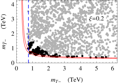
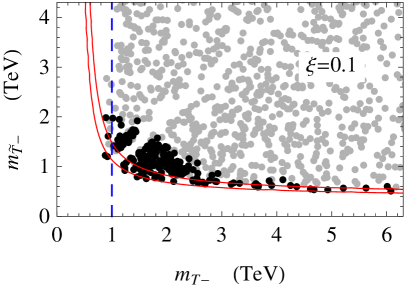
Figure 2: Scatter plots of the masses of the lightest $T$ and $\widetilde{T}$ resonances for $\xi=0.2$ (left panel) and $\xi=0.1$ (right panel) in the three-site DCHM model. The black dots denote the points for which $115\ {\rm GeV}\leq m_{H}\leq 130\ {\rm GeV}$, while the gray dots have $m_{H}>130\ {\rm GeV}$. The scans have been obtained by varying all the composite sector masses in the range $[-8f,8f]$ and keeping the top mass fixed at the value $m_{t}=150\ {\rm GeV}$. The area between the solid red lines represents the range obtained by applying the result in eq. (50) for $115\ {\rm GeV}\leq m_{H}\leq 130\ {\rm GeV}$. The dashed blue line corresponds to the estimate of the lower bound on $m_{T-}$ given in eq. (54).

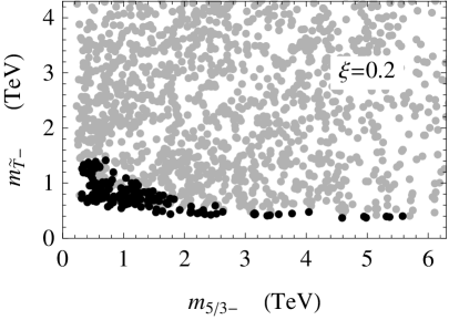
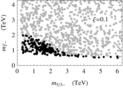
Figure 3: Scatter plots of the masses of the lightest exotic state of charge $5/3$ and of the lightest $\widetilde{T}$ resonance for $\xi=0.2$ (left panel) and $\xi=0.1$ (right panel) in the three-site DCHM model. The black dots denote the points for which $115\ {\rm GeV}\leq m_{H}\leq 130\ {\rm GeV}$, while the gray dots have $m_{H}>130\ {\rm GeV}$. The scans have been obtained by varying all the composite sector masses in the range $[-8f,8f]$ and keeping the top mass fixed at the value $m_{t}=150\ {\rm GeV}$.

We checked numerically the validity of our results by a scan on the parameter space of the model. In our numerical analysis we take the interval $115\ {\rm GeV}\leq m_{H}\leq 130\ {\rm GeV}$ as the range of Higgs masses compatible with the current LHC exclusion bounds. This range has been chosen slightly larger than the current exclusion for a SM-like Higgs to take into account the corrections due to the composite nature of the Higgs [24]. In our analysis we also fix the top mass to the value $m_{t}=m_{t}^{\overline{MS}}(2\ {\rm TeV})=150\ {\rm GeV}$, which corresponds to $m_{t}^{pole}=173\ {\rm GeV}$.

The scatter plots of the masses of the $T$ and $\widetilde{T}$ light resonances are shown in fig. 2. One can see that eq. (50) describes accurately the relation between the Higgs and the resonance masses in the regions in which one state is significantly lighter than the others. For a realistic Higgs mass this happens only when the $\widetilde{T}_{-}$ is much lighter than the other states. Instead, the situation of a $T$ much lighter than the $\widetilde{T}$ can not happen for a light Higgs due to the presence of a lower bound on the $m_{T_{-}}$, which will be discussed in details in the next section. In the region of comparable $T_{-}$ and $\widetilde{T}_{-}$ masses sizable deviations from eq. (50) can occur. These are due to the possible presence of a relatively light second level of resonances, as already discussed.

The numerical results clearly show that resonances with a mass of the order or below $1.5\ {\rm TeV}$ are needed in order to get a realistic Higgs mass both in the case $\xi=0.2$ and $\xi=0.1$. The prediction is even sharper for the cases in which only one state, namely the $\widetilde{T}_{-}$, is light. In these regions of the parameter space a light Higgs requires states with masses around $400\ {\rm GeV}$ for the $\xi=0.2$ case and around $600\ {\rm GeV}$ for $\xi=0.1$.

The situation becomes even more interesting if we also consider the masses of the other composite resonances. As we already discussed, the first level of resonances contains, in addition to the $T_{-}$ and $\widetilde{T}_{-}$, three other states: a top-like state, the $T_{2/3-}$, a bottom-like state, the $B_{-}$, and an exotic state with charge $5/3$, the $X_{5/3-}$. These three states together with the $T_{-}$ form a fourplet of SO(4). Obviously the $X_{5/3-}$ cannot mix with any other state even after EWSB, and therefore it remains always lighter than the other particles in the fourplet. In particular (see fig. 9 for a schematic picture of the spectrum), it is significantly lighter than the $T_{-}$ . In fig. 3 we show the scatter plots of the masses of the lightest exotic charge $5/3$ state and of the $\widetilde{T}$. In the parameter space region in which the Higgs is light the $X_{5/3-}$ resonance can be much lighter than the other resonances, especially in the configurations in which the $T_{-}$ and $\widetilde{T}_{-}$ have comparable masses. In these points the mass of the exotic state can be as low as $300\ {\rm GeV}$.

Notice that in the plots in fig. 2 there are no points in which the masses of the $T_{-}$ and of the $\widetilde{T}_{-}$ coincide. This is due to a repulsion of the mass levels induced by the mixings due to EWSB. As expected, this effect is more pronounced for larger values of $\xi$.

3.4 The top mass and a lower bound on the Higgs mass

As noticed above, the asymptotic region $m_{T-}\ll m_{\widetilde{T}-}$, which could in principle give rise to configurations with realistic Higgs masses, is not accessible in our model. Indeed in the scatter plots of fig. 2 we find a lower bound on $m_{T-}$. We will show below that this bound comes from the requirement of obtaining a realistic top mass and that an analogous bound, which however is not visible in fig. 2, exists for the $\widetilde{T}_{-}$ mass. From these results we will also derive an absolute lower bound on the Higgs mass.

The starting point of our analysis is the approximate expression for the top mass in eq. (47). Our aim is to abtain a lower bound on the resonance masses, so we will focus on the configurations in which one of the top partners is much lighter than the others. For definiteness we will consider the case in which the lightest state is the $T_{-}$ resonance. In a generic situation, all the parameters of the composite sector are of the same order $\Delta\sim m\sim\widetilde{m}_{Q}\sim\widetilde{m}_{T}$. The only mass which gets cancelled is $m_{T_{-}}$, so we can also assume that $m_{T_{+}}\sim m_{\widetilde{T}_{+}}$ and that they are of the same order of the composite sector masses. In this regime the effective compositeness angles in eq. (48) can be approximated as

$$\sin\varphi_{L}\sim 1\,,\qquad\sin\varphi_{R}\simeq\frac{y_{R}f}{m_{\widetilde{T}_{-}}}\,.$$ (51)

The first equation comes from the fact that we assumed the $T_{-}$ state to be nearly massless before the mixing with the elementary sector. This condition is equivalent to the relation $\Delta^{2}-m\,\widetilde{m}_{Q}=0$ (see eq. (80) of [8]).

The expression for the top mass in eq. (47) now becomes

$$m_{t}\simeq\frac{y_{R}f}{2\sqrt{2}}\sin\left(\frac{2v}{f_{\pi}}\right)\simeq y_{R}v\,,$$ (52)

and, by using the relation between $y_{L}$ and $y_{R}$ in eq (43), we get

$$y_{L}\simeq\sqrt{2}\,y_{R}\simeq\frac{\sqrt{2}m_{t}}{v}\,.$$ (53)

Given that the mass of the light state predominantly comes from the mixing with the elementary fermions we can use the estimate

$$m_{T_{-}}\gtrsim y_{L}f\simeq\frac{2m_{t}}{v}f_{\pi}\,.$$ (54)

This inequality implies the lower bounds

$$m_{T_{-}}\gtrsim 5m_{t}\simeq 750\ {\rm GeV}\,,\qquad{\rm for}\ \ \xi=0.2\,,$$ (55)

and

$$m_{T_{-}}\gtrsim 6.7m_{t}\simeq 1000\ {\rm GeV}\,,\qquad{\rm for}\ \ \xi=0.1\,,$$ (56)

obtained for $m_{t}=150\ {\rm GeV}$. In a similar way a lower bound on the mass of the lightest $\widetilde{T}$ state can be found. This bound is a factor $2$ weaker than the one on $m_{T-}$:

$$m_{\widetilde{T}_{-}}\gtrsim y_{R}f\simeq\frac{m_{t}}{v}f_{\pi}\,.$$ (57)

The lower bounds on the lightest top partners masses agree with the results of the numerical scans in fig. 2. The lower bound on $m_{\widetilde{T}_{-}}$ is instead below the range of values needed to get a realistic Higgs mass, so it is not visible in the the plot.

The lower bound on the resonance masses can be translated, through eq. (50) into a lower bound on the Higgs mass. The most favourable configuration is the one in which the lightest mass is $m_{\widetilde{T}_{-}}$. This leads to the bound

$$m_{H}\gtrsim\frac{\sqrt{2N_{c}}}{\pi}\frac{m_{t}^{2}}{v}\sqrt{\log\left(\frac{v}{m_{t}}\frac{m_{T_{-}}}{f_{\pi}}\right)}\,.$$ (58)

For $m_{T_{-}}/f_{\pi}\sim 4$, which represent a typical point in our parameter space, we get

$$m_{H}\gtrsim 100\ {\rm GeV}\,.$$ (59)

This result is in good agreement with the bound obtained in the scans.

4 The simplest composite Higgs model

As shown in Ref. [8], the three-site DCHM we considered in the previous section is the minimal realization of an effective description of a composite Higgs in which all the key observables, and in particular the Higgs potential, are computable at the leading order. This property allowed us to decouple the UV physics and fully characterize the model in terms of the parameters describing the elementary states and two levels of composite resonances.

Figure 4: Schematic structure of the two-site DCHM.

If we accept to give up a complete predictivity, a much simpler effective model can be employed to describe the low-energy dynamics of a composite Higgs boson and of the top partners. In this model only one layer of composite resonances is introduced, leading to a structure representable with a two-site model (see fig. 4). The pattern of divergences in the two-site DCHM has been fully analyzed in Ref. [8]: the electroweak precision parameters remain calculable at leading order, while the Higgs potential becomes logarithmically divergent at one loop.

There is however an interesting property which partially preserves predictivity also for the potential. In the expansion in powers of the elementary–composite mixings, only the leading terms can develop a logarithmic divergence, while the higher order ones are finite at one loop. We have shown in Section 2.1 (see eq. (20)) that at the leading order only two operators exist and that they both give the same contribution, proportional to $\sin^{2}{h/f_{\pi}}$, to the potential. A single counterterm is therefore enough to regulate the divergence, which corresponds to the renormalization of a single parameter. An interesting possibility is to fix the value of the Higgs VEV, or more precisely of the ratio $v/f_{\pi}$, as renormalization condition obtaining the Higgs mass as a prediction. In this sense, $m_{H}$ is predictable also in the DCHM₂.

4.1 Structure of the 2-site model

Let us briefly summarize the structure of the DCHM₂. The model is based on a non-linear $\sigma$-model ${\textrm{SO}}(5)_{L}\times{\textrm{SO}}(5)_{R}/{\textrm{SO}}(5)_{V}$ and it is schematically representation in fig. 4. As in the three-site DCHM, the first site is associated with the elementary states, while the other is related to the composite resonances. Of course, in this case, only one level of composite resonances is present. In order to accommodate the hypercharge for the fermions an extra ${\textrm{U}}(1)_{X}$ symmetry must be introduced, which acts on the fermion fields at both sites.

The elementary gauge bosons are added at the first site by gauging an $SU(2)_{L}\times{\textrm{U}}(1)_{Y}$ subgroup of ${\textrm{SO}}(5)_{L}\times{\textrm{U}}(1)_{X}$, with the choice of the hypercharge as $Y=T_{R}^{3}+X$. The composite gauge resonances are in the adjoint representation of ${\textrm{SO}}(4)$ and gauge a corresponding subgroup of ${\textrm{SO}}(5)_{R}$.

One level of composite fermions $\widetilde{\psi}$ is introduced at the second site. They transform in the fundamental representation of the ${\textrm{SO}}(5)_{R}$ global group and have ${\textrm{U}}(1)_{X}$ charge $2/3$. Analogously to the three-site case, the spontaneous breaking of ${\textrm{SO}}(5)$ in the composite sector is parametrized by the explicit breaking of the additional ${\textrm{SO}}(5)_{R}$ global group. In the fermionic sector this is achieved by a mass term which only respects the ${\textrm{SO}}(4)$ subgroup. The Lagrangian for the composite states $\widetilde{\psi}$, in the holographic gauge, is given by

$${\cal L}_{\textrm{comp}}^{\textrm{f}}=i\,\overline{\widetilde{\psi}}\hskip 3.0pt\raisebox{1.0pt}{$/$}D\widetilde{\psi}-\widetilde{m}_{\textrm{Q}}\overline{\widetilde{Q}}{\widetilde{Q}}-\widetilde{m}_{\textrm{T}}\overline{\widetilde{T}}\widetilde{T}\,,$$ (60)

where we have split $\widetilde{\psi}$ in ${\textrm{SO}}(4)$ representation, ${\bf 5}=({\bf 2},{\bf 2})\oplus({\bf 1},{\bf 1})$, as

$$\widetilde{\psi}=\left(\begin{array}[]{c}\widetilde{Q}\\ \widetilde{T}\end{array}\right)\,,$$ (61)

where $\widetilde{Q}\in({\bf 2},{\bf 2})$ and $\widetilde{T}$ is the singlet.

The elementary fermions, i.e. the SM chiral states $q_{L}$ and $t_{R}$, are introduced at the first site. Their Lagrangian is

$${\cal L}^{\textrm{f}}_{\textrm{elem}}=i\,\overline{q}_{L}\hskip 3.0pt\raisebox{1.0pt}{$/$}Dq_{L}+i\,\overline{t}_{R}\hskip 3.0pt\raisebox{1.0pt}{$/$}Dt_{R}-\,y_{L}f_{\pi}\overline{q}_{L}^{\bf 5}U\widetilde{\psi}_{R}-y_{R}\,f_{\pi}\overline{t}_{R}^{\bf 5}U\widetilde{\psi}_{L}+{\rm h.c.}\,,$$ (62)

where we used the embeddings of the elementary states in the fundamental representation of ${\textrm{SO}}(5)$ given in eq. (17).

Notice that we have already encountered the fermion Lagrangian of the DCHM₂ in the general discussion of section 2, and in particular at the end of section 2.1. The DCHM₂ can indeed be obtained from the general Lagrangian of eq. (28) by restricting $a_{L}=a_{R}=b_{L}=b_{R}$ in order to respect the ${\textrm{SO}}(5)$ symmetry.

4.2 The Higgs potential

Analogously to the DCHM₃ case, the fermionic contribution to the Higgs potential only comes from the charge $2/3$ states. Its structure can be put in the same form as eq. (38)

$$V(h)=-\frac{2N_{c}}{8\pi^{2}}\int dp\,p^{3}\log\left(1-\frac{C_{1}(p^{2})\sin^{2}(h/f_{\pi})+C_{2}(p^{2})\sin^{2}(h/f_{\pi})\cos^{2}(h/f_{\pi})}{D(p^{2})}\right)\,.$$ (63)

The denominator of the expression in the logarithm now contains only one level of resonances and is given by

$$D(p^{2})=2p^{2}\prod_{I=T,{\widetilde{T}},T_{2/3}}\big{(}p^{2}+m_{I}^{2}\big{)}\,,$$ (64)

where we used a notation similar to the one adopted for the three-site model. For the two-site model the expression for the masses of the top parteners before EWSB are very simple and can be given in closed form

$$m_{T}^{2}=\sqrt{\widetilde{m}_{Q}^{2}+(y_{L}f_{\pi})^{2}}\,,\qquad m_{T_{2/3}}^{2}=\widetilde{m}_{Q}^{2}\,,\qquad m_{\widetilde{T}}^{2}=\sqrt{\widetilde{m}_{T}^{2}+(y_{R}f_{\pi})^{2}}\,.$$ (65)

The $C_{1,2}$ coefficients appearing in the expression of the Higgs potential are given by

$$\left\{\begin{array}[]{l}C_{1}(p^{2})=-\left({\widetilde{m}}_{Q}^{2}-{\widetilde{m}}_{T}^{2}\right)p^{2}\left(\left(p^{2}+m_{T_{2/3}}^{2}\right)(y_{L}^{2}-2y_{R}^{2})f_{\pi}^{2}-y_{L}^{2}y_{R}^{2}f_{\pi}^{4}\right)\\ \rule{0.0pt}{15.00002pt}C_{2}(p^{2})=-({\widetilde{m}}_{Q}-{\widetilde{m}}_{T})^{2}\left(p^{2}+m_{T_{2/3}}^{2}\right)y_{L}^{2}y_{R}^{2}f_{\pi}^{4}\end{array}\right.\,.$$ (66)

Similarly to the three-site model, the second term appearing in the logarithm argument in eq. (63) is typically much smaller than one, so that we can use a series expansion. The potential, taking into account terms up to the quartic order in the elementary–composite mixings, has the usual form

$$V(h)\simeq\alpha\sin^{2}(h/f_{\pi})-\beta\sin^{2}(h/f_{\pi})\cos^{2}(h/f_{\pi})\,.$$ (67)

As we already mentioned, the ${\cal O}(y_{L,R}^{2})$ terms in the potential are logarithmically divergent, as can be easily checked using the explicit results given above. This implies that the coefficient $\alpha$ in eq. (67) must be regularized. For this purpose we can add a counterterm of the form given in eq. (20) with a suitable coefficient. This procedure is equivalent, from a practical point of view, to just consider $\alpha$ as a free parameter. This coefficient can then be fixed by imposing one renormalization condition, for instance by choosing the value of $v/f_{\pi}$.

Notice that, differently from the three-site model, in the two-site case there is no reason to assume that the leading order term in the potential is cancelled by a tuning among $y_{L}$ and $y_{R}$. The tuning of the potential can be totally due to the counterterm which cancels the logarithmic divergence. For this reason, in the following analysis we will not impose any relation between the left and the right elementary–composite mixings.

In order to compute the coefficient $\beta$ at quartic order in $y_{L,R}$ we need to take into account an expansion of the logarithm in eq. (63) at the quadratic order. The value of the coefficient $\beta$ can be easily found analytically and is given by

$$\beta = \frac{N_{c}}{8\pi^{2}}\frac{({\widetilde{m}}_{Q}-{\widetilde{m}}_{T})^{2}y_{L}^{2}y_{R}^{2}f_{\pi}^{4}}{m_{T}^{2}-m_{\widetilde{T}}^{2}}\log\left(\frac{m_{T}}{m_{\widetilde{T}}}\right)$$ (68)

$$+\frac{N_{c}}{8\pi^{2}}\frac{({\widetilde{m}}_{Q}^{2}-{\widetilde{m}}_{T}^{2})^{2}(y_{L}^{2}-2y_{R}^{2})^{2}f_{\pi}^{4}\left[-(m_{T}^{2}-m_{\widetilde{T}}^{2})+(m_{T}^{2}+m_{\widetilde{T}}^{2})\displaystyle\log\left(\frac{m_{T}}{m_{\widetilde{T}}}\right)\right]}{4(m_{T}^{2}-m_{\widetilde{T}}^{2})^{3}}\,.$$

The term on the first line of the above expression is analogous to the result found in the three-site case. On the other hand, the second contribution is specific of the two-site model and is there because we did not impose any relation between $y_{L}$ and $y_{R}$. The accidental factor of $4$ in the denominator of the second contribution and some cancellations which happen in the expression between square brackets make the second contribution smaller than the first one typically by one order of magnitude. Notice, moreover, that the sign of the two contributions are always the same. Thus the second contribution always determine a small increase of $\beta$ in absolute size. Neglecting this second term we obtain a Higgs mass

$$m_{H}^{2}=\frac{2\beta}{f_{\pi}^{2}}\sin^{2}(2v/f_{\pi})\simeq\frac{N_{c}}{4\pi^{2}}\frac{({\widetilde{m}}_{Q}-{\widetilde{m}}_{T})^{2}y_{L}^{2}y_{R}^{2}f_{\pi}^{2}}{m_{T}^{2}-m_{\widetilde{T}}^{2}}\log\left(\frac{m_{T}}{m_{\widetilde{T}}}\right)\sin^{2}(2v/f_{\pi})\,.$$ (69)

As we did in the three-site model, we can rewrite the Higgs mass in terms of the top mass. The approximate expression for the top mass was already found in section 2.1 (eq. (32)) and is given by

$$m_{t}\simeq\frac{|\widetilde{m}_{Q}-\widetilde{m}_{T}|}{2\sqrt{2}}\frac{y_{L}y_{R}f_{\pi}^{2}}{m_{T}m_{\widetilde{T}}}\sin\left(\frac{2v}{f_{\pi}}\right)\,.$$ (70)

Making use of eq. (69) we find

$$\frac{m_{H}}{m_{t}}\simeq\frac{\sqrt{2N_{c}}}{\pi}\frac{m_{T}m_{{\widetilde{T}}}}{f_{\pi}}\sqrt{\frac{\log\big{(}m_{T}/m_{{\widetilde{T}}}\big{)}}{m_{T}^{2}-m_{{\widetilde{T}}}^{2}}}\,,$$ (71)

which exactly coincides with the expression (50) obtained in the three-site model when the second level of resonances is heavy.

4.3 Numerical results

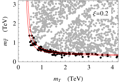
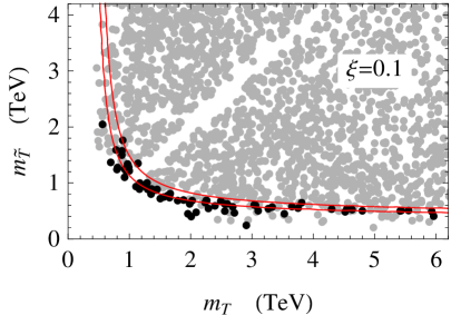
Figure 5: Scatter plots of the masses of the $T$ and $\widetilde{T}$ resonances for $\xi=0.2$ (left panel) and $\xi=0.1$ (right panel) in the two-site DCHM model. The black dots denote the points for which $115\ {\rm GeV}\leq m_{H}\leq 130\ {\rm GeV}$, while the gray dots have $m_{H}>130\ {\rm GeV}$. The scans have been obtained by varying all the composite sector masses in the range $[-8f_{\pi},8f_{\pi}]$ and keeping the top mass fixed at the value $m_{t}=150\ {\rm GeV}$. The area between the solid red lines represents the range obtained by applying the result in eq. (71) for $115\ {\rm GeV}\leq m_{H}\leq 130\ {\rm GeV}$.

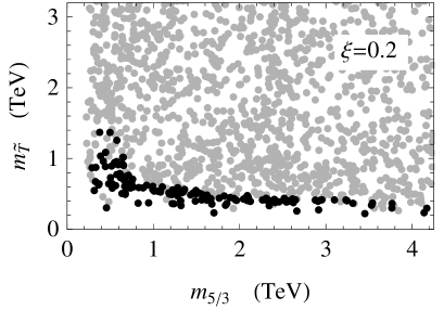
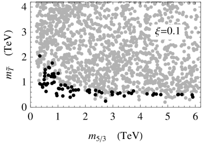
Figure 6: Scatter plots of the masses of the exotic state of charge $5/3$ and of the $\widetilde{T}$ resonance for $\xi=0.2$ (left panel) and $\xi=0.1$ (right panel) in the two-site DCHM model. The black dots denote the points for which $115\ {\rm GeV}\leq m_{H}\leq 130\ {\rm GeV}$, while the gray dots have $m_{H}>130\ {\rm GeV}$. The scans have been obtained by varying all the composite sector masses in the range $[-8f_{\pi},8f_{\pi}]$ and keeping the top mass fixed at the value $m_{t}=150\ {\rm GeV}$.

We can verify the validity of the relation in eq. (71) between the Higgs and the top partners masses by performing a numerical scan on the parameter space of the two-site model. However the computation of the Higgs effective potential in the two-site case is not completely straightforward and requires an ad hoc procedure to deal with the logarithmic divergence. In particular, we can not directly integrate eq. (63) as in the $3$-site model. The simplest way to proceed is to notice that eq. (63) can be rewriten in the standard Coleman–Weinberg form

$$V(h)=-\frac{2N_{c}}{8\pi^{2}}\int dp\ p^{3}\log\left[\prod_{i}(p^{2}+m_{i}^{2}(h))\right]\,,$$ (72)

where the product is over all the $2/3$-charged fermionic states of our model. Actually, we could have derived eq. (63) starting from the Coleman–Weinberg expression in eq. (72). We can now regulate the integral with a hard momentum cutoff $\Lambda$ and we obtain the standard formula

$$V(h)=-\frac{N_{c}}{8\pi^{2}}\Lambda^{2}\sum_{i}m_{i}^{2}(h)-\frac{N_{c}}{16\pi^{2}}\sum_{i}m_{i}^{4}(h)\left[\log\left(\frac{m_{i}^{2}(h)}{\Lambda^{2}}\right)-\frac{1}{2}\right]\,.$$ (73)

In the two-site model only a logarithmic divergence can appear in the Higgs potential, and therefore the quadratically divergent term must be independent of the Higgs. This is ensured by the condition

$$\sum_{i}m_{i}^{2}(h)=\sum_{i}m_{i}^{2}(h=0)={\rm const}.\,,$$ (74)

which we can explicitly verify in our model. The logarithmic divergence, as discussed above, must be proportional to $\sin^{2}{h/f_{\pi}}$ as in eq. (20). Indeed in our $2$-site model one can verify explicitly that

$$\sum_{i}m_{i}^{4}(h)\propto\sin(h/f_{\pi}^{2})+{\rm const}\,.$$

We can therefore, as anticipated, cancel the divergence by introducing a single counterterm in the potential, proportional to $\sin^{2}{h/f_{\pi}}$. This leaves only one free renormalization parameter which we can trade for a scale $\mu$, the renormalized potential takes the form

$$V(h)=-\frac{N_{c}}{16\pi^{2}}\sum_{i}m_{i}^{4}(h)\log\left(\frac{m_{i}^{2}(h)}{\mu^{2}}\right)\,.$$ (75)

We will treat $\mu$ as a free parameter, the strategy of our scan will be to choose it, once the other parameters are fixed, in order to fix the minimum of the potential to the required value of $v/f_{\pi}$.

The result of the numerical scan is shown in fig. 5. The black points correspond to configuration with realistic Higgs mass and they lie approximately between the two solid red lines which correspond to the bounds derived from eq. (71). The small deviations come from the corrections due to the $(y_{L}^{2}-2y_{R}^{2})$ term in the expression for $\beta$ in eq. (68). As discussed before, the effect of these corrections is to increase the Higgs mass, and therefore, keeping the Higgs mass fixed, to make the resonances lighter. In fig. 5 we show the scatter plot of masses of the exotic charge $5/3$ state and of the $\widetilde{T}$. As in the three-site model the exotic state is lighter than the $T$, so that, in a large part of the parameter space it is the lightest composite resonance.

4.4 Modeling the effect of the heavy resonances

By comparing the scatter plots obtained for the two-site model with the ones for the three-site one, one can see that, although the relation between the Higgs mass and the resonance masses is always reasonably well satisfied, significant deviations can appear. In particular the region in which $m_{T}$ and $m_{\widetilde{T}}$ are comparable shows larger deviations, while the asympthotic regions in which one of the resonances is much lighter than the others have a smaller spread. The $2$-site model is therefore slightly too restrictive, and also too “pessimistic” in that it requires very low resonances. The effect of an additional level of resonances, as the $3$-site model results show, can change the $2$-site picture significantly.

However, the effect of the heavy resonances on the Higgs potential can be rather simply mimicked in the two-site model by adding to the potential a new contribution to the coefficient $\beta$ in eq. (67). The size of the contributions coming from the heavy resonances can be estimated by symmetry considerations and power counting. In our derivation we will respect the general properties which characterize the heavy resonances in the three-site model. First of all we assume that the source of ${\textrm{SO}}(5)$ breaking is in common with the light states, so that the new operator must contain a factor $({\widetilde{m}}_{Q}-{\widetilde{m}}_{T})^{2}$. Morever we must introduce four powers of the elementary–composite mixings as dictated by spurion analysis. For simplicity we will write the contribution of the new operator to $\beta$ in the same form of the contribution coming from the light states. In particular we choose the form of the most relevant term, the one on the first line of eq. (68). Denoting by $M$ the mass of the heavy resonances we write their contribution to the Higgs effective potential as

$$\Delta V(h)=\frac{N_{c}}{8\pi^{2}}\frac{({\widetilde{m}}_{Q}-{\widetilde{m}}_{T})^{2}y_{L}^{2}y_{R}^{2}f_{\pi}^{4}}{M^{2}}\sin^{2}(v/f_{\pi})\cos^{2}(v/f_{\pi})\,.$$ (76)

Guided by the results of the three-site model, in which the heavy resonances tend to lower the Higgs mass, we fix the sign for the corrections in order to reproduce this effect.

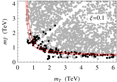
Figure 7: Scatter plots of the masses of the $T$ and $\widetilde{T}$ resonances for $\xi=0.2$ (left panel) and $\xi=0.1$ (right panel) in the two-site DCHM model with the addition of the operator in eq. (76). The black dots denote the points for which $115\ {\rm GeV}\leq m_{H}\leq 130\ {\rm GeV}$, while the gray dots have $m_{H}>130\ {\rm GeV}$. The scans have been obtained by varying all the composite sector masses in the range $[-8f_{\pi},8f_{\pi}]$ and keeping the top mass fixed at the value $m_{t}=150\ {\rm GeV}$. The mass of the heavy resonances has been chosen to be at least $50\%$ higher than the one of all the light states. The area between the solid red lines represents the range obtained by applying the result in eq. (71) for $115\ {\rm GeV}\leq m_{H}\leq 130\ {\rm GeV}$.

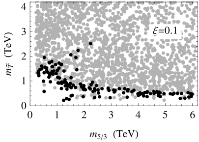
Figure 8: Scatter plots of the masses of the exotic state of charge $5/3$ and of the $\widetilde{T}$ resonance for $\xi=0.2$ (left panel) and $\xi=0.1$ (right panel) in the two-site DCHM model with the addition of the operator in eq. (76). The black dots denote the points for which $115\ {\rm GeV}\leq m_{H}\leq 130\ {\rm GeV}$, while the gray dots have $m_{H}>130\ {\rm GeV}$. The scans have been obtained by varying all the composite sector masses in the range $[-8f_{\pi},8f_{\pi}]$ and keeping the top mass fixed at the value $m_{t}=150\ {\rm GeV}$. The mass of the heavy resonances has been chosen to be at least $50\%$ higher than the one of all the light states.

The numerical results of a scan including the effect of the operator in eq. (76) are shown in fig. 7. In the scan we assume that the mass of the heavy resonances is at least $50\%$ higher than the masses of all the light resonances. One can see that the plots show a good qualitative and quantitative agreement with the ones obtained in the three-site model (see fig. 2). In particular the plots show an agreement with the relation in eq. (71) in the asymptotic regions in which one state is much lighter than the others. Larger deviations are present when all the state have comparable masses. This effect can be simply understood by comparing the form of the leading contributions to $\beta$ in eq. (68) (the ones on the first line) and the form of the contributions of the operator representing the heavy resonances in eq. (76). When a high hierarchy between $m_{T}$ and $m_{\widetilde{T}}$ is present, the logarithm appearing in eq. (68) enhances the light states contributions to the Higgs mass, thus making the heavy resonances corrections negligible. On the other hand, when $m_{T}\sim m_{\widetilde{T}}$, the light states contribution are somewhat reduced and the heavy states can give a sizable correction to $\beta$.

Finally in fig. 8 we show the scatter plot for the masses of the exotic charge $5/3$ state and of the ${\widetilde{T}}$ state. Again a good agreement with the results for the three-site model in fig. 3 is found.

5 Bounds on the top partners

The top partners are generically so light, often below the TeV, than the present experimental results can already place some non-trivial bounds on their mass. In this section we will present a simple discussion of the available constraints; our aim will not be to perform a comprehensive study of all the bound coming from the existing experimental data, but instead to focus on some simple and universal searches whose results are approximately valid independently of the specific model and of the corner of the parameter space we consider.

In particular we will restrict our analysis to the lightest resonance which comes from the composite sector and we will only consider pair production processes in which, due to the universal QCD couplings, the production cross section depends exclusively on the mass of the resonance. The bounds we will derive are thus quite robust and apply to generic composite models. Notice however that, in a large region of the parameter space, single production processes, as well as the presence of other relatively light resonances, can give an enhancement of the signal in the channels considered in the present analysis. In this case the bounds on the masses of the resonances can also become tighter. Taking into account these effects is however beyond the scope of the present paper.

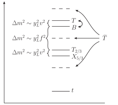
Figure 9: Schematic structure of the spectrum of the lightest multiplet of resonances.

Before discussing the details of our analysis, it is useful to briefly describe the general structure of the spectrum of the first level of fermionic resonances. These states, as schematically shown in fig. 9, are approximately organized in $SU(2)_{L}$ multiplets

$$Q=\left(\begin{array}[]{cc}T\\ B\end{array}\right)\,,\qquad X=\left(\begin{array}[]{cc}X_{5/3}\\ T_{2/3}\end{array}\right)\,,\qquad\widetilde{T}\,.$$ (77)

The splitting between the two doublets arises from the mixing of the composite fermions with the elementary states and its size is of order $\Delta m^{2}\sim y_{L}^{2}f^{2}$. Notice that only the $Q$ doublet is mixed to the elementary fermions, thus it is always heavier than the $X$ doublet. On the other hand, the mass of the $\widetilde{T}$ singlet has no relation to the ones of the two doublets.

After the breaking of the electroweak symmetry the fermions acquire mass corrections giving rise to a small splitting inside the doublets. Due to the Goldstone nature of the Higgs, the effects of EWSB can only arise if the Goldstone symmetry is broken, that is they must be mediated by the elementary–composite mixings. The mass splitting inside the doublets are thus of order $y_{L,R}^{2}v^{2}$, and are typically suppressed by a factor $(v/f)^{2}$ with respect to the mass gap between the two doublets. For all the relevant configurations the lightest state of the $X$ doublet is the exotic fermion with charge $5/3$, the $X_{5/3}$. The ordering of the states in the $Q$ multiplet instead is not fixed and depends on the specific point in the parameter space we choose.

As we mentioned before, in our analysis we will only consider the lightest fermionic resonance, which is always given by the exotic state $X_{5/3}$ or by the singlet $\widetilde{T}$. We will discuss these two cases separately in the following subsections.

5.1 Bounds on the exotic charge $5/3$ state

As a first case we will consider the configurations in which the exotic state $X_{5/3}$ is the lightest new resonance. A search for an exotic state of this type has been performed by the CDF collaboration [25]. This analysis focuses on the case in which the exotic state is associate with a charge $-1/3$ fermion, the $B$, with the same mass. Moreover it is assumed that these two states always decay in $tW^{\pm}$. The considered channel is pair production of the new resonances, which then give rise to a signal in events with two same-sign leptons. With an integrated luminosity of $2.7\ {\rm fb}^{-1}$, masses of the new states $m_{5/3}=m_{B}<365\ {\rm GeV}$ are excluded at $95\%$ confidence level.

Dedicated searches for charge $5/3$ states are currently not available for the LHC data. Some interesting bounds on the mass of the exotic states can however be derived by adapting the existing searches of new bottom-like resonances. The analyses we can use for our aim are the ones in which the bottom-like resonance $B$ is pair produced and decays in top: $B\overline{B}\rightarrow W^{-}tW^{+}\overline{t}$. The same final state is obviously obtained also in a process in which a pair of exotic states $X_{5/3}$ are produced, which then decay to SM particles: $X_{5/3}\overline{X}_{5/3}\rightarrow W^{+}tW^{-}\overline{t}$.

The strongest exclusion bound on new bottom-like quarks decaying in tops is the one obtained by the CMS Collaboration [18], which sets a lower bound $m_{B}>611\ {\rm GeV}$ at $95\%$ confidence level assuming $BR(B\rightarrow W^{-}t)=1$. This analysis is performed by condidering final states with a pair of same-sign leptons or with three leptons. To translate this result into an exclusion bound for the exotic $X_{5/3}$ resonance, we need to take into account possible differences in the efficiencies for the cuts used in the analysis. These differences can arise from finite-width effects and from the different kinematic distribution of the final states of the two processes. In particular in the $X_{5/3}\overline{X}_{5/3}$ process the two same-sign leptons come from the decay of the same heavy particle, while in the $B\overline{B}$ case they come from different heavy legs. The structure of the cuts used in the analysis, however, is rather symmetric with respect to the leptons, so we expect the efficiencies to be reasonably close. To determine the variation of the cut acceptances we simulated the signal using our implementation of the three- and two-site models in MadGraph 5. We found that the deviations from the $B\overline{B}$ process are always negligible (below $5\%$).

The production cross sections for $X_{5/3}\overline{X}_{5/3}$ and $B\overline{B}$ are equal, given that the two processes are induced by QCD. Moreover, being the $X_{5/3}$ the lightest resonance, it can only decay to the SM, so that $BR(X_{5/3}\rightarrow W^{+}t)=1$. This means that we can directly reinterpret the exclusion bound on the bottom-like resonances as a lower bound on the mass of the exotic state $X_{5/3}$: $m_{5/3}>611\ {\rm GeV}$.

Notice that the presence of other resonances with a mass relatively close to the $X_{5/3}$, and in particular a light $B$, can sizably enhance the signal used in the previous analysis, thus leading to stronger bounds. The analysis of this effect is however beyond the scope of the present paper.

5.2 Bounds on the $\widetilde{T}$

We now focus on the case in which the lightest resonance is given by the charge $2/3$ state $\widetilde{T}$. For a state of this kind exclusion analysis have been performed for the available LHC data. At present the strongest bounds are the ones obtained by the CMS Collaboration. They considered two possible scenarios in which a top-like resonance decays with $100\%$ branching ratio either in $tZ$, yielding a bound $m_{t^{\prime}}>475\ {\rm GeV}$ [28], or in $bW^{+}$, with bounds $m_{t^{\prime}}>560\ {\rm GeV}$ [29] and $m_{t^{\prime}}>552\ {\rm GeV}$ [30] depending on the specific final states considered.

These bounds can not be directly translated into bounds on the $\widetilde{T}$ resonance in our model, due to the different branching ratios of the resonance into SM particles. In particular three channels are relevant $\widetilde{T}\rightarrow bW^{+}$, $\widetilde{T}\rightarrow tZ$ and $\widetilde{T}\rightarrow th$. The branching ratios for these three channels are all comparable, hence a process in which two $\widetilde{T}$ resonances are produced, which then decay in the same channel, has a cross section which is usually an order of magnitude smaller than the total pair production cross section. From a scan on the parameter space of the explicit models, see fig. 10, we find that typically the $W$ and Higgs channels dominate, $BR(\widetilde{T}\rightarrow bW^{+})\sim BR(\widetilde{T}\rightarrow th)\sim 0.4$, while the $Z$ channel is slightly suppressed, $BR(\widetilde{T}\rightarrow tZ)\sim 0.2$.

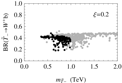
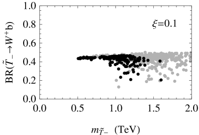
Figure 10: Scatter plot of the branching ratios of the lightest $\widetilde{T}$ resonance into $W^{+}b$ for the three-site DCHM model with $\xi=0.2$ (left panel) and $\xi=0.1$ (right panel). In all the points shown in the plot the $\widetilde{T}$ state has been required to be the lightest composite resonance. The black dots denote the points for which $115\ {\rm GeV}\leq m_{H}\leq 130\ {\rm GeV}$, while the gray dots have $m_{H}>130\ {\rm GeV}$. The scans have been obtained by varying all the composite sector masses in the range $[-8f,8f]$ ane keeping the top mass fixed to the value $m_{t}=150\ {\rm GeV}$.

To find an exclusion bound on the $\widetilde{T}$ resonance we adopt the simple and conservative approach of just rescaling the cross section of each channel considered in the experimental analysis by the typical branching ratios predicted by our models for a low resonance mass. Of course, a more refined procedure, would need to take into account possible enhancements of the signal coming from the other decay channels. For instance, in the search of a top-like resonance decaying in $Zt$ [28] the masses of the resonances are not reconstructed and only a mild cut is put to reconstruct one of the $Z$’s. In this case a sizable part of events in which one or even both $\widetilde{T}$ resonances do not decay in $Zt$ could pass the selection cuts and significantly enhance the signal, thus tightening the exclusion bounds.

Following our simple approach we find that only one of the searches gives a significant bound, namely the one exploiting the channel $\widetilde{T}\overline{\widetilde{T}}\rightarrow bW^{+}\overline{b}W^{-}\rightarrow bl^{+}\nu\overline{b}l^{-}\overline{\nu}$ [30]. To obtain the bound we performed the analysis using for the relevant branching ratio the value $BR(\widetilde{T}\rightarrow bW^{+})=0.4$. As can be seen by the scatter plot in fig. 10, this value represents the actual branching ratio for a light $\widetilde{T}$ in the three-site DCHM model, quite independently of the value of $v/f_{\pi}$. With this procedure we infer a lower bound $m_{\widetilde{T}}>370\ {\rm GeV}$ on the mass of the $\widetilde{T}$ resonance at $95\%$ confidence level.

5.3 Exclusion bounds in the DCHM₃

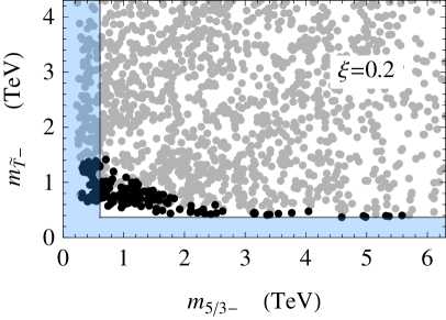
Figure 11: Scatter plot of the masses of the lightest exotic state of charge $5/3$ and of the lightest $\widetilde{T}$ resonance for the three-site DCHM model with $\xi=0.2$ (left panel) and $\xi=0.1$ (right panel). The shaded region corresponds to the points excluded by our analysis, which gives the bounds $m_{5/3}>611\ {\rm GeV}$ and $m_{\widetilde{T}}>370\ {\rm GeV}$. The black dots denote the points for which $115\ {\rm GeV}\leq m_{H}\leq 130\ {\rm GeV}$, while the gray dots have $m_{H}>130\ {\rm GeV}$.

To appreciate the impact of the previously derived bounds in the explicit models we show in fig. 11 the exclusion regions superimposed on the scatter plots for the masses of the $X_{5/3}$ and $\widetilde{T}$ resonances for the three-site DCHM model.

The bound on the exotic state with chagre $5/3$ is already strong enough to exclude a sizable portion of the parameter space with realistic Higgs mass. Of course, the bound has a greater impact on the configurations with larger $\xi$, which predict lighter resonances. Nevertheless even in the case of a relatively small $v/f_{\pi}$, namely $\xi=0.1$, the exclusion bound on the exotic resonance puts non-trivial constraints.

The situation is different for the cases in which the lightest new state is the singlet $\widetilde{T}$. The bounds obtained in our analysis can only exlude a limited number of configurations at $\xi$ relatively large. In particular for $\xi=0.2$ realistic configurations start to be excluded only in the asymptotic region with a light $\widetilde{T}$. On the other hand, for $\xi=0.1$ the mass of the $\widetilde{T}$ resonances is always above the current bounds.

6 Conclusions and outlook

In this paper we explored the relation which, in a broad class of composite Higgs models, links a light Higgs boson to the presence of light resonances coming from the new strong sector of the theory. The class of models we focused on are the ones based on the symmetry pattern SO(5)/SO(4) and in which the fermionic resonances come in the fundamental representation of SO(5). As a first step, we analyzed from a general point of view the mechanism which generates the correlation of the Higgs mass with the top partners. We found that the connection has a simple qualitative explanation in terms of the structure of partial fermion compositeness which is realized in the composite Higgs scenario. The point is that the presence of light partners would tend to increase the fraction of top quark compositeness, thus increasing its mass. Keeping the latter fixed requires that the elementary–composite mixings, must be decreased in order to compensate. But the mixings also control the Higgs potential, and their decrease lowers the the Higgs quartic coupling and consequently the Higgs mass.

Through a detailed analysis performed in a general effective parametrization of the composite Higgs set-up, we found that the Higgs mass scales linearly with the mass of the lightest partner. This model-independent result is encoded in the simple relation of eq. (31). The relevant partners are those which are most strongly mixed with the elementary $t_{L}$ and $t_{R}$, namely the $T$ and the $\widetilde{T}$ resonances.

From a quantitative point of view, assuming only a moderate degree of tuning between the Higgs VEV and the Goldstone decay constant $f_{\pi}$, we found that a Higgs mass in the current LHC preferred region $m_{h}\simeq 120\ {\rm GeV}$ requires at least one top partner with a mass of the order or below the ${\rm TeV}$. This result strengthens the common assertion that light top partners are an essential feature of the composite Higgs scenario. Moreover it shows that the lightest of such states are well within the reach of the LHC and they constitute one of the most important probes of the composite Higgs paradigm.

To confirm the validity of our general results we analyzed in detail the relation between the Higgs and the resonance masses in two explicit models. The first model we considered is the three-site Discrete Composite Higgs Model, which gives a simple but complete realization of the composite Higgs framework. Good agreement with the general result is found (see eq. (50)). The study of this explicit model allowed us to quantify the effects of the higher levels of resonances coming from the composite sector. Their contribution has been determined analytically (see eq. (44)) and checked numerically by a scan on the parameter space of the model (see figs. 2 and 3). We found that in the asymptotic regions in which there is a large mass hierarchy between the resonances of the first level, the effect of the heavier states is very small. On the contrary, when the masses are comparable the corrections can be sizable and can affect the Higgs mass by as much as $50\%$. These corrections, however, do not spoil the agreement with the qualitative picture obtained by the general analysis.

As a second explicit model, we considered an even simpler and more minimal implementation of the composite Higgs idea, the two-site Discrete Composite Higgs Model. This model contains only one level of composite resonances, thus it only retains the amount of information relevant for the present collider experiments. The price we have to pay in adopting this minimal description is a partial loss of predictivity: in the two-site model the Higgs potential is no more finite at one loop. Nevertheless only one counterterm is needed to regulate the divergence, thus one condition is enough to fix the renormalization ambiguity. We can therefore chose the value of $v/f_{\pi}$ as a renormalization condition and retain the Higgs mass as a calculable quantity.

We also showed how the effect of the higher resonance levels on the Higgs potential can be efficiently modeled by introducing a suitable extra contribution. With this modification, the spectrum of the top partners in correlation with the Higgs mass is completely analogous to the one found in the three-site case.

Generically, our result should apply to any explicit realization of the composite Higgs idea, and in particular to the popular 5d holographic models. This is partially confirmed by the numerical results of Ref. [5], which indeed show an approximately linear correlation between the mass of the Higgs and the one of the lightest $T$ state. From what can be seen in the plots, moreover, the agreement with our general formula seems good also at a quantitative level. It might be worth checking the agreement in more detail.

Another aspect which could be worth investigating is how much our results depend on the choice of the fermion representations. In the set-ups considered so far in the literature, in which the fermions are in the spinorial or in the adjoint representation of SO(5) there will be no qualitative difference with respect to the case of the fundamental we have considered in the present paper. The general analysis of section 2 will apply in the same way because also in these alternative scenarios only one invariant operator contributes to the Higgs potential at the leading order in the elementary–composite mixing. This implies that the leading order must be canceled and the Higgs mass squared scales as $y^{4}$ (rather than $y^{2}$) like in eq. (26). Also the estimate of the top mass will remain the same and therefore the final result of eq. (31) will be parametrically unchanged. At the quantitative level, however, the relation among the Higgs and the resonance masses could be modified at order one, due to possibly different group theory factors. It would be interesting to assess this point.

With other choices of the fermion representations, in which two or more invariants appear at order $y^{2}$, our conclusions could instead change qualitatively. A model of this kind could for instance be obtained by embedding the fermions in the adjoint but relaxing the requirement of left–right symmetry, or by considering higher and possibly reducible representations.

The models with more invariants are particularly interesting because they do not suffer of the enhanced (or “double”) tuning which we described in section 2 (see eq. (25)). This indeed originates only in the case of a single invariant because of the “preliminary” cancellation of the ${\cal O}(y^{2})$ term which is needed to make it of the same order of the subleading ${\cal O}(y^{4})$ contributions. Models in which the double tuning is not present, however, should face another possible problem. Given that the potential, including the quartic Higgs coupling, now arises at ${\cal O}(y^{2})$, the mass of the Higgs is expected to be a factor $g_{*}/y$ larger than in the models with the preliminary cancellation. The situation would therefore be worse than the one considered in the present paper, so we expect that either we will find a too large Higgs mass or too light top partners.

The last step of our work has been to derive some non trivial constraints on the resonance masses from the current LHC data. We performed a simple analysis in which only the lightest resonances have been considered and the contributions from heavier states have been altogether neglected. The lightest composite states are either the exotic partner of charge $5/3$, the $X_{5/3}$, or the SO(4) singlet top-like state $\widetilde{T}$. No dedicated LHC analysis exists for states of charge $5/3$, however the existing searches for pair-produced new bottom-like quarks can be used to derive some exclusion bounds also for the exotic resonance. Our simulations show that the current exclusion can be translated into a bound $m_{5/3}>611\ {\rm GeV}$. This bound is already enough to exclude a non-negligible portion of the configurations with a realistic Higgs mass.

The situation is different for the cases in which the lightest state is the $\widetilde{T}$. LHC searches for pair-produced charge $2/3$ resonances are available, however the bounds given in the experimental analyses can not be naively applied to the composite models, due to the fact that $100\%$ branching ratios to specific channels are assumed. Taking into account the branching ratios predicted by our explicit models, a lower bound $m_{\widetilde{T}}>370\ {\rm GeV}$ is obtained. This bound is still too weak to put significant constraints on the model. However it is not far from the masses obtained in realistic configurations and can already exclude a small region of the parameter space in the case $\xi=0.2$.

The simple analysis we used to derive the exclusion bounds leads to some robust and conservative constraints on the masses of the composite resonances. The assumption of having only one relevant light state and to consider only pair production is however a drastic simplification which often neglects important contributions. In particular some of the heavier states can be close enough to the lightest resonance to give a sizable contribution to the relevant search channels. Moreover single production processes can be relevant in specific regions of the parameter space. It is plausible that the inclusion of these effects could considerably strengthen the bounds we derived in this paper.

A complete study of the exclusion bound, including the effects of the heavier resonances and of single production, is not completely straightforward. An analysis of this kind should take into account possible decay chains from the heavier resonances as well as non-universal production cross sections due to single production channels. To perform this task it seems unavoidable to employ a concrete model. We already produced complete MadGraph 5 cards implementing the two-site and the three-site models. In particular the two-site model contains only three free parameters and one could imagine performing a complete scan. These cards were used in the present paper to adapt the experimental analysis and derive the bounds on the exotic state $X_{5/3}$. We leave for future work the complete study of the constraints coming from the experimental data.

References

- [1] G. Aad et al. [ATLAS Collaboration], Phys. Lett. B 710 (2012) 49 [arXiv:1202.1408 [hep-ex]].
- [2] S. Chatrchyan et al. [CMS Collaboration], arXiv:1202.1488 [hep-ex].
- [3] S. Dimopoulos, J. Preskill, Nucl. Phys. B199 (1982) 206. D. B. Kaplan, H. Georgi, Phys. Lett. B136 (1984) 183. D. B. Kaplan, H. Georgi, S. Dimopoulos, Phys. Lett. B136 (1984) 187. H. Georgi, D. B. Kaplan, P. Galison, Phys. Lett. B143 (1984) 152. T. Banks, Nucl. Phys. B243 (1984) 125. H. Georgi, D. B. Kaplan, Phys. Lett. B145 (1984) 216. M. J. Dugan, H. Georgi, D. B. Kaplan, Nucl. Phys. B254 (1985) 299.
- [4] K. Agashe, R. Contino, A. Pomarol, Nucl. Phys. B719 (2005) 165-187. [hep-ph/0412089].
- [5] R. Contino, L. Da Rold and A. Pomarol, Phys. Rev. D 75, 055014 (2007) [hep-ph/0612048].
- [6] R. Contino, T. Kramer, M. Son, R. Sundrum, JHEP 0705 (2007) 074. [hep-ph/0612180].
- [7] G. F. Giudice, C. Grojean, A. Pomarol, R. Rattazzi, JHEP 0706 (2007) 045. [hep-ph/0703164].
- [8] G. Panico, A. Wulzer, JHEP 1109 (2011) 135. [arXiv:1106.2719 [hep-ph]].
- [9] R. Barbieri, B. Bellazzini, V. S. Rychkov and A. Varagnolo, Phys. Rev. D 76 (2007) 115008 [arXiv:0706.0432 [hep-ph]].
- [10] R. Contino, Y. Nomura, A. Pomarol, Nucl. Phys. B671 (2003) 148-174. [hep-ph/0306259]. Y. Hosotani, M. Mabe, Phys. Lett. B615 (2005) 257-265. [hep-ph/0503020]. Y. Hosotani, S. Noda, Y. Sakamura, S. Shimasaki, Phys. Rev. D73 (2006) 096006. [hep-ph/0601241]. M. S. Carena, E. Ponton, J. Santiago, C. E. M. Wagner, Nucl. Phys. B759 (2006) 202-227. [hep-ph/0607106]; Phys. Rev. D76 (2007) 035006. [hep-ph/0701055]. A. D. Medina, N. R. Shah, C. E. M. Wagner, Phys. Rev. D76 (2007) 095010. [arXiv:0706.1281 [hep-ph]].
- [11] L. J. Hall, Y. Nomura, D. Tucker-Smith, Nucl. Phys. B639 (2002) 307-330. [hep-ph/0107331]. M. Kubo, C. S. Lim, H. Yamashita, Mod. Phys. Lett. A17 (2002) 2249-2264. [hep-ph/0111327]. G. Burdman, Y. Nomura, Nucl. Phys. B656 (2003) 3-22. [hep-ph/0210257]. N. Haba, M. Harada, Y. Hosotani, Y. Kawamura, Nucl. Phys. B657 (2003) 169-213. [hep-ph/0212035]. I. Gogoladze, Y. Mimura, S. Nandi, Phys. Lett. B560 (2003) 204-213. [hep-ph/0301014]; Phys. Rev. D69 (2004) 075006. [hep-ph/0311127]. C. A. Scrucca, M. Serone, L. Silvestrini, Nucl. Phys. B669 (2003) 128-158. [hep-ph/0304220]. G. Cacciapaglia, C. Csaki, S. C. Park, JHEP 0603 (2006) 099. [hep-ph/0510366]. G. Panico, M. Serone, A. Wulzer, Nucl. Phys. B739 (2006) 186-207. [hep-ph/0510373]; M. Sakamoto, K. Takenaga, Phys. Rev. D75 (2007) 045015. [hep-th/0609067]. C. S. Lim, N. Maru, Phys. Lett. B653 (2007) 320-324. [arXiv:0706.1397 [hep-ph]]. G. Panico, M. Safari, M. Serone, JHEP 1102 (2011) 103. [arXiv:1012.2875 [hep-ph]].
- [12] Nucl. Phys. B762 (2007) 189-211. [hep-ph/0605292]. G. Panico, E. Ponton, J. Santiago, M. Serone, Phys. Rev. D77 (2008) 115012. [arXiv:0801.1645 [hep-ph]].
- [13] D. B. Kaplan, Nucl. Phys. B365 (1991) 259-278.
- [14] R. Contino and G. Servant, JHEP 0806 (2008) 026 [arXiv:0801.1679 [hep-ph]]. J. A. Aguilar-Saavedra, JHEP 0911 (2009) 030 [arXiv:0907.3155 [hep-ph]]. J. Mrazek and A. Wulzer, Phys. Rev. D 81 (2010) 075006 [arXiv:0909.3977 [hep-ph]]. G. Dissertori, E. Furlan, F. Moortgat and P. Nef, JHEP 1009 (2010) 019 [arXiv:1005.4414 [hep-ph]].
- [15] N. Arkani-Hamed, A. G. Cohen and H. Georgi, Phys. Rev. Lett. 86 (2001) 4757 [hep-th/0104005]; C. T. Hill, S. Pokorski and J. Wang, Phys. Rev. D 64 (2001) 105005 [hep-th/0104035].
- [16] S. De Curtis, M. Redi and A. Tesi, JHEP 1204 (2012) 042 [arXiv:1110.1613 [hep-ph]].
- [17] H.-C. Cheng, J. Thaler, L.-T. Wang, JHEP 0609 (2006) 003. [hep-ph/0607205]. R. Foadi, J. T. Laverty, C. R. Schmidt, J.-H. Yu, JHEP 1006 (2010) 026. [arXiv:1001.0584 [hep-ph]]. M. Baumgart, [arXiv:0706.1380 [hep-ph]].
- [18] The CMS Collaboration, “Search for heavy bottom-like quarks in 4.9 inverse femtobarns of pp collisions at sqrt(s) = 7 TeV”, arXiv:1204.1088 [hep-ex].
- [19] J. Alwall, M. Herquet, F. Maltoni, O. Mattelaer and T. Stelzer, JHEP 1106 (2011) 128 [arXiv:1106.0522 [hep-ph]].
- [20] J. Galloway, J. A. Evans, M. A. Luty and R. A. Tacchi, JHEP 1010 (2010) 086 [arXiv:1001.1361 [hep-ph]].
- [21] S. R. Coleman, J. Wess and B. Zumino, Phys. Rev. 177 (1969) 2239. C. G. Callan, Jr., S. R. Coleman, J. Wess and B. Zumino, Phys. Rev. 177 (1969) 2247.
- [22] J. Mrazek, A. Pomarol, R. Rattazzi, M. Redi, J. Serra and A. Wulzer, Nucl. Phys. B 853 (2011) 1 [arXiv:1105.5403 [hep-ph]].
- [23] G. Panico, A. Wulzer, JHEP 0705 (2007) 060. [hep-th/0703287].
- [24] J. R. Espinosa, C. Grojean and M. Muhlleitner, JHEP 1005 (2010) 065 [arXiv:1003.3251 [hep-ph]]; arXiv:1202.1286 [hep-ph]. A. Azatov, R. Contino and J. Galloway, arXiv:1202.3415 [hep-ph].
- [25] T. Aaltonen et al. [CDF Collaboration], Phys. Rev. Lett. 104 (2010) 091801 [arXiv:0912.1057 [hep-ex]].
- [26] G. Aad et al. [ATLAS Collaboration], arXiv:1202.5520 [hep-ex].
- [27] G. Aad et al. [ATLAS Collaboration], arXiv:1202.6540 [hep-ex].
- [28] S. Chatrchyan et al. [CMS Collaboration], Phys. Rev. Lett. 107 (2011) 271802 [arXiv:1109.4985 [hep-ex]].
- [29] The CMS Collaboration, “Search for the pair production of a fourth-generation up-type quark (t’) in events with a lepton and at least 4 jets”, CMS PAS EXO-11-099.
- [30] The CMS Collaboration, “Search for a Heavy Top-like Quark in the Dilepton Final State in pp Collisions at 7 TeV”, CMS-PAS-EXO-11-050 winter 2012 results.
- [31] G. Aad et al. [ATLAS Collaboration], arXiv:1202.3076 [hep-ex].
- [32] D. Marzocca and M. Serone, “The Impact of a Light Higgs on General Composite Higgs Models”, arXiv:1205.xxxx [hep-ph].
- [33] M. Redi and A. Tesi, “Implications of a Light Higgs in Composite Models”, arXiv:1205.xxxx [hep-ph].