Revisit of the Interaction between Holographic Dark Energy and Dark Matter

Abstract

In this paper we investigate the possible direct, non-gravitational interaction between holographic dark energy (HDE) and dark matter. Firstly, we start with two simple models with the interaction terms $Q\propto\rho_{dm}$ and $Q\propto\rho_{de}$, and then we move on to the general form $Q\propto\rho_{m}^{\alpha}\rho_{de}^{\beta}$. The cosmological constraints of the models are obtained from the joint analysis of the present Union2.1+BAO+CMB+$H_{0}$ data. We find that the data slightly favor an energy flow from dark matter to dark energy, although the original HDE model still lies in the 95.4% confidence level (CL) region. For all models we find $c<1$ at the 95.4% CL. We show that compared with the cosmic expansion, the effect of interaction on the evolution of $\rho_{dm}$ and $\rho_{de}$ is smaller, and the relative increment (decrement) amount of the energy in the dark matter component is constrained to be less than 9% (15%) at the 95.4% CL. By introducing the interaction, we find that even when $c<1$ the big rip still can be avoided due to the existence of a de Sitter solution at $z\rightarrow-1$. We show that this solution can not be accomplished in the two simple models, while for the general model such a solution can be achieved with a large $\beta$, and the big rip may be avoided at the 95.4% CL.

I Introduction

Cosmological observations such as the type Ia supernovae (SNIa) [1], the cosmic microwave background (CMB) [2] and the large scale structure (LSS) [3] all indicate that the universe is undergoing an accelerating expansion. This implies the existence of a mysterious component, named dark energy, which has negative pressure and takes the largest proportion of the total density in the present universe. In the last decade, lots of efforts have been made to understand dark energy [4], yet we still know little about its nature.

In this paper we discuss the possible direct, non-gravitational interaction between the dark sectors in the framework of the holographic dark energy model, which is a quantum gravity approach to the dark energy problem [5, 6, 7]. In this model, the vacuum energy is viewed as dark energy, and is related to the event horizon of the universe when we require that the zero-point energy of the system should not exceed the mass of a black hole with the same size. In this way, we have the holographic dark energy (HDE) density [8]

$$\rho_{de}=3c^{2}M^{2}_{Pl}R_{h}^{-2},$$ (1)

where $c$ is a dimensionless model parameter, which can only be determined by observations, $M_{Pl}$ is the reduced Planck mass, and $R_{h}$ is the future event horizon of the universe, defined as

$$R_{h}=a\int^{\infty}_{t}{dt\over a}=a\int^{\infty}_{a}{da\over Ha^{2}}.$$ (2)

The HDE model has been proved to be a competitive and promising dark energy candidate. It can theoretically explain the coincidence problem [8], and is proven to be perturbational stable [9]. It is also favored by the observational data [10]. For more studies on the HDE model, see, e.g., [11, 12, 13, 14].

The HDE model with some interaction between dark energy and dark matter (hereafter IHDE model) was firstly studied by Wang et al. in [15]. If dark energy interacts with cold dark matter,the continuity equations for them are $\dot{\rho}_{de}+3H(\rho_{de}+p_{de})=-Q$ and $\dot{\rho}_{dm}+3H\rho_{dm}=Q,$ where $Q$ phenomenologically describes the interaction. The interaction between the dark sectors in the HDE model has been extensively studied in, e.g., [16]. It was found that the introduction of interaction may not only alleviate the cosmic coincidence problem, but also help to avoid the future big-rip singularity.

There are various choices for the forms of $Q$. The most common choice is

$$Q=\Gamma H\rho,$$ (3)

where $\Gamma$ is a dimensionless constant, and $\rho$ is taken to be the density of dark energy, dark matter, or the sum of them. These models are mathematically simple, so they are useful for phenomenology. However, it is difficult to see how they can emerge from a physical description of dark sector interaction. It is expected that the interaction is determined by the local properties of the dark sectors, i.e., $\rho_{dm}$ and $\rho_{de}$, but it is hard to understand why the interaction term must be proportional to the Hubble expansion rate $H$. A more natural form of the interaction was proposed by Ma et al. [17], where the interaction term takes the form

$$Q\propto\rho_{dm}^{\alpha}\rho_{de}^{\beta}.$$ (4)

In this description the interaction term only depends on the local energy densities of the dark sectors, and is thus more physically plausible. When $\alpha=1$ and $\beta=0$, the interaction term $Q\propto\rho_{dm}$ is the exact form we expected in the case of the dark matter decay. Similarly, the case of $\alpha=0$ and $\beta=1$ corresponds to the dark energy decay. Moreover, in more complicated forms of interaction, like scattering, one may expect the existence of both $\rho_{dm}$ and $\rho_{de}$. Thus, Eq. (4) seems a more natural and physically plausible form to describe the interaction.

In this paper we revisit the interaction between the HDE and dark matter by considering the interaction with the form $Q\propto\rho_{dm}^{\alpha}\rho_{de}^{\beta}$. To perform an overall analysis, we will take into consideration as many factors as possible. Different from many works in which the contribution of baryons is ignored, we will consider both baryon and dark matter components in the interacting models. Moreover, we will also discuss the models in a non-flat universe. As argued in Ref. [18], the studies of dark energy, and in particular, of observational data, should include $\Omega_{k0}$ as a free parameter to be fitted alongside the $w(z)$ parameters. Another reason why we take the spatial curvature into consideration is the possible correlation between the curvature and the interaction. As pointed out in Ref. [19], compared with the flat universe, a much stronger interaction can be allowed by the data in a non-flat universe.

There are many interesting issues worth investigating in the IHDE models. For example, the properties of the interaction term, the direction of the energy flow, the evolution of the dark matter and dark energy densities, the fate of the universe, and so on. In the IHDE model with $Q\propto\rho_{dm}^{\alpha}\rho_{de}^{\beta}$, some of these issues have been discussed in [17]. In this paper, we will perform a more comprehensive exploration of these issues.

This paper is organized as follows. In Sec. II, we derive the basic equations for the IHDE models. In Sec. III, we introduce the methodology and data used in this work. In Sec. IV, we discuss the cosmological interpretations of the three IHDE models, including two simple models with $Q\propto\rho_{dm}$, $Q\propto\rho_{de}$ and one general model with $\alpha$ and $\beta$ treated as free parameters. We firstly study the cosmological constraints on these models, and then discuss the fate of the universe in the models. At last, we give some concluding remarks in Sec. V. In this work, we assume today’s scale factor $a_{0}=1$, so the redshift $z$ satisfies $z=1/a-1$; the subscript “0” always indicates the present value of the corresponding quantity, and the unit with $c=\hbar=1$ is used.

II Interacting Holographic Dark Energy Model in a Non-flat Universe

In this section, we give the basic equations for the IHDE model in a non-flat universe.

II.1 Friedmann equations in a non-flat universe

In a spatially non-flat Friedmann-Robertson-Walker universe, the Friedmann equation can be written as

$$3M_{Pl}^{2}H^{2}=\rho_{dm}+\rho_{b}+\rho_{r}+\rho_{k}+\rho_{de},$$ (5)

where $\rho_{k}=-3M_{Pl}^{2}\frac{k}{a^{2}}$ is the effective energy density of the curvature component. For convenience, we define the fractional energy densities of the various components, i.e.,

$$\Omega_{k}={-k\over H^{2}a^{2}}={\rho_{k}\over\rho_{c}},\ \ \ \ \ \Omega_{de}={\rho_{de}\over\rho_{c}},\ \ \ \ \ \Omega_{dm}={\rho_{dm}\over\rho_{c}},\ \ \ \ \Omega_{b}={\rho_{b}\over\rho_{c}},\ \ \ \ \Omega_{r}={\rho_{r}\over\rho_{c}},$$ (6)

where $\rho_{c}=3M_{Pl}^{2}H^{2}$ is the critical density of the universe. The subscripts, $k$, $de$, $dm$, $b$ and $r$, represent curvature, dark energy, dark matter, baryon and radiation, respectively. By definition, we have

$$\Omega_{de}+\Omega_{dm}+\Omega_{b}+\Omega_{r}+\Omega_{k}=1.$$ (7)

With the existence of interaction between the dark sectors, the energy conservation equations for the components in the universe take the forms

$$\dot{\rho}_{dm}+3H\rho_{dm}=Q,$$ (8)

$$\dot{\rho}_{de}+3H(\rho_{de}+p_{de})=-Q,$$ (9)

$$\dot{\rho}_{b}+3H\rho_{b}=0,$$ (10)

$$\dot{\rho}_{r}+4H\rho_{r}=0,$$ (11)

$$\dot{\rho}_{k}+2H\rho_{k}=0.$$ (12)

As mentioned above, $Q$ denotes the phenomenological interaction term. Combining Eqs. (8)–(12) together, we can obtain the form of $p_{de}$,

$$p_{de}=-\frac{2}{3}\frac{\dot{H}}{H^{2}}\rho_{c}-\rho_{c}-{1\over 3}\rho_{r}+{1\over 3}\rho_{k}.$$ (13)

Substituting $p_{de}$ into Eq. (9), we have

$$\Big{(}2{\dot{H}\over H}+{\dot{\Omega}_{de}\over\Omega_{de}}+3H\Big{)}\rho_{de}+H(\rho_{k}-\rho_{r})-\Big{(}2{\dot{H}\over H}+3H\Big{)}\rho_{c}=-Q.$$ (14)

Dividing the above equation by $\rho_{c}$, we get a derivative equation of $\dot{H}$ and $\dot{\Omega}_{de}$,

$$2(\Omega_{de}-1){\dot{H}\over H}+\dot{\Omega}_{de}+H(3\Omega_{de}-3+\Omega_{k}-\Omega_{r})=-H\Omega_{I},$$ (15)

where we have defined the effective dimensionless quantity for interaction, $\Omega_{I}$, with the form

$$\Omega_{I}\equiv\frac{Q}{H(z)\rho_{c}}.$$ (16)

II.2 HDE in a non-flat universe

From the energy density of the HDE, Eq. (1), we have

$$L={c\over H\sqrt{\Omega_{de}}}.$$ (17)

Following Ref. [13], in a non-flat universe, the IR cut-off length scale $L$ takes the form

$$L=ar(t),$$ (18)

and $r(t)$ satisfies

$$\int_{0}^{r(t)}{dr\over\sqrt{1-kr^{2}}}=\int_{t}^{+\infty}{dt\over a(t)}.$$ (19)

By carrying out the integration, we have

$$r(t)={1\over\sqrt{k}}\sin\Big{(}\sqrt{k}\int_{t}^{+\infty}{dt\over a}\Big{)}={1\over\sqrt{k}}\sin\Big{(}\sqrt{k}\int_{a(t)}^{+\infty}{da\over{Ha^{2}}}\Big{)}.$$ (20)

Equation (18) leads to another equation about $r(t)$, namely,

$$r(t)={L\over a}={c\over\sqrt{\Omega_{de}}Ha}.$$ (21)

Combining Eqs. (20) and (21) yields

$$\sqrt{k}\int_{t}^{+\infty}{dt\over a}=\arcsin{c\sqrt{k}\over\sqrt{\Omega_{de}}aH}.$$ (22)

Taking derivative of Eq. (22) with respect to $t$, one can get

$${\dot{\Omega}_{de}\over 2\Omega_{de}}+H+{\dot{H}\over H}=\sqrt{{\Omega_{de}H^{2}\over c^{2}}-{k\over a^{2}}}.$$ (23)

II.3 Evolution equations of $E(z)$ and $\Omega_{de}(z)$ in an IHDE scenario

Combining Eq. (15) with Eq. (23), we eventually obtain the following two equations governing the dynamical evolution of the IHDE model in a non-flat universe,

$${1\over E(z)}{dE(z)\over dz}=-{\Omega_{de}\over 1+z}\left({\Omega_{k}-\Omega_{r}-3+\Omega_{I}\over 2\Omega_{de}}+{1\over 2}+\sqrt{{\Omega_{de}\over c^{2}}+\Omega_{k}}\right),$$ (24)

$${d\Omega_{de}\over dz}=-{2\Omega_{de}(1-\Omega_{de})\over 1+z}\left(\sqrt{{\Omega_{de}\over c^{2}}+\Omega_{k}}+{1\over 2}-{\Omega_{k}-\Omega_{r}+\Omega_{I}\over 2(1-\Omega_{de})}\right),$$ (25)

where $E(z)\equiv H(z)/H_{0}$ is the dimensionless Hubble expansion rate. Equations (24) and (25) can be solved numerically and will be used in the data analysis procedure. Notice that we have

$$\Omega_{k}(z)=\frac{\Omega_{k0}(1+z)^{2}}{E(z)^{2}},\ \ \Omega_{r}(z)=\frac{\Omega_{r0}(1+z)^{4}}{E(z)^{2}},\ \ \Omega_{b}(z)=\frac{\Omega_{b0}(1+z)^{3}}{E(z)^{2}},$$ (26)

and the fractional density of dark matter is given by $\Omega_{dm}(z)=1-\Omega_{k}(z)-\Omega_{de}(z)-\Omega_{r}(z)-\Omega_{b}(z)$. The values of $\Omega_{b0}$ and $\Omega_{r0}$, for simplicity, are determined from the 7-yr WMAP observations [23],

$$\Omega_{b0}=0.02253h^{-2},$$ (27)

$$\Omega_{r0}=\Omega_{\gamma 0}(1+0.2271N_{eff}),\ \ \ \Omega_{\gamma 0}=2.469\times 10^{-5}h^{-2},\ \ \ N_{eff}=3.04,$$ (28)

where $\gamma$ represents photons, and $N_{eff}$ is the effective number of neutrino species.

II.4 Models

In this paper we consider the interaction term with the form $Q\propto\rho_{dm}^{\alpha}\rho_{de}^{\beta}$. For concreteness, we express the interaction term as

$$Q=\Gamma H_{0}\ \frac{\rho_{dm}^{\alpha}\ \rho_{de}^{\beta}}{\ \rho_{c0}^{\alpha+\beta-1}},$$ (29)

which can also be expressed as $Q=\Gamma H_{0}\rho_{c0}E(z)^{2(\alpha+\beta)}\Omega_{dm}(z)^{\alpha}\Omega_{de}(z)^{\beta}$, and the parameter $\Gamma$ is dimensionless.

We will investigate three IHDE models in this paper. Firstly, we discuss two simple models with fixed $\alpha$ and $\beta$. The first model (hereafter IHDE1) is the case of $\alpha=1$ and $\beta=0$, and thus

$$Q=\Gamma H_{0}\rho_{dm},\ \ \ \Omega_{I}=\Gamma\Omega_{dm}(z)/E(z).$$ (30)

When $\Gamma>0$, the energy transfer corresponds to the decay of dark energy into dark matter; vice versa. This model is similar to the model proposed in [20], where the same form is introduced in the interaction between dark matter and quintessence.

The second model (hereafter IHDE2) considered in this paper is the case of $\alpha=0$ and $\beta=1$. Correspondingly, we have

$$Q=\Gamma H_{0}\rho_{de},\ \ \ \Omega_{I}=\Gamma\Omega_{de}(z)/E(z).$$ (31)

Finally, we also consider a more general model (here after IHDE3) where $\alpha$ and $\beta$ are treated as free parameters. The formula of $Q$ has been given in Eq. (29), while the dimensionless quantity for interaction defined previously is

$$\Omega_{I}=\Gamma E(z)^{2(\alpha+\beta)-3}\Omega_{dm}(z)^{\alpha}\Omega_{de}(z)^{\beta}.$$ (32)

III Methodology

For the IHDE models in a non-flat universe, there are six free parameters: $c$, $\Omega_{dm0}$, $\Omega_{k0}$, $\Gamma$, $\alpha$ and $\beta$. We will constrain them by using the latest observational data. As a comparison, the $\Lambda$CDM model and the HDE model with spatial curvature but without interaction (namely, $\Omega_{k0}\neq 0$ but $Q=0$) will also be investigated.

In this work, we adopt the $\chi^{2}$ statistic to estimate the model parameters. For a physical quantity $\xi$ with experimentally measured value $\xi_{obs}$, standard deviation $\sigma_{\xi}$ and theoretically predicted value $\xi_{th}$, the $\chi^{2}$ function takes the form

$$\chi^{2}_{\xi}={(\xi_{obs}-\xi_{th})^{2}\over\sigma^{2}_{\xi}}~{}.$$ (33)

The total $\chi^{2}$ is the sum of all $\chi^{2}_{\xi}$s, i.e.

$$\chi^{2}=\sum_{\xi}\chi^{2}_{\xi}~{}.$$ (34)

One can determine the best-fit model parameters by minimizing the total $\chi^{2}$. Moreover, by calculating $\Delta\chi^{2}\equiv\chi^{2}-\chi^{2}_{\rm min}$, one can determine the 68.3% and the 95.4% CL ranges of a specific model.

In this work, we determine the best-fit values and the 68.3% and 95.4% CL ranges of the model parameters by using the Markov Chain Monte Carlo (MCMC) technique. We modify the publicly available CosmoMC package [21] and generate $10^{6}$–$10^{7}$ samples for each set of results presented in this paper.

For data, we use the Union2.1 SNIa sample [22], the CMB anisotropy data from the 7-yr WMAP observations [23], the BAO results from the SDSS DR7 [24], 6dFGS [25] and WiggleZ Dark Energy Survey [26], and the Hubble constant measurement from the WFC3 on the HST [27]. In the following, we briefly describe how these data are included into the $\chi^{2}$ analysis.

III.1 The SNIa data

First we start with the SNIa observations. We use the latest Union2.1 sample including 580 SNIa that are given in terms of the distance modulus $\mu_{obs}(z_{i})$ [22]. The theoretical distance modulus is defined as

$$\mu_{th}(z_{i})\equiv 5\log_{10}{D_{L}(z_{i})}+\mu_{0},$$ (35)

where $\mu_{0}\equiv 42.38-5\log_{10}h$ with $h$ the Hubble constant $H_{0}$ in units of 100 km/s/Mpc, and the Hubble-free luminosity distance $D_{L}=H_{0}d_{L}$ is

$$D_{L}(z)={1+z\over\sqrt{|\Omega_{k0}|}}\textrm{sinn}\Big{(}\sqrt{|\Omega_{k0}|}\int_{0}^{z}{dz^{\prime}\over E(z^{\prime})}\Big{)},$$ (36)

where

$$\textrm{sinn}\left(x\right)=\left\{\begin{array}[]{ll}\textrm{sin}(x),&\textrm{if $\Omega_{k0}<0$},\\ x,&\textrm{if $\Omega_{k0}=0$},\\ {\textrm{sinh}(x)},&\textrm{if $\Omega_{k0}>0$}.\end{array}\right.$$

The $\chi^{2}$ function for the SNIa data is

$$\chi^{2}_{SN}=\sum\limits_{i=1}^{580}{[\mu_{obs}(z_{i})-\mu_{th}(z_{i})]^{2}\over\sigma_{i}^{2}},$$ (37)

where $\mu_{obs}(z_{i})$ and $\sigma_{i}$ are the observed value and the corresponding 68.3% error of distance modulus for each supernova, respectively. For convenience, people often analytically marginalize the nuisance parameter $\mu_{0}$ (i.e., the Hubble constant $H_{0}$) when calculating $\chi^{2}_{SN}$ [28].

It should be stressed that Eq. (37) only considers the statistical errors from SNIa, and ignores the systematic errors from SNIa. To include the effect of systematic errors into our analysis, we will follow the prescription for using the Union2.1 compilation provided in [29]. The key of this prescription is a $580\times 580$ covariance matrix, $C_{SN}$, which captures the systematic errors from SNIa (This covariance matrix with systematics can be downloaded from [29]). Utilizing $C_{SN}$, we can calculate the following quantities

$$A=(\mu^{obs}_{i}-\mu^{th}_{i})(C_{SN}^{-1})_{ij}(\mu^{obs}_{j}-\mu^{th}_{j}),$$ (38)

$$B=\sum\limits_{i=1}^{580}{(C_{SN}^{-1})_{ij}(\mu^{obs}_{j}-\mu^{th}_{j})},$$ (39)

$$C=\sum\limits_{i,j=1}^{580}{(C_{SN}^{-1})_{ij}},$$ (40)

and the $\chi^{2}$ function for the SNIa data is [29]

$$\chi^{2}_{SN}=A-\frac{B^{2}}{C}.$$ (41)

Different from Eq. (37), this formula includes the effect of systematic errors from SNIa.

III.2 The CMB data

Here we use the “WMAP distance priors” given by the 7-yr WMAP observations [23]. The distance priors include the “acoustic scale” $l_{A}$, the “shift parameter” $R$, and the redshift of the decoupling epoch of photons $z_{*}$. The acoustic scale $l_{A}$, which represents the CMB multipole corresponding to the location of the acoustic peak, is defined as [23]

$$l_{A}\equiv(1+z_{*}){\pi D_{A}(z_{*})\over r_{s}(z_{*})}~{}.$$ (42)

Here $D_{A}(z)$ is the proper angular diameter distance, given by

$$D_{A}(z)=d_{L}(z)/(1+z)^{2},$$ (43)

and $r_{s}(z)$ is the comoving sound horizon size, given by

$$r_{s}(z)=\frac{1}{\sqrt{3}}\int_{0}^{1/(1+z)}\frac{da}{a^{2}H(a)\sqrt{1+(3\Omega_{b0}/4\Omega_{\gamma 0})a}}~{},$$ (44)

where $\Omega_{b0}$ and $\Omega_{\gamma 0}$ are the present baryon and photon density parameters, respectively. As mentioned above, we adopt the best-fit values, $\Omega_{b0}=0.02253h^{-2}$ and $\Omega_{\gamma 0}=2.469\times 10^{-5}h^{-2}$ (for $T_{cmb}=2.725$ K), given by the 7-yr WMAP observations [23]. The fitting function of $z_{*}$ was proposed by Hu and Sugiyama [30]:

$$z_{*}=1048[1+0.00124(\Omega_{b0}h^{2})^{-0.738}][1+g_{1}(\Omega_{m0}h^{2})^{g_{2}}]~{},$$ (45)

where

$$g_{1}=\frac{0.0783(\Omega_{b0}h^{2})^{-0.238}}{1+39.5(\Omega_{b0}h^{2})^{0.763}}~{},\quad g_{2}=\frac{0.560}{1+21.1(\Omega_{b0}h^{2})^{1.81}}~{}.$$ (46)

Here the subscript $m$ denotes the matter component, i.e., $\Omega_{m}=\Omega_{dm}+\Omega_{b}$. In addition, the shift parameter $R$ is defined as [31]

$$R(z_{*})\equiv\sqrt{\Omega_{m0}H_{0}^{2}}(1+z_{*})D_{A}(z_{*})~{}.$$ (47)

This parameter has been widely used to constrain various cosmological models [32].

As shown in [23], the $\chi^{2}$ function of the CMB data is

$$\chi_{CMB}^{2}=(x^{obs}_{i}-x^{th}_{i})(C_{CMB}^{-1})_{ij}(x^{obs}_{j}-x^{th}_{j}),~{}$$ (48)

where $x_{i}=(l_{A},R,z_{*})$ is a vector, and $(C_{CMB}^{-1})_{ij}$ is the inverse covariance matrix. The 7-yr WMAP observations [23] have provided the maximum likelihood values: $l_{A}(z_{*})=302.09$, $R(z_{*})=1.725$, and $z_{*}=1091.3$. The inverse covariance matrix was also given in [23],

$$(C_{CMB}^{-1})=\left(\begin{array}[]{ccc}2.305&29.698&-1.333\\ 29.698&6825.27&-113.180\\ -1.333&-113.180&3.414\\ \end{array}\right).$$ (49)

III.3 The BAO data

In this paper we use the BAO data from the SDSS DR7 [24], the 6dFGS [25], and the WiggleZ Dark Energy Survey [26]. In the following, we will describe the BAO distance measurements of these projects, and introduce how to add them into the $\chi^{2}$ statistics.

One effective distance measure is $D_{V}(z)$, which can be obtained from the spherical average [33]

$$D_{V}(z)\equiv\left[(1+z)^{2}D_{A}^{2}(z)\frac{z}{H(z)}\right]^{1/3},$$ (50)

where $D_{A}(z)$ is the proper angular diameter distance.

For the 6dFGS and SDSS DR7 data, we use the quantity $d_{z}\equiv r_{s}(z_{d})/D_{V}(z)$. The expression of $r_{s}$ is given in Eq.(44), and $z_{d}$ denotes the redshift of the drag epoch, whose fitting formula is proposed by Eisenstein and Hu [34],

$$z_{d}={1291(\Omega_{m0}h^{2})^{0.251}\over 1+0.659(\Omega_{m0}h^{2})^{0.828}}\left[1+b_{1}(\Omega_{b0}h^{2})^{b2}\right]~{},$$ (51)

where

$$b_{1} = 0.313(\Omega_{m0}h^{2})^{-0.419}\left[1+0.607(\Omega_{m0}h^{2})^{0.674}\right],$$ (52)

$$b_{2} = 0.238(\Omega_{m0}h^{2})^{0.223}.$$ (53)

For the SDSS DR7 data [24], we write $\chi^{2}$ for the BAO data as

$$\chi^{2}_{BAO,SDSS}=\Delta{p_{i}}(C_{BAO,SDSS}^{-1})_{ij}\Delta p_{j},$$ (54)

where

$$\Delta p_{i}=p^{\rm data}_{i}-p_{i},\ \ p^{\rm data}_{1}=d^{\rm data}_{0.2}=0.1905,\ \ p^{\rm data}_{2}=d^{\rm data}_{0.35}=0.1097,$$ (55)

and the inverse covariance matrix takes the form

$$(C_{BAO,SDSS}^{-1})=\left(\begin{array}[]{cc}30124&-17227\\ -17227&86977\\ \end{array}\right).$$ (56)

The 6dFGS survey [25] gives a measurement of $d_{0.106}^{\rm data}=0.336\pm 0.015$, so we have

$$\chi^{2}_{BAO,6dFGS}=\left(\frac{d_{0.106}-0.336}{0.015}\right)^{2}.$$ (57)

The WiggleZ Dark Energy Survey [26] gives three measurements of the $A$ parameter in different redshifts. The $A$ parameter is defined by [33]

$$A(z)\equiv\frac{100D_{V}(z)\sqrt{\Omega_{m0}h^{2}}}{z}.$$ (58)

and the $\chi^{2}$ of the WiggleZ Dark Energy Survey takes the form

$$\chi^{2}_{BAO,WiggleZ}=\Delta{p_{i}}(C_{BAO,WiggleZ}^{-1})_{ij}\Delta p_{j},$$ (59)

where

$$\Delta p_{i}=p^{\rm data}_{i}-p_{i},\ \ p^{\rm data}_{1}=A^{\rm data}_{0.44}=0.474,\ \ p^{\rm data}_{2}=A^{\rm data}_{0.6}=0.442,\ \ p^{\rm data}_{3}=A^{\rm data}_{0.73}=0.424,$$ (60)

and the inverse covariance matrix takes the form

$$(C_{BAO,WiggleZ}^{-1})=\left(\begin{array}[]{ccc}1040.3&-807.5&336.8\\ -807.5&3720.3&-1551.9\\ 336.8&-1551.9&2914.9\\ \end{array}\right).$$ (61)

The final BAO $\chi^{2}$ is a combination of the SDSS DR7, the 6dFGS and the WiggleZ BAO $\chi^{2}$, i.e.,

$$\chi^{2}_{BAO}=\chi^{2}_{BAO,SDSS}+\chi^{2}_{BAO,6dFGS}+\chi^{2}_{BAO,WiggleZ}.$$ (62)

III.4 The Hubble constant data

The precise measurements of $H_{0}$ will be helpful to break the degeneracy between it and dark energy parameters [35]. When combined with the CMB measurement, it can lead to precise measure of the dark energy equation of state (EOS), $w$ [36]. Recently, using the WFC3 on the HST, Riess et al. obtained an accurate determination of the Hubble constant [27],

$$H_{0}=73.8\pm 2.4~{}{\rm km/s/Mpc},$$ (63)

corresponding to a $3.3\%$ uncertainty. So the $\chi^{2}$ of the Hubble constant measurement is

$$\chi^{2}_{h}=\left({h-0.738\over 0.024}\right)^{2}.$$ (64)

III.5 The total $\chi^{2}$

Since the SNIa, CMB, BAO and $H_{0}$ are effectively independent measurements, we can combine them by simply adding together the $\chi^{2}$ functions, i.e.,

$$\chi^{2}_{total}=\chi^{2}_{SN}+\chi^{2}_{CMB}+\chi^{2}_{BAO}+\chi^{2}_{h}.$$ (65)

IV Results

In this section, firstly, we show the cosmological constraints on the three IHDE models, and then we discuss the cosmological implications of these models.

IV.1 Cosmological constraints

In this subsection, we discuss the cosmological constraints on the three IHDE models. The parameter space of these IHDE models are explored by using the Union2.1+BAO+CMB+$H_{0}$ data. We summarize the fitting results in Table 1. For comparison, the fitting results of the $\Lambda$CDM and HDE models by using the same set of data are also shown.

The values of $\chi^{2}_{min}$ of the models are listed in column 7. Clearly, compared with the $\Lambda$CDM and HDE models, the IHDE models lead to a evident reduction of $\chi^{2}_{min}$. However, taking the number of parameters into account, $\Lambda$CDM and HDE models still provide nice fits to the data. In addition, compared with the two simple IHDE models, the complicated model with $Q\propto\rho_{dm}^{\alpha}\rho_{de}^{\beta}$ does not lead to a significant reduction of $\chi^{2}_{min}$, implying that in the context of the current observations, such a complicated model is not necessary.

Table 1: Fitting results of the models

Model	$\Omega_{dm0}$	$c$	$c$ (95.4% range)	$\Gamma$	$\Omega_{k0}$	$\chi^{2}_{min}$
$\Lambda$CDM	$0.235^{+0.012}_{-0.011}$	–	–	0 (fixed)	$0.001^{+0.005}_{-0.005}$	550.354
HDE ($Q=0$)	$0.233^{+0.012}_{-0.011}$	$0.71^{+0.10}_{-0.08}$	$0.56\leq c\leq 0.94$	0 (fixed)	$0.006^{+0.007}_{-0.007}$	549.461
$Q=\Gamma H_{0}\rho_{dm}$	$0.238^{+0.013}_{-0.012}$	$0.69^{+0.10}_{-0.08}$	$0.54\leq c\leq 0.91$	$-0.056^{+0.051}_{-0.051}$	$0.015^{+0.011}_{-0.011}$	548.352
$Q=\Gamma H_{0}\rho_{de}$	$0.237^{+0.013}_{-0.011}$	$0.66^{+0.11}_{-0.09}$	$0.50\leq c\leq 0.90$	$-0.073^{+0.070}_{-0.072}$	$0.016^{+0.012}_{-0.012}$	548.390
$Q=\Gamma H_{0}\rho_{dm}^{\alpha}\rho_{de}^{\beta}/\rho_{c0}^{\alpha+\beta-1}$	$0.239^{+0.013}_{-0.013}$	$0.63^{+0.18}_{-0.08}$	$0.47\leq c\leq 0.92$	$-0.014^{+0.014}_{-0.237}$	$0.017^{+0.011}_{-0.014}$	548.298

In column 2–6, the best-fit values and the 68.3% CL ($\Delta\chi^{2}=1$) uncertainties of the parameters $\Omega_{dm0}$, $c$, $\Gamma$ and $\Omega_{k0}$ are listed. For the HDE and three IHDE models, we found $c<1$ at the 95.4% CL ($\Delta\chi^{2}=4$). This result is consistent with the results in the previous works [10, 16]. For the HDE model, $c<1$ means that the universe will end up with a the big rip, while for the IHDE models, due to the interaction between the dark sectors, the big rip may be avoided. We will discuss this issue in the following content.

For these three IHDE models, we find $\Gamma\lesssim 0$ at the 68.3% CL, namely, the energy flow from dark matter to dark energy is slightly favored by the data.

In the left panel of Fig. 1, we plot the contours of the 68.3% and 95.4% CL for the three IHDE models in the $\Gamma$–$c$ plane. We can see that the upper bounds on the parameter $c$ are similar, while the lower constraints are slightly different from each other. In the IHDE3 model, due to the complexity of the model, the allowed parameter space is much larger than those of the IHDE1 and IHDE2 models.

Interestingly, it seems that, compared with the HDE model, the IHDE models slightly favor smaller values of $c$. This can be seen in the column 4 of Table 1. To see it more clearly, we also plot the probability contours in the $\Omega_{dm0}$–$c$ plane for the HDE model in the right panel of Fig. 1. The 95.4% CL of the HDE model intersects with the line $c=1$, while the contours of the IHDE models are all below the line.

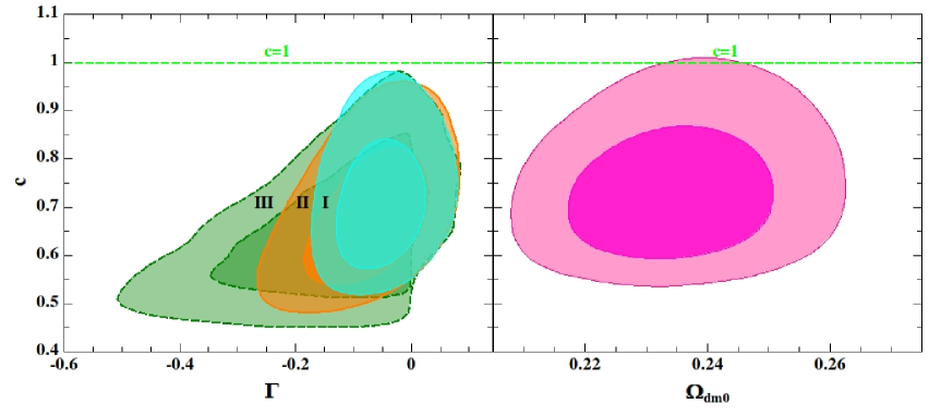
Figure 1: Marginalized probability contours at the $68.3\%$ ($\Delta\chi^{2}=2.3$) and $95.4\%$ ($\Delta\chi^{2}=6.18$) CLs in the $\Gamma$–$c$ (for the three IHDE models) and $\Omega_{dm0}$–$c$ (for the HDE model) planes. The contours for the IHDE1 (cygan, labeled as I), IHDE2 (orange, labeled as II), and IHDE3 (olive, labeled as III) models are plotted in the left panel, and the contours for the HDE model (magnetic) are plotted in the right panel. The green dashed line denotes $c=1$. Clearly, compared with the HDE model, the fitting results of $c$ in the three IHDE models are smaller.

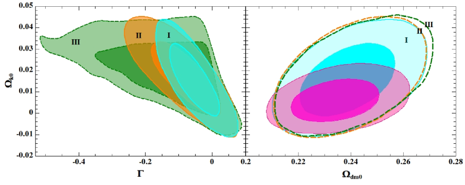
Figure 2: Marginalized probability contours at the $68.3\%$ and $95.4\%$ CLs in the $\Gamma$–$\Omega_{k0}$ (left panel) and $\Omega_{dm0}$–$\Omega_{k0}$ (right panel) planes for the IHDE1 (cygan, labeled as I), IHDE2 (orange, labeled as II), IHDE3 (olive, labeled as III), and the HDE (magnetic) models. The $\Omega_{dm0}$–$\Omega_{k0}$ contours of the three IHDE models are similar to each other, so for the IHDE2 and IHDE3 models, we only plot the 95.4% CL contours.

In the left panel of Fig. 2, we plot the contours of the 68.3% and 95.4% CL for the three IHDE models in the $\Gamma$–$\Omega_{k0}$ plane. The parameter space of the IHDE3 model is much larger than those of the IHDE1 and IHDE2 models, and we can see clear degeneracy between $\Omega_{k0}$ and $\Gamma$, consistent with the result of [19]. The degeneracy amplifies the range of $\Omega_{k0}$ compared with the HDE model without interaction, as is seen in the right panel of Fig. 2, where the contours in the $\Omega_{dm0}$–$\Omega_{k0}$ plane for the three IHDE and the HDE models are all plotted.

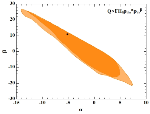
Figure 3: Marginalized probability contours at the $68.3\%$ and $95.4\%$ CLs in the $\alpha$–$\beta$ planes for the IHDE3 model.

We are also interested in the constraints on the parameters $\alpha$ and $\beta$, i.e., the interaction forms allowed by the data. In our analysis, we find the 95.4% CL constraints are

$$\alpha=-5.17^{+13.37}_{-9.59},\ \ \ \beta=10.98^{+18.75}_{-33.42}.$$ (66)

So the allowed regions of $\alpha$ and $\beta$ are very wide. This phenomenon is understandable: the intensity of the interaction term $Q$ is almost decided by $\Gamma$. If $\Gamma$ is small enough, any large values of $\alpha$ and $\beta$ are tolerable. The 68.3% and 95.4% CL contours in the $\alpha$–$\beta$ plane are plotted in Fig. 3, and we can see strong degeneracy between $\alpha$ and $\beta$.

IV.2 Constraints on the interaction term

In this subsection we discuss the constraints on the interaction term in the IHDE models. The fitting results of $\Gamma$ have been listed in the 5-th column of Table 1. We have seen that for all the models we have $\Gamma\leq 0$ at the 68.3% CL. Here we list the 95.4% CL constraints for the three IHDE models,

$$-0.154 \leq \Gamma\leq 0.053\ \ \ \ \rm for\ IHDE1,$$ (67)

$$-0.229 \leq \Gamma\leq 0.059\ \ \ \ \rm for\ IHDE2,$$ (68)

$$-0.509 \leq \Gamma\leq 0.072\ \ \ \ \rm for\ IHDE3.$$ (69)

For the $\Gamma>0$ case, i.e., the direction of the energy flow is from dark energy to dark matter, we find a tight constraint $|\Gamma|\lesssim 0.07$ at the 95.4% CL for all the three IHDE models. For the $\Gamma<0$ case, the allowed value of $\Gamma$ is much larger. At the 95.4% CL, for the IHDE1 and IHDE2 models we have $|\Gamma|\lesssim 0.2$, while for the IHDE3 model we have $|\Gamma|\lesssim 0.5$.

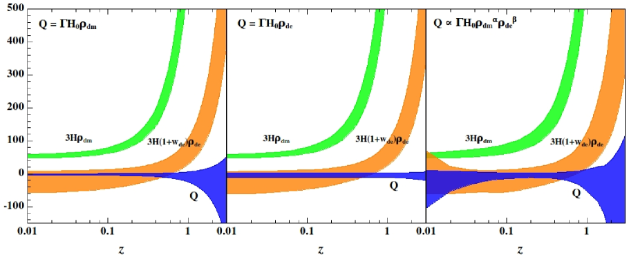
Figure 4: Reconstructed evolutions of $3H\rho_{dm}$, $3H(1+w_{eff})\rho_{de}$ and $Q$ (all divided by $\rho_{c0}$) at the 95.4% CL, for the IHDE1 (left panel), IHDE2 (middle panel) and IHDE3 (right panel) models, respectively.

To see the result more vividly, in Fig. 4 we reconstruct the evolution of $3H\rho_{dm}$, $3H(1+w_{de})\rho_{de}$, and $Q$ at the 95.4% CL for the three IHDE models. As shown in Eqs. (8) and (9), the term $3H\rho_{dm}$ [or, $3H(1+w_{de})\rho_{de}$] characterizes the influence of the cosmic expansion on the energy density of dark matter (or, dark energy), while $Q$ describes the effect of the interaction. As shown in Fig. 4, for all the models $Q$ is much smaller compared with $3H\rho_{dm}$ and $3H(1+w_{de})\rho_{de}$, implying that the influence of interaction on $\dot{\rho}_{dm}$ and $\dot{\rho}_{de}$ is much weaker than the cosmic expansion. It is also interesting to find that the evolution of the interaction terms have different behaviors in the three IHDE models, due to the different expressions of $Q$. In the IHDE1 model with $Q\propto\rho_{dm}$, the absolute value of $Q$ may significantly decrease (along with $\rho_{dm}$) during the evolution, while in the IHDE2 model the absolute value of $Q$ almost maintains no changes during the evolution since $Q\propto\rho_{de}$.

We are interested in the influence of the interaction on the dark matter density, and thus we investigate the quantity $Q/(3H\rho_{dm})$, which describes the ratio between the changes of $\rho_{dm}$ caused by the interaction and by the cosmic expansion. Here we list the constraints on this quantity at $z=0$ at the 95.4% CL,

$$-0.0514\leq\frac{Q}{3H\rho_{dm}}\leq 0.0177\ \ \ \ \rm for\ IHDE1,$$ (70)

$$-0.2097\leq\frac{Q}{3H\rho_{dm}}\leq 0.0625\ \ \ \ \rm for\ IHDE2,$$ (71)

$$-0.4779\leq\frac{Q}{3H\rho_{dm}}\leq 0.0105\ \ \ \ \rm for\ IHDE3.$$ (72)

We see that in the IHDE1 model, the present effect of $Q$ is much smaller than the other two IHDE models. The large value (47.79%) of the lower bound of this ratio in the IHDE3 model indicates that in this model the influence of $Q$ on $\dot{\rho}_{dm}$ can be comparable with that of the cosmic expansion. Figure 4 shows that in the IHDE1 model the present value of $Q$ is much tightly constrained compared with the other two models, and in the IHDE3 model $Q$ could take large negative values when $z\rightarrow 0$.

Also, since we are interested in how much dark matter is produced or annihilated due to the interaction, it is helpful to define another quantity,

$$\Delta\equiv\frac{\rho_{dm}a^{3}\big{|}_{z=0}-\rho_{dm}a^{3}\big{|}_{ini}}{\rho_{dm}a^{3}\big{|}_{ini}}.$$ (73)

Notice that $\rho_{dm}a^{3}$ is the total energy of dark matter in a unit comoving volume. In the absence of interaction, $\rho_{dm}a^{3}$ is conserved, and $\Delta=0$. Here $\rho_{dm}a^{3}\big{|}_{ini}$ is the “initial” value of the total energy of dark matter in a comoving volumn. It can be calculated at the early epoch, e.g., $z>5000$. Thus, $\Delta$ describes the relative change amount of energy in the dark matter component caused by the interaction.

The results for the three IHDE models are as follows:

$$-15.22\% \leq \Delta\leq 8.83\%\ \ \ \ \rm for\ IHDE1,$$ (74)

$$-13.3\% \leq \Delta\leq 5.57\%\ \ \ \ \rm for\ IHDE2,$$ (75)

$$-14.49\% \leq \Delta\leq 6.57\%\ \ \ \ \rm for\ IHDE3.$$ (76)

We find that the results of the three models are not much different from each other. Thus, although the evolution of the interaction term is evidently different, the constraint on the overall effect of the interaction does not change a lot. Roughly, at the 95.4% CL, the increment amount of the energy of dark matter is constrained to be less than 9%, while the decrement amount is constrained to be less than 15%.

IV.3 The fate of the universe

In this subsection we discuss the fate of the universe in the IHDE models. The most important reason for the introduction of the interaction between the dark sectors in the HDE model is to avoid the future big-rip singularity. For the IHDE model with $Q\propto\rho_{dm}^{\alpha}\rho_{dm}^{\beta}$, this issue has been briefly discussed in [17], where it is shown that back reaction effect from quantum corrections cannot prohibit the occurrence of the big rip. Here, we will give a more detailed investigation of the fate of the universe in the IHDE models considered above.

Firstly, we will derive some useful formulas as a preparation of our discussion. Then, we will analyze the dynamical equations to see whether it is possible to avoid the big rip when $c<1$. Finally, based on the constraints of the data, we will numerically solve the equations and reconstruct the evolution of the dark sectors to $z\rightarrow-1$.

IV.3.1 The effective EOS of dark sectors

We can define the effective pressure and effective EOS of dark energy, i.e.,

$$p_{eff,de}=p_{de}+\frac{Q}{3H},\ \ \ w_{eff,de}=w_{de}+\frac{Q}{3H\rho_{de}},$$ (77)

satisfying

$$\dot{\rho}_{de}+3H(\rho_{de}+p_{eff})=0,\ \ \ \dot{\rho}_{de}+3H(1+w_{eff,de})\rho_{de}=0.$$ (78)

From Eq. (13), using $\frac{d}{dt}=-(1+z)H\frac{d}{dz}$ and $\frac{\dot{H}}{H^{2}}=-(1+z)\frac{d\ln H}{dz}=-(1+z)\frac{d\ln E}{dz}$, we derive the equation of state for dark energy,

$$w_{de}=\frac{2(1+z)}{3\Omega_{de}}\frac{d\ln E}{dz}-\frac{1}{\Omega_{de}}-{1\over 3}\frac{\Omega_{r}}{\Omega_{de}}+{1\over 3}\frac{\Omega_{k}}{{\Omega_{de}}}.$$ (79)

Combined with Eq. (24), it follows that

$$w_{de}=-{1\over 3}-{2\over 3}\sqrt{{\Omega_{de}\over c^{2}}+\Omega_{k}}-\frac{\Omega_{I}}{3\Omega_{de}},$$ (80)

which reduces to the familiar formula $w_{de}=-\frac{1}{3}-\frac{2}{3}\frac{\sqrt{\Omega_{de}}}{c}$ when $\Omega_{k}=0$ and $\Omega_{I}=0$. Thus, the effective EOS takes the form

$$w_{eff,de} = w_{de}+\frac{Q}{3H\rho_{de}}$$ (81)

$$= -{1\over 3}-{2\over 3}\sqrt{{\Omega_{de}\over c^{2}}+\Omega_{k}}.$$ (82)

This result is very interesting: $w_{eff,de}$ does not explicitly contain the interaction term. However, we should keep in mind that the evolutions of $\Omega_{de}(z)$ and $E(z)$ are determined by the differential equations (24) and (25) where the interaction $Q$ (or, $\Omega_{I}$) is involved.

It is much easier to derive the effective EOS of dark matter. From Eq. (9), it follows directly that

$$w_{eff,dm} = -\frac{Q}{3H\rho_{dm}}=\frac{\Omega_{I}}{3\Omega_{dm}}$$ (83)

$$= -\frac{1}{3}\Gamma E(z)^{2(\alpha+\beta)-3}\Omega_{dm}^{\alpha-1}\Omega_{de}^{\beta}.$$ (84)

To investigate the fate of the universe, we are also interested in the effective EOS of the total components in the universe, i.e.,

$$w_{eff,tot}=\sum_{i}w_{eff,i}\Omega_{i},$$ (85)

where $i$ represents $de$, $dm$, $b$, $r$ and $k$. In the future epoch, only the dark energy and dark matter components are important.

IV.3.2 Analysis of the dynamical equations in the $z\rightarrow-1$ region

Now we make some general investigations to see whether the big rip can be avoided when $c<1$ in the IHDE models. Equation (82) shows that the effective EOS of HDE is only determined by $\Omega_{de}$ and $c$ (we neglect $\Omega_{k}$ which is less important in the future). In the case of $c<1$, once $\Omega_{de}\rightarrow 1$ there will always be $w_{eff,de}<-1$ and $w_{eff,tot}<-1$, and the fully dominated dark energy will drive the universe to a big rip. Thus, to avoid the big rip, we must evade $\Omega_{de}\rightarrow 1$ in the future. Also, to avoid $\rho_{de}$ from infinitely increasing, we must require $\Gamma>0$, i.e., the direction of energy flow is from dark energy to dark matter.

Here we list the simplified equations of motion in the region $z\rightarrow-1$. Neglecting the radiation, baryon and curvature components, we have

$${1\over E(z)}{dE(z)\over dz}=-{\Omega_{de}\over 1+z}\left({\Omega_{de}-3+\Omega_{I}\over 2\Omega_{de}}+\frac{\sqrt{\Omega_{de}}}{c}\right),$$ (86)

$${d\Omega_{de}\over dz}=-{2\Omega_{de}(1-\Omega_{de})\over 1+z}\left(\frac{\sqrt{\Omega_{de}}}{c}+\frac{1}{2}-{\Omega_{I}\over 2(1-\Omega_{de})}\right).$$ (87)

Notice that unlike the cases of $Q\propto H\rho_{dm}$ or $Q\propto H\rho_{de}$, the two equations are coupled, and thus the situation is much more complicated. However, we find that these equations have a stable point

$$\Omega_{de}=c^{2},\ \ \Omega_{I}=3(1-c^{2}),$$ (88)

which leads to

$$w_{eff,de}=-\frac{1}{3}-\frac{2\sqrt{\Omega_{de}}}{3c}=-1,\ \ \ w_{eff,dm}=-\frac{\Omega_{I}}{3\Omega_{dm}}=-1,\ \ \$$ (89)

and

$$\frac{dE(z)}{dz}=0,\ \ \ \frac{d\Omega_{de}}{dz}=0.$$ (90)

This is exactly a de Sitter solution. See also [37] for a relevant study about the avoidance of big rip in the holographic dark energy model, where the extra dimension effect is considered and the final state of the universe is also a de Sitter solution.

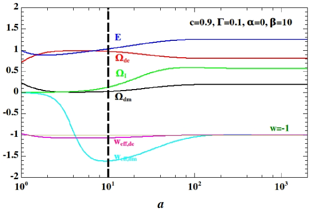
Figure 5: Evolutions of $E$, $\Omega_{de}$, $\Omega_{dm}$, $\Omega_{I}$, $w_{eff,de}$ and $w_{eff,dm}$ along with the scale factor $a$. Here we take typical values of $\Omega_{dm0}=0.24$, $\Omega_{k0}=0$, $h=0.73$, and others are denoted in the panel.

We find that this situation can really happen when $\beta$ is large, and the interaction is strong enough to pull down $\Omega_{de}$ from 1. As an example, in Fig. 5 we demonstrate how the quantities evolve along with the scale factor $a$ in the case of $\beta=10$. A sophisticated discussion on the evolution behaviors of the quantities in the whole range of $a$ would be tedious and unnecessary. Thus, instead, we just focus on the epoch of $a>10$ (the region to the right of the thick dashed line). This would be enough for us to understand how it happens. In this epoch, firstly, $E(z)$ increases due to the dominated dark energy component with $w_{eff,de}<-1$, while the strong interaction pulls $\Omega_{de}$ down from 1. So along with $a$, $\Omega_{de}$ decreases and correspondingly $\Omega_{dm}$ increases. As a result, $w_{eff,de}$ increases from values less than $-1$, while the effective EOS of dark matter, $w_{eff,dm}=\frac{\Omega_{I}}{3\Omega_{dm}}$, which is highly negative due to a small $\Omega_{dm}$, also goes up. When both $w_{de,eff}$ and $w_{dm,eff}$ approach $-1$, the system reaches the stable point, and $E(z)$ stops increasing. The final state of the universe is de Sitter-like.

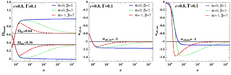
Figure 6: Evolutions of $\Omega_{dm}$ (left panel), $\Omega_{de}$ (left panel), $w_{eff,de}$ (middle panel) and $w_{eff,dm}$ (right panel) along with the scale factor $a$ for three sets of $\alpha$ and $\beta$. The same as Fig. 5, we take values of $\Omega_{dm0}=0.24$, $\Omega_{k0}=0$ and $h=0.73$.

Note that an essential condition that such a procedure can happen is that the interaction is strong enough to pull $\Omega_{de}$ down from 1. Thus, a large $\beta$ is expected. To see the dependence on the values of $\beta$, in Fig. 6 we plot the evolution of $\Omega_{de}$, $\Omega_{dm}$, $w_{eff,de}$ and $w_{eff,dm}$ in large $a$ regions for different values of $\alpha$ and $\beta$. For the case of $\alpha=0$ and $\beta=1$ (the blue line), the interaction is not strong enough to avoid $\Omega_{de}\rightarrow 1$, so the big rip still happens. For the case of $\alpha=0$ and $\beta=3$ (the green dotted line), the interaction is strong enough, and so we see that $\Omega_{de}$ is pulled down from 1, and the system evolves to a stable point when $a>10000$. For the case of $\alpha=-1$ and $\beta=7$ (the red dashed line), the interaction is so strong that the system quickly approaches the stable point at $a<1000$.

In the following, we will numerically solve the equations for the IHDE models in a large $a$ region in the parameter space constrained by the data, and see whether the de Sitter solution can be achieved in these models.

IV.3.3 The IHDE1 and IHDE2 models

In the top panels of Fig. 7 we show the reconstructed evolution of $\Omega_{de}$ along with $z$ for the IHDE1 and IHDE2 models. Clearly, at the 95.4% CL we see $\Omega_{de}\rightarrow 1$ when $z\rightarrow-1$, and we have $w_{eff,de}<-1$ since $c<1$. So these models will not help us to avoid the big rip.

This result is understandable. The fate of the universe in the IHDE model with the interaction term

$$Q=3bH\rho_{de}$$ (91)

was discussed in [9] and it was shown that the condition to prevent the big rip is

$$b\geq c^{-2}-1.$$ (92)

In the IHDE1 and IHDE2 models, analogously, we define the “effective” coupling,

$$b_{eff}\equiv\frac{Q}{3H\rho_{de}},$$ (93)

and we have

$$b_{eff}=\frac{\Gamma\Omega_{dm}}{3E(z)\Omega_{de}},~{}~{}~{}{\rm and}~{}~{}~{}b_{eff}=\frac{\Gamma}{3E(z)}$$ (94)

for the two models, respectively. Note that once $E(z)$ becomes increasing in the future, $b_{eff}$ will be suppressed to zero, so the condition (92) cannot be satisfied.

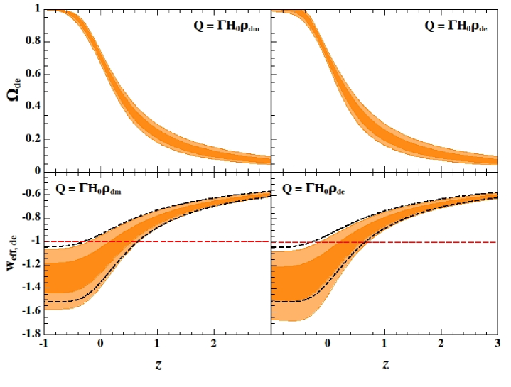
Figure 7: The evolutions of $\Omega_{de}$ (top panels) and $w_{eff,de}$ (bottom panels) along with the redshift $z$ at the 68.3% and 95.4% CLs, for the IHDE1 (left panels) and IHDE2 (right panels) models. The 95.4% CL of HDE model is plotted in dashed lines for a comparison.

The reconstructed $w_{eff,de}(z)$ for the two models are shown in the lower panels of Fig. 7. As a comparison, the 95.4% CL evolution of the HDE model is also plotted (the black dashed line). We see that for these models $w_{eff,de}(z\rightarrow-1)<-1$, and thus the big rip will happen. Also, the values of $w_{eff,de}$ in the IHDE models are more negative than that of the HDE model, since in the two IHDE models $c$ is constrained to be smaller values. Thus, instead of helping us to avoid the big rip, the situation is even worse in these two models.

IV.3.4 The IHDE3 model

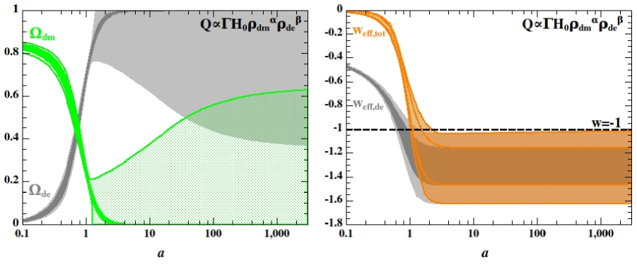
Figure 8: The evolutions of $\Omega_{de}$ (gray, left panel), $\Omega_{dm}$ (green, left panel), $w_{eff,de}$ (gray, right panel) and $w_{eff,tot}$ (orange, right panel) along with the scale factor $a$ for the IHDE3 model. The 68.3% and 95.4% CLs are plotted.

We have seen in Fig. 6 that a large $\beta$ can drive the system to a stable point and avoid the big rip. As shown in Eq. (66) and Fig. 3, in our fitting results we found that large values of $\beta$ are allowed, so we expect that the big rip can be avoided in the IHDE3 model.

In Fig. 8 we plot the evolutions of $\Omega_{de}$ (gray, left panel), $\Omega_{dm}$ (green, left panel), $w_{eff,de}$ (gray, right panel) and $w_{eff,tot}$ (orange, right panel) along with the scale factor $a$ for the IHDE3 model. From the left panel, we see that, at the 68.3% CL $\Omega_{de}\rightarrow 1$ is present in the future due to a negative $\Gamma$ (see Table 1), but the interaction can prevent $\Omega_{de}$ from approaching 1 at the large $a$ region at the 95.4% CL. The right panel shows that the stable point (corresponds to $w_{eff,de}=w_{eff,tot}=-1$) can be accomplished when $a>1000$ at the 95.4% CL. Thus, the IHDE3 model may help to avoid the big rip singularity.

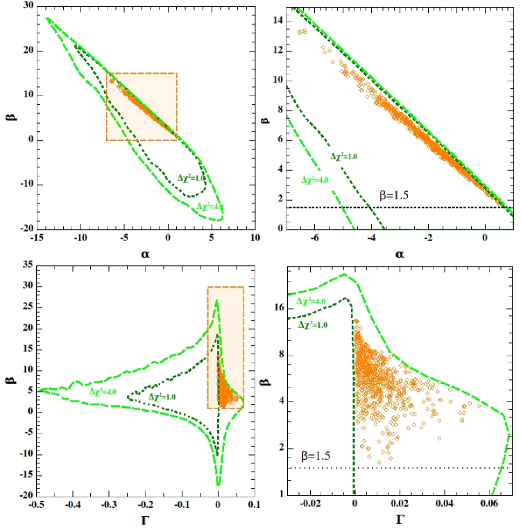
Figure 9: $\Delta\chi^{2}=1$ (olive dotted) and $\Delta\chi^{2}=4$ (green dashed) contours in the $\alpha$–$\beta$ (top panels) and $\Gamma$–$\beta$ (bottom panels) planes. Orange dots are the 709 samples which can achieve a de Sitter solution in the future and thus avoid the big rip. In the left panels the whole contours are plotted, while the right panels, as the zoom in of the dashed orange region of the left panels, show these samples in detail. $\beta=1.5$ is plotted in black dotted lines.

It would be worthy further investigating what kind of samples in our MC analysis may achieve the de Sitter solution. Of $10^{7}$ samples generated for the IHDE3 model there are about 4.7 million samples satisfying $\Delta\chi^{2}<4$. Within them, we find about 18,000 samples satisfying $\Gamma>0$, and finally 709 samples having de Sitter solution in the far future. In Fig. 9, these samples are plotted in the $\alpha$–$\beta$ (top panels) and $\Gamma$–$\beta$ (bottom panels) planes. Clearly, we see that to achieve a de Sitter solution, a large $\beta$ is required (all these samples have $\beta>1.5$). The bottom right panel of the figure shows that, at the 68.3% ($\Delta\chi^{2}<1$) CL, due to a negative $\Gamma$, the big rip cannot be avoided.

V Concluding Remarks

We have investigated the IHDE models with $Q\propto\rho_{dm}^{\alpha}\rho_{de}^{\beta}$. Three IHDE models, including the IHDE1 model with $Q=\Gamma H_{0}\rho_{dm}$, the IHDE2 model with $Q=\Gamma H_{0}\rho_{de}$, and the IHDE3 model with $\alpha$ and $\beta$ running freely, were investigated.

By using the Union2.1+BAO+CMB+$H_{0}$ data, we placed cosmological constraints on these models. We found that a negative $\Gamma$, i.e., energy flow from dark matter to dark energy, is slightly favored by the data, although the HDE model with $\Gamma=0$ still lies in the 95.4% CL region. For all the models, we get $c<1$ at the 95.4% CL. The values of $c$ in the IHDE models are smaller than that in the HDE model.

We showed that the interaction has different properties in the three models. Compared with the cosmic expansion, the effect of interaction on the evolution of $\rho_{dm}$ and $\rho_{de}$ is smaller. We also put a constraint on the total amount of the energy change in the dark matter component. At the 95.4% CL, the increment amount of the dark matter is constrained to be less than 9%, while the decrement amount is constrained to be less than 15%. We found that the constraint basically does not depend on the forms of the interaction term.

Furthermore, we discussed the fate of the universe by investigating the dynamical equations of the IHDE models. We find that the equations may give a de Sitter solution at $z\rightarrow-1$, with the effective equation of state for dark energy and dark matter being $-1$. When confronted with data, we show that this solution cannot be accomplished in the IHDE1 and IHDE2 models. Rather, in these two models since the data favor a smaller $c$, the big rip is even more severe than the HDE model. In the IHDE3 model, we show that such a solution can be achieved for a large $\beta$, and the big rip may be avoided at the 95.4% CL.

Finally, there are still some issues not covered in our paper, i.e., the precise condition for obtaining the de Sitter solution, the coincidence problem, and so on. These issues all deserve further investigations.

- [1] A. G. Riess et al., AJ. 116, 1009 (1998); S. Perlmutter et al., ApJ. 517, 565 (1999).
- [2] D. N. Spergel et al., ApJS 148, 175 (2003); C. L. Bennet et al., ApJS. 148, 1 (2003); D. N. Spergel et al., ApJS 170, 377 (2007); L. Page et al., ApJS 170, 335 (2007); G. Hinshaw et al., ApJS 170, 263 (2007).
- [3] M. Tegmark et al., Phys. Rev. D 69, 103501 (2004); ApJ 606, 702 (2004); Phys. Rev. D 74, 123507 (2006).
- [4] V. Sahni and A. Starobinsky, Int. J. Mod. Phys. D9, 373 (2000); P. J. E. Peebles and B. Ratra, Rev. Mod. Phys. 75, 559 (2003); T. Padmanabhan, Phys. Rept. 380, 235 (2003); E. J. Copeland, M. Sami and S. Tsujikawa, Int. J. Mod. Phys. D 15, 1753 (2006); A. Albrecht et al., astro-ph/0609591; J. Frieman, M. Turner and D. Huterer, Ann. Rev. Astron. Astrophys 46, 385 (2008); S. Tsujikawa, arXiv:1004.1493; V. Sahni and A. Starobinsky, Int. J. Mod. Phys. D15, 2105 (2006); M. Li et al., Commun. Theor. Phys. 56, 525 (2011).
- [5] E. Witten, arXiv:hep-ph/0002297.
- [6] G. ’t Hooft, gr-qc/9310026; L. Susskind, J. Math. Phys. 36, 6377 (1995); J. D. Bekenstein, Phys. Rev. D 7, 2333 (1973); J. D. Bekenstein, Phys. Rev. D 9, 3292 (1974); J. D. Bekenstein, Phys. Rev. D 23, 287 (1981); J. D. Bekenstein, Phys. Rev. D 49, 1912(1994); S. W. Hawking, Commun. Math. Phys. 43, 199 (1975); S. W. Hawking, Phys. Rev. D 13, 191 (1976).
- [7] A. G. Cohen, D. B. Kaplan and A. E. Nelson, Phys. Rev. Lett. 82, 4971 (1999).
- [8] M. Li, Phys. Lett. B 603, 1 (2004).
- [9] M. Li, C. S. Lin and Y. Wang, JCAP 0805, 023 (2008).
- [10] X. Zhang and F. Q. Wu, Phys. Rev. D 76, 023502 (2007); Z. Chang, F. Q. Wu and X. Zhang, Phys. Lett. B 633, 14 (2006); J. Y. Shen, B. Wang, E. Abdalla and R. K. Su, Phys. Lett. B 609, 200 (2005); Z. L. Yi and T. J. Zhang, Mod. Phys. Lett. A 22, 41 (2007); M. Li, X. D. Li, S. Wang and X. Zhang, JCAP 0906, 036 (2009); X. Zhang, Phys. Rev. D 79, 103509 (2009); L. X. Xu et al., Mod. Phys. Lett. A 25, 1441 (2010); Z. P. Huang and Y. L. Wu, arXiv:1202.3517.
- [11] C. J. Hogan, astro-ph/0703775; arXiv:0706.1999; J. W. Lee, J. Lee and H. C. Kim, JCAP 0708, 005 (2007); M. Li et al., Commun. Theor. Phys. 51, 181 (2009); M. Li and Y. Wang, Phys. Lett. B 687, 243 (2010); M. Li, R. X. Miao and Y. Pang, Phys. Lett. B 689, 55 (2010); M. Li, R. X. Miao and Y. Pang, Opt. Express 18, 9026 (2010).
- [12] Q. G. Huang and Y. G. Gong, JCAP 0408, 006 (2004); X. Zhang and F. Q. Wu, Phys. Rev. D 72, 043524 (2005); B. Wang, E. Abdalla and R. K. Su, Phys. Lett. B 611, 21 (2005); S. Nojiri and S. D. Odintsov, Gen. Rel. Grav. 38, 1285 (2006); J. Zhang, X. Zhang and H. Y. Liu, Eur. Phys. J. C 52, 693 (2007); C. J. Feng, Phys. Lett. B 633, 367 (2008); H. Wei and R. G. Cai, Phys. Lett. B 655, 1 (2007); R. G. Cai, Phys. Lett. B 657, 228 (2007); C. Gao, F. Wu, X. Chen and Y. G. Shen, Phys. Rev. D 79, 043511 (2009); C. J. Feng and X. Zhang, Phys. Lett. B 680, 399 (2009); M. Li, X. D. Li and X. Zhang, Sci. China Phys. Mech. Astron. 53, 1631 (2010).
- [13] Q. G. Huang and M. Li, JCAP 0408, 013 (2004).
- [14] Q. G. Huang and M. Li, JCAP 0503, 001 (2005); X. Zhang, Int. J. Mod. Phys. D 14, 1597 (2005); Phys. Lett. B 648, 1 (2007); Phys. Rev. D 74, 103505 (2006); B. Chen, M. Li and Y. Wang, Nucl. Phys. B 774, 256 (2007); J. F. Zhang, X. Zhang and H. Y. Liu, Phys. Lett. B 651, 84 (2007); H. Wei and S. N. Zhang, Phys. Rev. D 76, 063003 (2007); Y. Z. Ma and X. Zhang, Phys. Lett. B 661, 239 (2008); B. Nayak and L. P. Singh, Mod. Phys. Lett. A 24, 1785 (2009); K. Y. Kim, H. W. Lee and Y. S. Myung, Mod. Phys. Lett. A 24, 1267 (2009); Y. G. Gong and T. J. Li, Phys. Lett. B 683, 241 (2010); L. N. Granda, A. Oliveros and W. Cardona, Mod. Phys. Lett. A 25, 1625 (2010); M. J. S. Houndjo and O. F. Piattella, Int. J. Mod. Phys. D21, 1250024 (2012); M. J. S. Houndjo et al., arXiv:1203.6084; Z. P. Huang and Y. L. Wu, arXiv:1202.4228.
- [15] B. Wang, Y. G. Gong and E. Abdalla, Phys. Lett. B 624, 141 (2005); B. Wang, C. Y. Lin and E. Abdalla, Phys. Lett. B 637, 357 (2006).
- [16] H. M. Sadjadi and M. Honardoost, Phys. Lett. B 647, 231 (2007); K. Y. Kim, H. W. Lee and Y. S. Myung, Mod. Phys. Lett. A 22, 2631 (2007); B. Wang, C. Y. Lin, D. Pavon and E. Abdalla, Phys. Lett. B 662, 1 (2008); J. Zhang, X. Zhang and H. Liu, Phys. Lett. B 659, 26 (2008).
- [17] Y. Z. Ma, Y. Gong and X. L. Chen, Eur. Phys. J. C 60, 303 (2009).
- [18] C. Clarkson, M. Cortes and B. A. Bassett, JCAP 0708, 011 (2007).
- [19] M. Li et al., JCAP 0912, 014 (2009).
- [20] C. G. Böhmer, Phys. Rev. D 78, 023505 (2008).
- [21] A. Lewis and S. Bridle, Phys. Rev. D 66, 103511 (2002).
- [22] N. Suzuki et al., arXiv:1105.3470.
- [23] E. Komatsu et al., ApJS. 192, 18 (2011).
- [24] W. J. Percival et al., MNRAS 401, 2148 (2010).
- [25] D. H. Jones et al., MNRAS 399, 683 (2009); F. Beutler, et al., arXiv:1106.3366, MNRAS accepted.
- [26] M. Drinkwater et al., MNRAS 401, 1429 (2010); C. Blake et al., arXiv:1108.2635, MNRAS accepted.
- [27] A. G. Riess et al., ApJ. 730, 119 (2011).
- [28] L. Perivolaropoulos, Phys. Rev. D 71, 063503 (2005); S. Nesseris and L. Perivolaropoulos, Phys. Rev. D 72, 123519 (2005); S. Nesseris and L. Perivolaropoulos, JCAP. 0702, 025 (2007).
- [29] http://supernova.lbl.gov/Union/
- [30] W. Hu and N. Sugiyama, ApJ 471, 542 (1996).
- [31] J. R. Bond, G. Efstathiou and M. Tegmark, MNRAS 291, L33 (1997).
- [32] R. Lazkoz, R. Maartens and E. Majerotto, Phys. Rev. D 74, 083510 (2006); O. Elgaroy and T. Multamaki, astro-ph/0702343; M. Li, X. D. Li and S. Wang, arXiv:0910.0717; M. X. Lan, M. Li, X. D. Li and S. Wang, Phys. Rev. D 82, 023516 (2010); S. Wang, X. D. Li, and M. Li, Phys. Rev. D 82, 103006 (2010); H. Wei, JCAP 1008, 020 (2010); Y. H. Li, J. Z. Ma, J. L. Cui, Z. Wang and X. Zhang, Sci. China G 54, 1367 (2011); T. F. Fu, J. F. Zhang, J. Q. Chen and X. Zhang, Eur. Phys. J. C 72, 1932 (2012).
- [33] D. J. Eisenstein et al., ApJ 633, 560 (2005).
- [34] D. J. Eisenstein and W. Hu, ApJ. 496, 605 (1998).
- [35] W. L. Freedman and B. F. Madore, arXiv:1004.1856.
- [36] W. Hu, ASP Conf. Ser. 339, 215 (2005).
- [37] X. Zhang, Phys. Lett. B 683, 81 (2010).